Abstract
As essential environmental parameters in the greenhouse, appropriate light and CO2 will improve agricultural productivity and quality. Although many related studies have been carried out on the intelligent regulation of these environmental factors, the regulation of light and CO2 is usually controlled separately, and energy consumption is rarely considered. This paper proposed a coordinated control strategy for greenhouse light and CO2 based on the multi-objective optimization model. Firstly, the experiments on the net photosynthetic rate of blueberry under different temperatures, photon flux density, and CO2 concentration nesting were carried out to establish a blueberry net photosynthetic rate prediction model based on Support Vector Regression (SVR). Secondly, a model for calculating the energy cost of both light and CO2 was constructed. Thirdly, taking the maximum net photosynthetic rate and the minimum energy cost as the objective functions, the Non-dominated Sorting Genetic Algorithm (NSGA-II) was leveraged to obtain the Pareto optimal solutions of the target regulation values of light and CO2 concentration in different temperature ranges. Then, the optimal values were selected based on two different strategies. Finally, the multi-objective optimal control strategy proposed in this paper was compared with both the classical threshold control strategy and the Gaussian curvature maximization control strategy. The results indicated that the strategy which prioritized energy saving could reduce the energy cost by about 22.33% and 19.08%, respectively, under the premise that the net photosynthetic rate was consistent. Meanwhile, the strategy that prioritized production efficiency could increase the net photosynthetic rate by about 8.40% and 4.42%, respectively, with the same energy cost. In conclusion, the proposed multi-objective optimization control can improve the greenhouse climate control performance and reduce cost compared with other mentioned strategies.
1. Introduction
The optimum control of a greenhouse climate is one of the most important factors for the rapid development of the agriculture industry. Through the actuators to adjust the light, CO2, temperature, and other climate variables to maintain the ideal environment, greenhouse crops are set in the best growth conditions. Therefore, cultivation inside the greenhouse results in better quality and greater yield [,,]. Among the mentioned factors, light plays a key role in establishing and regulating the internal biological clock of plants and is one of the important parameters affecting the formation of crop growth morphology and the accumulation of functional chemicals, thus determining the productivity of greenhouse crops [,]. The regulation of light intensity is also linked to the physiological processes of greenhouse crops, including stomatal scheduling [] and leaf development [], etc. In terms of the regulation of the light environment, existing studies have adopted a dynamic threshold light supplement strategy based on the physiological characteristics of crops []. Some researchers have also used genetic algorithms to dynamically obtain light saturation points to build an optimal regulation model of photosynthesis [].
CO2 works as the direct reactant of photosynthesis in a greenhouse environment []. Thus, the rise of CO2 will directly affect many physiological characteristics of crops, such as transpiration rate and net carbon exchange rate []. In terms of CO2 control, previous studies have focused on threshold control with fixed values []. These control methods are not accurate enough, since they ignore the changes during the control process, which will lead to a low utilization rate of CO2 and energy waste. To achieve efficient regulation of CO2, some researchers have established CO2 response curves in different light and temperature intervals and taken the points of maximum curvature as target values [,].
Although many related studies have been carried out on intelligent regulation from different perspectives, most of these are single variable control, which lacks the synergistic control of phosgene in this dynamic environment [,]. After all, due to the dependency between each state of the system, the difficulty of effective control will increase [,]. However, the interaction effects of microclimate factors are supposed to be considered in the regulation process []. With the development of computer performance and machine learning methods, many advanced approaches have been used in multi-factor coordinated control of greenhouse environment, and system optimization, particularly in industrial applications, has been significantly considered by many researchers [,]. The classical control experience combined with effective algorithms can finally realize the synchronous control of multiple system states of microclimate in a modern greenhouse [,,]. In these studies, however, the models lack consideration of plants condition or energy consumption, which may lead to a worse quality of crops or higher control cost [,,].
Thus, to overcome the aforementioned obstructions, this study explored a control strategy of light and CO2 supplements, considering both energy cost and net photosynthetic rate. Specifically, the support vector regression method was utilized to construct a photosynthetic rate prediction model based on temperature, light intensity, and CO2 concentration. At the same time, the energy cost model of greenhouse light and CO2 supplement was constructed. Based on the models mentioned above, the maximum net photosynthetic rate and the minimum energy cost were taken as the objectives. The multi-objective optimization of the CO2 concentration and light intensity regulation values was conducted to obtain economically optimal results. In our previous work, we have proposed a greenhouse environment multi-factor coordinated control algorithm [,,], which effectively solves the coordination and energy-saving control of temperature and humidity, and effectively reduces the cost of temperature and humidity control such as ventilation and heating. However, in that algorithm, the control target values of light and CO2 are obtained based on agricultural experience without considering the optimization of benefits such as energy conservation. Therefore, we will study the optimization of the coordinated control strategy of greenhouse light and CO2 in this paper.
2. Materials and Methods
2.1. Data Collection and Processing
The experimental site was located in the southeast of Kunshan City, Jiangsu Province, China ( N and E), where the sunrise was roughly 5:00–5:50 and sunset was roughly 18:30–19:00. The experimental greenhouse was a Venlo-type glass greenhouse, which had small roof skylights. The framework was made of aluminum alloy material. Both the covering and side wall were made of single-layer tempered glass. Thus, it had the characteristics of high light transmittance, long service life, and large operating space. The span of the greenhouse was about 17.5 m, the ridge height was about 7.2 m, the land area was about 297.5 , and the total volume was about 1918.875 . The exterior and interior of the experimental greenhouse were shown in Figure 1. The southern highbush blueberry named “Emerald”, which was relatively resistant to moisture and heat, was selected as the experiment subject and planted in the culture tank with sufficient water and fertilizer. The pH of the nutrient soil was controlled between 4.5 and 5.5. The temperature requirements of blueberries in different phenological stages were not the same. According to the different characteristics of blueberry phenology, it can be roughly divided into dormant period, budding period, flowering period, fruit period, and flower bud differentiation period. Our study was mainly conducted in spring and summer, when blueberries were in the flower and fruit growth period. Based on planting experience, the target temperatures are 25–35 °C in the daytime and 15–22 °C in the night. During this experiment, the daily crop maintenance was carried out routinely without any additional operations.
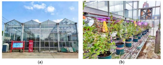
Figure 1.
The exterior (a) and interior (b) of the experimental greenhouse.
The data collection started in March and ended in August 2021. During the period, blueberry plants with small growth differences were selected. For each plant, the third functional leaf with healthy growth status was designated as the test sample. Considering the impact of the crop “siesta phenomenon” on the accuracy, the measuring process was divided into two periods: 8:00–11:30 and 14:30–17:30. The measuring device was the Li-6400XT portable photosynthesis measurement system. The temperature gradients were set to 20, 24, 28, 32, 36, and 40 °C, respectively. The photon flux density gradients were set to 0, 50, 100, 300, 500, 700, 900, 1200, 1500, 1800, 2100, and 2400 , respectively. The carbon dioxide concentration gradients were set to 0, 50, 100, 300, 400, 500, 700, 1000, 1300, 1600, 1900, and 2200 , respectively. In measurement, there might be some operation errors such as the improper position of blade clamping, which made the measured value deviate from the actual net photosynthetic rate of crops, resulting in invalid data. The corresponding technique was to eliminate the invalid data, re-measuring the leaf under the current environment until the three net photosynthetic rate measurements of blueberries were all valid. Next, the average of this dataset was recorded for subsequent operations. According to the above description, 1152 sets of blueberry net photosynthetic rate datasets were obtained, with temperature, photon flux density, and carbon dioxide concentration as inputs.
2.2. Net Photosynthetic Rate Prediction Model
Crop yield is one of the most important indicators to measure the efficiency of greenhouse production, but the complexity of crop physiological characteristics makes it difficult to predict the yield during growth. Photosynthetic rate, as the main indicator to measure the photosynthetic capacity of crops, has a significant nonlinear relationship with photon flux density, temperature, and CO2 concentration []. The support vector machine is mathematically valid and generalizing, which can be used for the construction of nonlinear models []. Support vector regression is a generalization of a support vector machine []. Different from the Empirical Risk Minimization (ERM) principle used in conventional neural networks, support vector regression adopted the Structural Risk Minimization (SRM) principle. By minimizing the upper bound of the generalization error, the support vector regression has a stronger generalization capability []. The basic idea of a support vector regression is to map data to a high-dimensional feature space through nonlinear mapping. Different from classical regression models, the model output is not required to be the same as the real output , but introduces a tolerable deviation ε []. In this study, a prediction model of blueberry net photosynthetic rate was constructed based on support vector regression. Temperature, CO2 concentration, and photon flux density, which were significantly related to photosynthetic rate, were selected as input , and the net photosynthetic rate was selected as output . The model building process is shown in Figure 2.
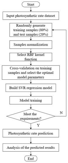
Figure 2.
Flow chart of the photosynthetic rate prediction model.
In this study, Radial Basis Function (RBF) was introduced into the modeling process, and thus the regression function was obtained as follows []:
where
In the functions above, stood for the number of support vectors, represented support vectors, stood for bias, was the dual optimal solution, was the radial basis kernel function, and was the width.
In the 1152 sets of data containing temperature, CO2 concentration, light intensity, and corresponding net photosynthetic rate, 922 sets of data were randomly selected for training (accounting for 80% of the total), and the remaining 230 sets of data were used as a test set to check the prediction accuracy (accounting for 20% of the total). The “fitrsvm” function in MATLAB was called to get the regression model. The kernel function was set to ‘gaussian’ or ‘rbf’ and ‘Standardize’ as ‘True’ to normalize the predictor data. Besides, other parameters were set as the default values.
2.3. Cost Function of Energy Consumption in CO2 Supplement
The increase of CO2 concentration in the greenhouse mainly depended on artificial replenishment. Beyond that, the organic decomposition of microorganisms in soil and the respiration of crops would also increase CO2 concentration. The depletion of CO2 mainly depended on the absorption of photosynthesis by crops. In addition to the above factors, air exchange happened through windows and wall cracks, which would change the indoor CO2 concentration. The dynamic entry and exit paths of CO2 inside the greenhouse are shown in Figure 3.
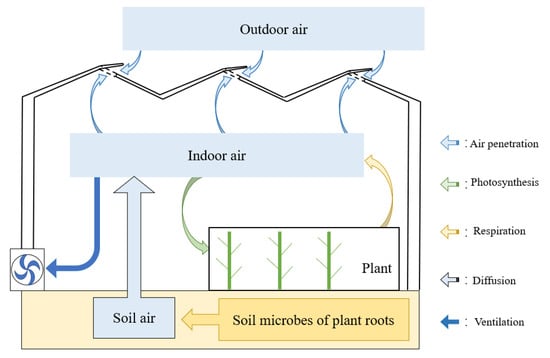
Figure 3.
Dynamic entry and exit paths of CO2 in the greenhouse.
Based on the above analysis, the dynamic equilibrium of CO2 concentration in the greenhouse could be expressed as follows:
where V represented the greenhouse volume, was the change value of indoor CO2 concentration, stood for the CO2 released by soil microbial decomposition, represented the CO2 of external application, represented the CO2 of crop photosynthetic consumption, represented the CO2 produced by crop respiration, stood for the CO2 exchanged between the skylight and the side window, and represented the amount of change in the CO2 caused by air exchange in the crevices of building materials.
The above dynamic equilibrium of CO2 concentration in the greenhouse worked as theoretical analysis, and the specific parameters could be adjusted according to the actual operation of the greenhouse. In the Kunshan Greenhouse, where this experiment was conducted, blueberry plants were cultivated in plastic pots filled with nutrient soil, and the walkways were masonry ground with covering cloth. Therefore, CO2 released through ground soil and cultivation substrates was relatively limited and negligible, so was set to zero. Experimental crops were generally in the growing stage, which required artificial CO2 supply to promote the accumulation of photosynthetic products, and it was necessary to maintain a higher indoor concentration of CO2 to promote crop fruit accumulation. Therefore, was set to zero in Formula (4). In addition, considering the presence of photosynthesis and respiration of crops during the day, the net CO2 absorbed by photosynthesis of crops could be simplified as follows:
The net CO2 consumed by crop photosynthesis was significantly correlated with the total leaf area and the net photosynthetic rate intensity per unit area, which could be expressed as follows:
where represented the total net photosynthesis of crops per unit time, was the planted area of the greenhouse, represented the leaf area index, and was the net photosynthetic rate per unit area. The design architecture and construction materials of the greenhouse might also lead to indoor and outdoor air exchange in wall gaps, and the resulting CO2 change could be expressed as follows:
where represented the amount of CO2 change resulting from air exchange in wall gaps per unit time, was the influencing factor of gap ventilation, represented indoor CO2 concentration, and was outdoor CO2 concentration. The value of air exchange in wall cracks varied greatly due to the different conditions of the greenhouse. Moreover, since the parameter values of the building materials were difficult to determine and may even change with different climate factors, relevant studies mostly refer to the empirical design value and then adjust it according to the actual situation [].
Considering the above factors, the simplified indoor CO2 inflow and outbalance model for the potted blueberry glass greenhouse could be obtained as follows:
convert the above equation to a transient dynamic change model:
where represented the real-time supply of CO2 per unit time. In conclusion, the CO2 consumption model of potted blueberry photosynthesis on the masonry floor was obtained as follows:
where stood for CO2 consumption per unit time, represented the target value of CO2 regulation, represented the initial value of CO2 regulation, and [, ] stood for a unit regulation period interval.
2.4. Cost Function of Energy Consumption in Light Supplement
The cost of light replenishment was also a large term in greenhouse cost, and the specific calculation formula could be described as follows []:
where was the energy consumption of supplemental light in the greenhouse, represented the influence factor of light energy conversion, was the greenhouse light regulation target value, and represented the initial value of greenhouse light regulation. Considering the physiological characteristics of blueberry during the growth, the periods of supplementary light in this study were approximately 6:30–8:00, 16:00–19:00. If the weather was cloudy or rainy outside, extra light would be added to ensure the blueberry’s light demand.
2.5. Energy Cost Model of Light and CO2
Based on the above analysis and the market price factors, the total energy cost model of supplemental light and CO2 in spring and summer for the experimental blueberry greenhouse can be expressed as:
where and were the energy cost coefficients of compensating light and CO2, respectively. The CO2 supplement in this experiment depended on the gas cylinder with a diameter of 0.2 m and a height of 1.2 m, which could be recycled for multiple uses and was not considered a consumable material. Therefore, it was only necessary to calculate the price of CO2 according to the market, and the energy cost coefficient was calculated as 0.345. The replenishment light was mainly based on indoor lights, which required a large amount of power energy [,]. According to the market, the economic loss coefficient of replenishment light was 0.6 × 10⁻³.
2.6. Multi-Objective Optimization Model of Light and CO2 Coordination
The increase in the net photosynthetic rate required sufficient light and CO2 supply, which would lead to an increase in energy consumption. On the contrary, the pursuit of energy conservation required a reduction in energy consumption, which affected the photosynthesis of crops. Reasonable greenhouse regulation required coordination and compromise between net photosynthetic rate and economic loss to achieve the optimal overall goal as far as possible. Therefore, this study adopted a multi-objective optimization method to get the Pareto optimization solution.
2.6.1. Multi-Objective Optimization Function Model
Since the net photosynthetic rate conflicted with the economic loss and was of different dimensions, multi-objective optimization was selected to obtain the multi-objective regulation value of the greenhouse environment. The maximum net photosynthetic rate and the minimum economic loss were set as two sub-objectives and combined with the above mechanism model, and the multi-objective function as shown below was constructed:
where in the above model was a two-dimensional decision variable to be optimized:
where represented the target regulation value of indoor CO2, and was the target regulation value of indoor illumination. According to the climatic conditions and blueberry growth habits of the test greenhouse, the constraint conditions of CO2 concentration and light in the optimization process were set as follows:
where was the multi-objective function to be optimized, was the lower limit of the CO2 concentration, and was the upper limit of the CO2 concentration. The represented the initial light intensity, and the was the upper limit of the light intensity.
2.6.2. Multi-Objective Optimization Algorithm
The core of a multi-objective optimization algorithm lies in the coordination and compromise of each objective function so that it can achieve relatively better results as far as possible. In this work, NSGA-II (Non-dominated Sorting Genetic Algorithms-II) proposed by Deb was selected to solve the multi-objective problem. According to this algorithm, the fast non-dominated sorting strategy, elite strategy, and density value estimation strategy were introduced to improve the search performance []. Relevant theories and advantages of this algorithm could be referred to in the literature [], and specific steps are shown in Figure 4.
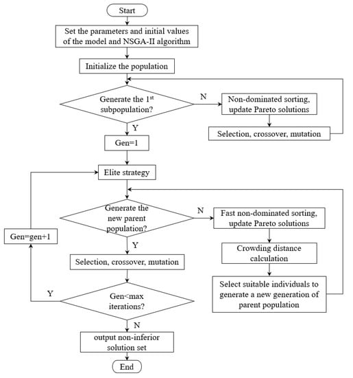
Figure 4.
Steps of NSGA-II.
3. Results and Discussions
All experiments were implemented on the same system with an Intel® CoreTM i5-11300H @ 3.10 GHz CPU and a 16.00 GB RAM. The software required for the simulation test was MATLABTM with version R2021a.
3.1. Verification and Analysis of the SVR Model
According to the established SVR model, the predicted output of net photosynthetic rate under different light intensities and CO2 concentration was shown in Figure 5. Since the overall trend at different temperatures was very consistent, the relationship diagram under 28 °C was selected as an example. It could be seen that the influence of both photon flux density and CO2 on the net photosynthetic rate of crops was consistent. The increase in light intensity and CO2 concentration would increase the photosynthetic rate in the beginning, but the photosynthetic rate tended to be stable near the light saturation point. At this time, the addition of light and CO2 would inhibit the photosynthetic rate.
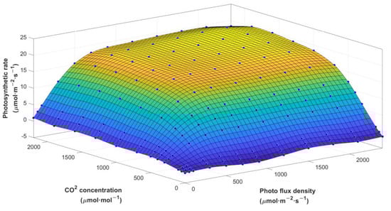
Figure 5.
Change of photosynthetic rate values under photon flux density and CO2 concentration.
To verify the accuracy of the prediction model of blueberry net photosynthetic rate based on the support vector regression algorithm, the deviation between the measured value and the predicted value of the model was used as the benchmark for model evaluation. The validation set consists of two parts. As mentioned before, 20% of the total dataset was selected as the validation set. To further verify the accuracy and generalization ability of the blueberry net photosynthetic rate prediction model, another 100 sets of greenhouse climate data measured from 8:00–11:30 and 14:00–18:00 in July and August were also added. The data types of each group in the additional validation set were the same as those in the original dataset, including temperature, light intensity, CO2 concentration, and corresponding net photosynthetic rate of crops. To measure the error rate of the prediction, we used several statistical metrics [,]: Mean Absolute Error (MAE), Mean Relative Error (MRE), Root Mean Square Error (RMSE), and Coefficient of Determination (R2), which were calculated as follows:
The evaluation indexes of the predictive effect of the net photosynthetic rate model under the two validation sets are shown in Table 1 (ran five times continuously to reduce the impact of randomness, and the worst result was selected).

Table 1.
Evaluation index of the net photosynthetic rate prediction model.
In the table above, the values of MAE, MRE, and RMSE for two validation sets were all within certain accuracy ranges. In Figure 6, the green triangle represented the relationship between the predicted photosynthetic rate and the measured value in the divided 20% test set, and the blue line represented the fitting line. The blue circle represented the relationship between the predicted and measured photosynthetic rates in the additional test set, and the blue line represented the fitting line. Due to the overlap of these two fit lines, we bolded the fitting line of the additional test set to ensure that it could be clearly seen. As the figure showed, the points in the two datasets were fairly close to the fitting line, and the Coefficient of Determination (R2) reached more than 0.99, indicating that there was a high linear correlation between the measured values and the predicted values.
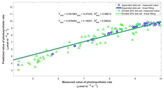
Figure 6.
Correlation of measured and simulated values in appended dataset (blue) and divided 20% test set (green).
3.2. Verification and Analysis of Multi-Objective Optimization
Based on the net photosynthetic rate prediction model and the energy cost model, a set of optimal solutions was obtained, namely, the Pareto Frontier. The initial population number of the NSGA-II optimization process was set as 100 and the maximum iteration number was 200. We selected the initial value = [400, 200], the minimum value = [0, 0], and the maximum value = [2200, 2400]. The solving process was run 10 times at each temperature, and the Pareto Frontier obtained after a random run is shown in Figure 7. Note that the x-axis represented the negative of photosynthetic rate. Since the general trends of curves at different temperatures were similar in shape, the Pareto Frontier at 28 °C was selected here as an example. It was obvious that the rise in photosynthetic rate would increase energy cost, and vice versa, which characterized the contradiction between multiple objectives.
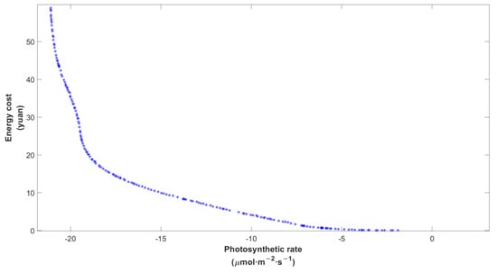
Figure 7.
Pareto Frontier after multi-objective optimization at 28 °C. Each blue individual dot represented an optimal solution in the current state, and the blue curve formed was the Pareto Frontier of this operation.
3.3. Comparison and Analysis
To further verify the regulation effect of this multi-objective optimization model, six testing sets were divided by different temperatures at 20 °C, 24 °C, 28 °C, 32 °C, 36 °C, and 40 °C. The CO2 concentration and light intensity of the experimental greenhouse were measured from 08:00 to 18:00 in two days in May 2021, and their mean values were taken as the initial control values. Thus, the initial value of CO2 concentration was 438 , and the initial value of light was 330 . After obtaining the optimal solution by multi-objective optimization, the appropriate light and CO2 target values were selected based on two regulatory strategies.
According to the non-dominated solution selected, the values of energy cost and photosynthetic rate of blueberry were compared with those obtained from the classical threshold regulation and the Gaussian curvature maximization regulation, respectively. In this study, the threshold control strategy of the greenhouse was set as follows: when the indoor CO2 concentration was less than 1000 , we supplied CO2 to the greenhouse until the setting value was reached. Similarly, when the light intensity was less than 600 , we added extra light to the blueberries until the setting value was reached. As for the Gaussian curvature function, it was a control strategy based on gaussian curvature maximization: according to the Gaussian curvature function of the blueberry photosynthetic rate mechanism model, the fitness function was constructed. Next, Particle Swarm Optimization [] was used to calculate the light intensity and CO2 concentration corresponding to the maximum Gaussian curvature. Finally, a comprehensive regulation strategy of light and CO2 under different temperatures was established based on polynomial fitting. Compared with the maximum net photosynthetic rate saturation point regulation, the regulation strategy based on Gaussian curvature maximization was been proved to effectively improve greenhouse benefits. Further details about Gaussian curvature maximization modulation can be found in the literature [].
3.3.1. Energy Cost Strategy
The goal of modern facility agriculture is not only to improve the yield and quality of agricultural products but also to reduce energy cost in the production process. To be eco-friendly, the selection of energy cost strategy was based on the following principles: when compared with threshold regulation strategy, since we knew the initial values of the environment and the target values of regulation (CO2: 438–1000 , Light: 330–600 ), it was not hard to calculate the photosynthetic rate and total cost. For example, when the temperature was 32 °C (the fourth row in Table 2), we could calculate that the photosynthetic rate was 15.54 and the cost was 9.8799 yuan. To compare the cost of each strategy, we should maintain other conditions in the same. Therefore, we would look for the point in Pareto Frontier which had the closest photosynthetic rate to that in threshold regulation. That is to say, we would find the solution whose photosynthetic rate value was closest to 15.54 , and select the corresponding decision variable values as the target values of light and CO2 regulation. The closest net photosynthetic rate value we found in the solution set was 15.56 , and the corresponding light and CO2 regulation values obtained were 453 and 1700 . Finally, the energy cost to this point was obtained and compared with the energy cost generated by threshold regulation. This selection strategy was repeated in each temperature segment, and the selection process was applied to Gaussian curvature maximization regulation as well. According to the above selection method, the comparison results of the two strategies obtained by simulation are shown in Table 2 and Table 3, respectively.
Table 2.
Comparison of threshold regulation strategy and energy cost strategy.
Table 3.
Comparison of Gaussian curvature maximization modulation and energy cost strategy.
Under the precondition of maintaining the consistent net photosynthesis rate of crops, the results showed that the use of the energy cost strategy could reduce the energy consumption by about 22.33% and 19.08%, respectively, compared with the classical threshold regulation strategy and the gaussian curvature maximization control strategy. Therefore, the energy cost strategy was able to effectively reduce the energy consumption of light and CO2 to achieve the goal of energy saving.
3.3.2. Photosynthesis Improvement Strategy
When the economic cost before the optimization is within the acceptable range, the greenhouse manager hopes to improve the net photosynthetic rate by optimizing the setting values of both indoor carbon dioxide and light regulation. This photosynthesis improvement strategy was very similar to the energy cost strategy mentioned in Section 3.3.1. The main difference was that, after calculating the photosynthetic rate and cost of the threshold regulation strategy, this time we did not seek for the solution with a similar photosynthetic rate, but with a similar cost. Next, we took the decision variable values of this solution as the target values of light and CO2, and compared the photosynthetic rate values under these two regulation strategies. This selection strategy was repeated in each temperature segment, and the selection process was applied to Gaussian curvature maximization regulation as well. The comparison results obtained by simulation are shown in Table 4 and Table 5, respectively.
Table 4.
Comparison of threshold regulation strategy and photosynthesis improvement strategy.
Table 5.
Comparison of Gaussian curvature maximization modulation and photosynthesis improvement strategy.
The results demonstrated that without additional energy cost, the photosynthesis improvement strategy could increase the net photosynthetic rate of blueberries by about 8.40% on average compared with the classical threshold control strategy, and by about 4.42% compared with the Gaussian curvature maximization control strategy. The experimental results proved that the optimization strategy could achieve reasonable regulation of light and CO2 to effectively improve the photosynthetic rate, thereby ultimately promoting product accumulation.
4. Conclusions
This article surveyed the state of the art of light and CO2 control in the greenhouse and presented a multi-objective optimization control strategy. By adopting the SVR approach on collected data, a prediction model of blueberry net photosynthetic rate was constructed, with light intensity, CO2 concentration, and temperature as inputs. The values of evaluation indicators were all within the ideal accuracy range, and the regression coefficients of the two validation sets were above 0.99, which proved that the net photosynthetic rate of blueberries could be predicted precisely. Since the net photosynthetic rate and energy cost functions were different dimensions and inherently conflicting, a NSGA-II multi-objective optimization algorithm was implemented to optimize the target value of the phosgene regulation, and the Pareto optimal solutions in different temperature intervals were obtained. Finally, based on different selection strategies, the regulation results obtained by multi-objective optimization were compared with the classic threshold regulation strategy and the gaussian curvature maximization control strategy in different temperature intervals. On the one hand, the energy cost strategy could save about 22.33% and 19.08%, respectively, under the premise of maintaining the same photosynthetic rate. On the other hand, the photosynthetic improvement strategy could increase the net photosynthetic rate by about 8.40% and 4.42% on average under the premise of maintaining similar energy consumption. Therefore, it was proven that the coordinated control strategy proposed in this paper has a better control efficiency compared to both the classic threshold regulation strategy and the gaussian curvature maximization control strategy. Moreover, this study adopted the multi-objective optimization algorithm, and the result of coordinated optimization is a series of (multiple groups) control target values of light and CO2. Therefore, a significant advantage is that greenhouse managers can choose a set of optimal control target values of light and CO2 according to market changes: if the market price of energy is high, managers can select control target values of light and CO2 according to the “energy cost strategy” so as to reduce energy consumption; if the market price of energy is low, managers can select control target values of light and CO2 according to the “photosynthesis improvement strategy” so as to pursue a higher photosynthetic rate of crops and achieve higher yield. This decision-making method provides a theoretical reference for the comprehensive regulation of light and CO2 in the greenhouse based on different targets. In future work, the experimental validation of the proposed control strategy will be further investigated.
Author Contributions
Conceptualization, X.W.; methodology, X.W.; software, X.W.; validation, X.W. and L.X.; formal analysis, X.W. and L.X.; investigation, X.W.; resources, X.W. and L.X.; data curation, X.W.; writing—original draft preparation, X.W.; writing—review and editing, L.X.; visualization, X.W.; supervision, L.X. and R.W.; project administration, L.X. and R.W.; funding acquisition, L.X. All authors have read and agreed to the published version of the manuscript.
Funding
This work was supported in part by the National Natural Science Foundation of China under Grant 61973337; and in part by Shanghai Municipal Science and Technology Commission Innovation Action Plan under Grant 17391900900.
Data Availability Statement
For source code, interested user is recommended to send a request to the authors (xulihong@tongji.edu.cn).
Acknowledgments
This work was supported in part by the National Natural Science Foundation of China under Grant 61973337; and in part by Shanghai Municipal Science and Technology Commission Innovation Action Plan under Grant 17391900900. The authors would also like to express great appreciation to Huihui Liu for his valuable and constructive suggestions.
Conflicts of Interest
The authors declare no conflict of interest.
References
- Von Zabeltitz, C. Integrated Greenhouse Systems for Mild Climates: Climate Conditions, Design, Construction, Maintenance, Climate Control; Springer Science & Business Media: Berlin/Heidelberg, Germany, 2010. [Google Scholar]
- Mahdavian, M.; Sudeng, S.; Wattanapongsakorn, N. Multi-objective optimization and decision making for greenhouse climate control system. In Proceedings of the 2016 International Conference on Information Science and Security (ICISS), Pattaya, Thailand, 19–22 December 2016; pp. 1–5. [Google Scholar]
- Rodríguez, F.; Berenguel, M.; Guzmán, J.L.; Ramírez-Arias, A. Climate and irrigation control. In Modeling and Control of GREENHOUSE Crop Growth; Springer: Cham, Switzerland, 2015; pp. 99–196. [Google Scholar]
- De Andrade, M.V.S.; de Castro, R.D.; da Silva Cunha, D.; Neto, V.G.; Carosio, M.G.A.; Ferreira, A.G.; de Souza-Neta, L.C.; Fernandez, L.G.; Ribeiro, P.R. Stevia rebaudiana (Bert.) Bertoni cultivated under different photoperiod conditions: Improving physiological and biochemical traits for industrial applications. Ind. Crops Prod. 2021, 168, 113595. [Google Scholar] [CrossRef]
- Jishi, T.; Matsuda, R.; Fujiwara, K. Effects of photosynthetic photon flux density, frequency, duty ratio, and their interactions on net photosynthetic rate of cos lettuce leaves under pulsed light: Explanation based on photosynthetic-intermediate pool dynamics. Photosynth. Res. 2018, 136, 371–378. [Google Scholar] [CrossRef] [PubMed]
- O’Carrigan, A.; Hinde, E.; Lu, N.; Xu, X.-Q.; Duan, H.; Huang, G.; Mak, M.; Bellotti, B.; Chen, Z.-H. Effects of light irradiance on stomatal regulation and growth of tomato. Environ. Exp. Bot. 2014, 98, 65–73. [Google Scholar] [CrossRef]
- Evans, J.; Poorter, H. Photosynthetic acclimation of plants to growth irradiance: The relative importance of specific leaf area and nitrogen partitioning in maximizing carbon gain. Plant Cell Environ. 2001, 24, 755–767. [Google Scholar] [CrossRef]
- Xu, L.; Wei, R.; Xu, L. Optimal greenhouse lighting scheduling using canopy light distribution model: A simulation study on tomatoes. Light. Res. Technol. 2020, 52, 233–246. [Google Scholar] [CrossRef]
- Hu, J.; He, D.; Ren, J.; Liu, X.; Liang, Y.; Dai, J.; Zhang, H. Optimal regulation model of tomato seedlings’ photosynthesis based on genetic algorithm. Trans. Chin. Soc. Agric. Eng. 2014, 30, 220–227. [Google Scholar]
- Vanuytrecht, E.; Raes, D.; Willems, P.; Geerts, S. Quantifying field-scale effects of elevated carbon dioxide concentration on crops. Clim. Res. 2012, 54, 35–47. [Google Scholar] [CrossRef]
- Chen, S.; Zhou, Y.; Zhang, Z.; Zhang, M.; Wang, Q. Effects of carbon dioxide enrichment on fruit development and quality of cherry tomato. J. Zhejiang Univ. (Agric. Life Sci.) 2018, 44, 318–326. [Google Scholar]
- Zhang, Y.; Yasutake, D.; Hidaka, K.; Kitano, M.; Okayasu, T. CFD analysis for evaluating and optimizing spatial distribution of CO2 concentration in a strawberry greenhouse under different CO2 enrichment methods. Comput. Electron. Agric. 2020, 179, 105811. [Google Scholar] [CrossRef]
- Hu, J.; Tian, Z.; Wang, J. Carbon Dioxide Optimal Control Model Based on Discrete Curvature. Trans. Chin. Soc. Agric. Mach. 2019, 50, 337–346. [Google Scholar]
- Xu, L.; Liu, H.; Wei, R. Research on Integrated Control Strategy of Light and CO2 in Blueberry Greenhouse Based on Maximizing Gaussian Curvature. Trans. Chin. Soc. Agric. Mach. 2022, 53, 354–362. [Google Scholar]
- Mahdavian, M.; Poudeh, M.B.; Wattanapongsakorn, N. Greenhouse lighting optimization for tomato cultivation considering Real-Time Pricing (RTP) of electricity in the smart grid. In Proceedings of the 2013 10th International Conference on Electrical Engineering/Electronics, Computer, Telecommunications and Information Technology, Krabi, Thailand, 15–17 May 2013; pp. 1–6. [Google Scholar]
- Singhal, R.; Kumar, R.; Neeli, S. Receding horizon control based on prioritised multi-operational ranges for greenhouse environment regulation. Comput. Electron. Agric. 2021, 180, 105840. [Google Scholar] [CrossRef]
- Tian, Z.; Li, S.; Wang, Y. TS fuzzy neural network predictive control for burning zone temperature in rotary kiln with improved hierarchical genetic algorithm. Int. J. Model. Identif. Control 2016, 25, 323–334. [Google Scholar]
- Chen, C.; Li, Y.; Li, N.; Wei, S.; Yang, F.; Ling, H.; Yu, N.; Han, F. A computational model to determine the optimal orientation for solar greenhouses located at different latitudes in China. Sol. Energy 2018, 165, 19–26. [Google Scholar] [CrossRef]
- Nelson, J.A.; Bugbee, B. Economic analysis of greenhouse lighting: Light emitting diodes vs. high intensity discharge fixtures. PLoS ONE 2014, 9, e99010. [Google Scholar] [CrossRef]
- Dhaliwal, J.K.; Panday, D.; Saha, D.; Lee, J.; Jagadamma, S.; Schaeffer, S.; Mengistu, A. Predicting and interpreting cotton yield and its determinants under long-term conservation management practices using machine learning. Comput. Electron. Agric. 2022, 199, 107107. [Google Scholar] [CrossRef]
- Mahdavian, M.; Sudeng, S.; Wattanapongsakorn, N. Multi-objective optimization and decision making for greenhouse climate control system considering user preference and data clustering. Clust. Comput. 2017, 20, 835–853. [Google Scholar] [CrossRef]
- Linker, R.; Gutman, P.; Seginer, I. Robust controllers for simultaneous control of temperature and CO2 concentration in greenhouses. Control Eng. Pract. 1999, 7, 851–862. [Google Scholar] [CrossRef]
- Chen, W.-H.; You, F. Semiclosed greenhouse climate control under uncertainty via machine learning and data-driven robust model predictive control. IEEE Trans. Control Syst. Technol. 2021, 30, 1186–1197. [Google Scholar] [CrossRef]
- Chen, W.-H.; You, F. Smart greenhouse control under harsh climate conditions based on data-driven robust model predictive control with principal component analysis and kernel density estimation. J. Process Control 2021, 107, 103–113. [Google Scholar] [CrossRef]
- Su, Y.; Xu, L.; Goodman, E.D. Multi-layer hierarchical optimisation of greenhouse climate setpoints for energy conservation and improvement of crop yield. Biosyst. Eng. 2021, 205, 212–233. [Google Scholar] [CrossRef]
- Gupta, M.J.; Chandra, P. Effect of greenhouse design parameters on conservation of energy for greenhouse environmental control. Energy 2002, 27, 777–794. [Google Scholar] [CrossRef]
- Trejo-Perea, M.; Herrera-Ruiz, G.; Rios-Moreno, J.; Miranda, R.C.; Rivasaraiza, E. Greenhouse energy consumption prediction using neural networks models. Training 2009, 1, 2. [Google Scholar]
- Su, Y.; Xu, L. A greenhouse climate model for control design. In Proceedings of the 2015 IEEE 15th International Conference on Environment and Electrical Engineering (EEEIC), Rome, Italy, 10–13 June 2015; pp. 47–53. [Google Scholar]
- Xu, L.; Liu, H.; Xu, H.; Wei, R.; Cai, W. Multi-Factor Coordination Control Technology of Promoting Early Maturing in Southern Blueberry Intelligent Greenhouse. Smart Agric. 2021, 3, 86. [Google Scholar]
- Lin, D.; Wei, R.; Xu, L. An integrated yield prediction model for greenhouse tomato. Agronomy 2019, 9, 873. [Google Scholar] [CrossRef]
- Hikosaka, K.; Ishikawa, K.; Borjigidai, A.; Muller, O.; Onoda, Y. Temperature acclimation of photosynthesis: Mechanisms involved in the changes in temperature dependence of photosynthetic rate. J. Exp. Bot. 2006, 57, 291–302. [Google Scholar] [CrossRef] [PubMed]
- Cherkassky, V.; Shao, X.; Mulier, F.M.; Vapnik, V.N. Model complexity control for regression using VC generalization bounds. IEEE Trans. Neural Netw. 1999, 10, 1075–1089. [Google Scholar] [CrossRef] [PubMed]
- Drucker, H.; Burges, C.J.; Kaufman, L.; Smola, A.; Vapnik, V. Support vector regression machines. Adv. Neural Inf. Process. Syst. 1997, 28, 779–784. [Google Scholar]
- Vapnik, V. The Nature of Statistical Learning Theory; Springer Science & Business Media: Berlin/Heidelberg, Germany, 1999. [Google Scholar]
- Kwok, J.T. Linear dependency between ε and the input noise in ε-support vector regression. In Proceedings of the International Conference on Artificial Neural Networks, Vienna, Austria, 21–25 August 2001; Springer: Berlin/Heidelberg, Germany, 2001; pp. 405–410. [Google Scholar]
- Park, J.; Forman, B.A.; Lievens, H. Prediction of active microwave backscatter over snow-covered terrain across Western Colorado using a land surface model and support vector machine regression. IEEE J. Sel. Top. Appl. Earth Obs. Remote Sens. 2021, 14, 2403–2417. [Google Scholar] [CrossRef]
- Montero, J.; Van Henten, E.; Son, J.; Castilla, N. Greenhouse engineering: New technologies and approaches. In Proceedings of the International Symposium on High Technology for Greenhouse Systems: GreenSys2009, Québec City, QC, Canada, 14–19 June 2009; pp. 51–63. [Google Scholar]
- Mao, A.; Wang, J. Calculation and Application of Photosynthetic Photon Flux Density. Period. Ocean Univ. China 2006, 36, 151–155. [Google Scholar]
- Liu, T.; Yuan, Q.; Wang, Y. Hierarchical optimization control based on crop growth model for greenhouse light environment. Comput. Electron. Agric. 2021, 180, 105854. [Google Scholar] [CrossRef]
- Maraveas, C.; Piromalis, D.; Arvanitis, K.; Bartzanas, T.; Loukatos, D. Applications of IoT for optimized greenhouse environment and resources management. Comput. Electron. Agric. 2022, 198, 106993. [Google Scholar] [CrossRef]
- Köppen, M.; Yoshida, K. Substitute distance assignments in NSGA-II for handling many-objective optimization problems. In Proceedings of the International Conference on Evolutionary Multi-Criterion Optimization, Matsushima, Japan, 5–8 March 2007; Springer: Berlin/Heidelberg, Germany, 2007; pp. 727–741. [Google Scholar]
- Deb, K.; Pratap, A.; Agarwal, S.; Meyarivan, T. A fast and elitist multiobjective genetic algorithm: NSGA-II. IEEE Trans. Evol. Comput. 2002, 6, 182–197. [Google Scholar] [CrossRef]
- Ebrahimi, M.; Khoshtaghaza, M.H.; Minaei, S.; Jamshidi, B. Vision-based pest detection based on SVM classification method. Comput. Electron. Agric. 2017, 137, 52–58. [Google Scholar] [CrossRef]
- Afzali, S.; Bao, Y.; van Iersel, M.W.; Velni, J.M. Optimal Lighting Control in Greenhouses Using Bayesian Neural Networks for Sunlight Prediction. arXiv 2022, arXiv:2205.03733. [Google Scholar]
- Poli, R.; Kennedy, J.; Blackwell, T. Particle swarm optimization. Swarm Intell. 2007, 1, 33–57. [Google Scholar] [CrossRef]
Publisher’s Note: MDPI stays neutral with regard to jurisdictional claims in published maps and institutional affiliations. |
© 2022 by the authors. Licensee MDPI, Basel, Switzerland. This article is an open access article distributed under the terms and conditions of the Creative Commons Attribution (CC BY) license (https://creativecommons.org/licenses/by/4.0/).