
Sustainable Phosphorus Fertilizer Supply Chain Management to Improve Crop Yield and P Use Efficiency Using an Ensemble Heuristic–Metaheuristic Optimization Algorithm

 ,
,  ,
, 
Abstract
:1. Introduction
- Designing a renewable and sustainable closed-loop supply chain network for the chemical P-fertilizer industry;
- Utilizing a P recycling policy to reduce economic costs and improve sustainability;
- Proposing a hybrid three-stage ensemble heuristic–metaheuristic algorithm (named H-WOA-VNS) utilizing heuristic information and global/local search metaheuristics based on WOA and VNS with multiple local search operators for the first time to solve supply chain management problems;
- Developing a backward knowledge-based heuristic to provide the metaheuristic phases with a set of near-optimal solutions as the start point of searching;
- Applying VNS on the global best solution found by the WOA;
- Alleviating the effects of the PFSCM on the environment by promoting P use efficiency and crop yield improvement.
2. Literature Review
2.1. P-Fertilizer Supply Chain
2.2. Solution Methods
2.3. Our Contribution to Existing Methods
3. Sustainable PFSCM Model
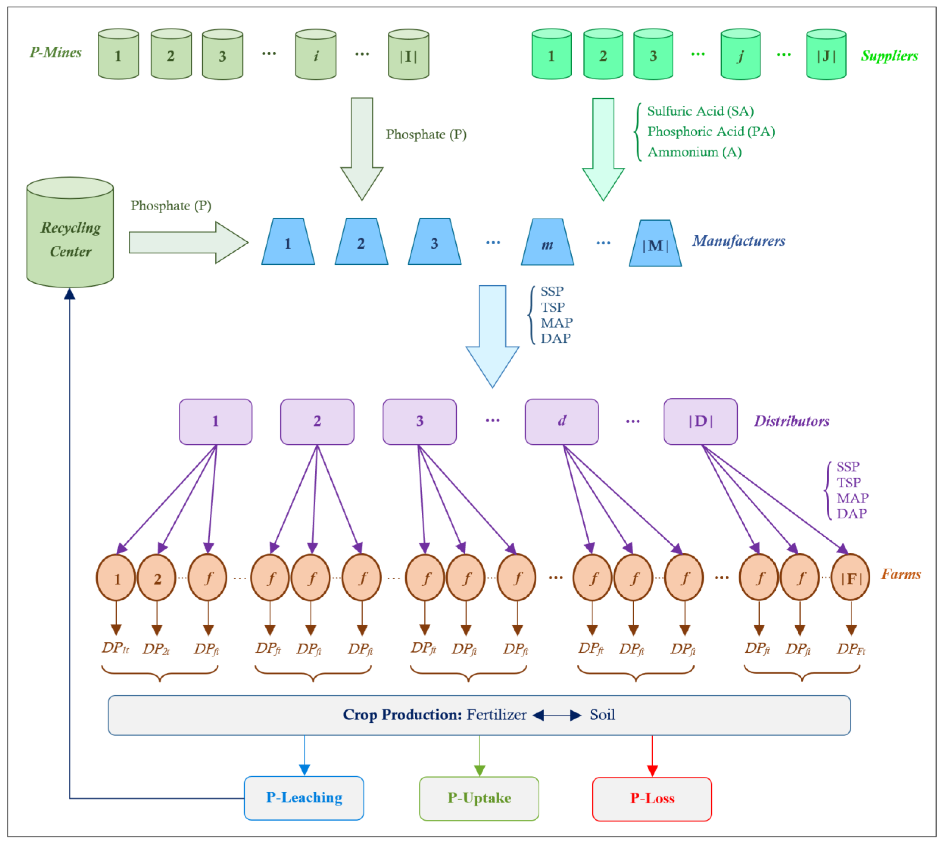
3.1. Supply Chain Network
- P is the main resource of producing P-fertilizers.
- There are three raw materials: SA, PA, and A.
- There are four P-fertilizer products: SSP, TSP, MAP, and DAP.
- To produce a unit of SSP, 0.64 units of P and 0.37 units of SA are used.
- To produce a unit of TSP, 0.4 units of P and 0.34 units of PA are used.
- To produce a unit of MAP, 0.12 units of A and 0.51 units of PA are used.
- To produce a DAP, 0.23 units of A and 0.47 units of PA are consumed.
- PA is considered as a raw material ignoring the production procedure.
- Each manufacturer has a limited capacity to store P-fertilizers.
- Distribution centers can store a part of the received P-fertilizers.
- Lead time of P-recycling is assumed to be one month: the collected P-leaching from farms in each month would be recycled and can be used in the next month.
- Each mine has a limited capacity to provide P each month.
- Each supplier has a specific capacity to provide raw material each month.
- Each manufacturer may produce one, two, three, or four P-fertilizer types, each with a limited capacity.
- The demand of each farm in terms of the total P-uptake and minimum/maximum required level of each type of fertilizer is assumed to be known for every month.
3.2. Notations
3.3. Problem Formulation
3.3.1. Economic Objective Function
3.3.2. Environmental Objective Functions
3.3.3. Multi-Objective Function
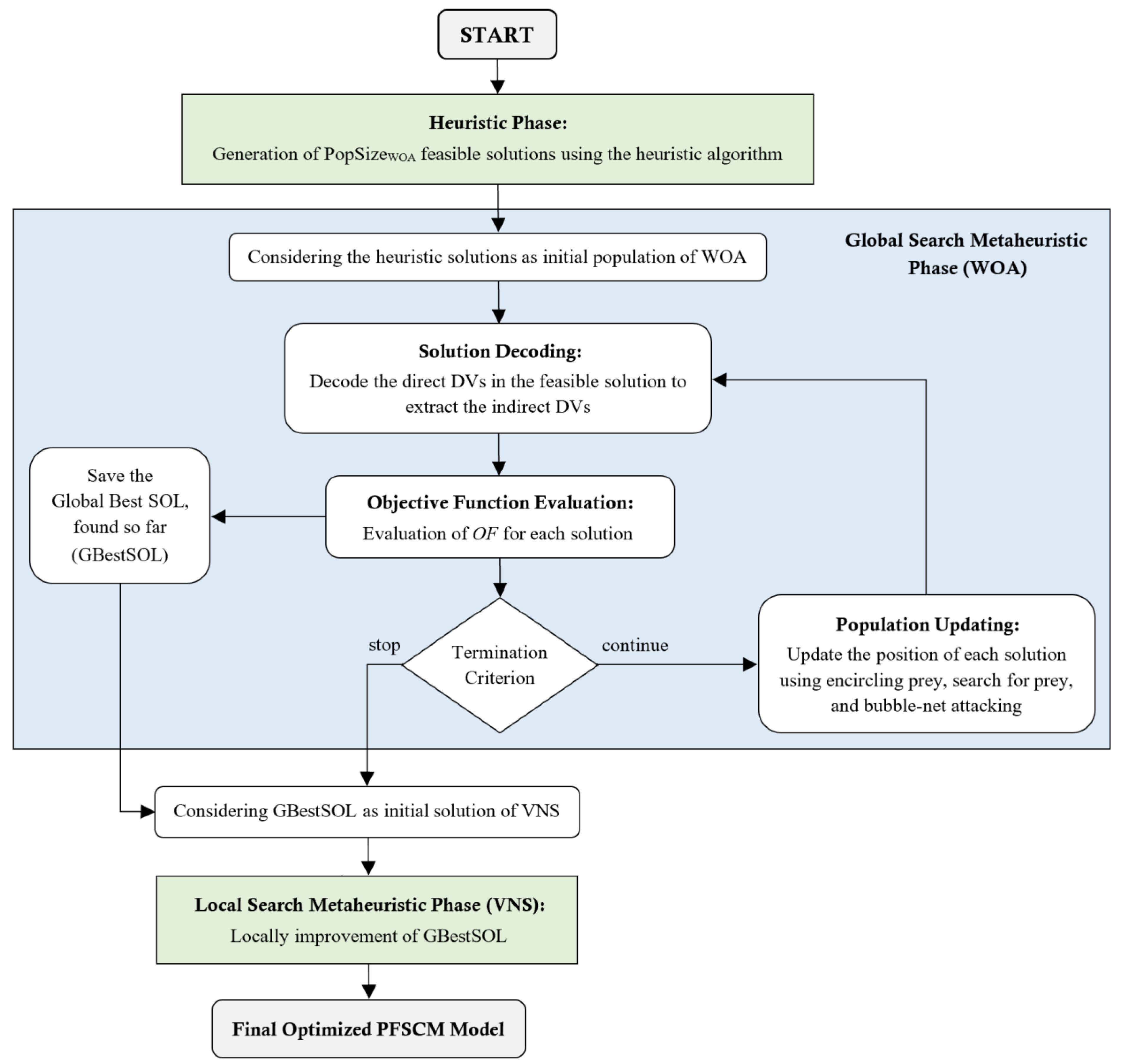
4. Solution Method: H-WOA-VNS
| Algorithm 1. Proposed H-WOA-VNS algorithm for solving the PFSCM problem. |
| Input: |
| Model parameters of the PFSCM model |
| Output: |
| GBestSOL: optimized solution for the PFSCM model |
| Heuristic Phase: |
| 1. for (s ≤ PopSizeWOA) |
| 2. Generate a feasible solution SOL(s) using the heuristic algorithm |
| 3. Add SOL(s) into a population set, s={1,2,…,PopSizeWOA} |
| 4. end for |
| WOA Phase: |
| 1. Considering the heuristic solutions as initial population of WOA |
| 2. for (s ≤ PopSizeWOA) |
| 3. Evaluate the quality of SOL(s) using OF according to Equation (10) |
| 4. end for |
| 5. for1 (n ≤ MaxIterWOA) |
| 6. for2 (s ≤ PopSizeWOA) |
| 7. Update the values of p, l, and , and |
| 8. if1 (p < 0.5) |
| 9. if2 (|| ≥ 1) |
| 10. Update solution s via search for prey as Equation (45) |
| 11. else if2 |
| 12. Update solution s via encircling prey using Equation (46) |
| 13. end if2 |
| 14. else if1 |
| 15. Update solution s via bubble-net attacking using Equation (47) |
| 16. end if1 |
| 17. Revise solution s, if it goes beyond the search space |
| 18. Evaluate the quality of SOL(s) using OF using Equation (10) |
| 19. Updating of the global best solution: GBestSOL |
| 20. end for1 |
| VNS Phase: |
| 1. Considering GBestSOL as initial solution of VNS: SOLcurrent |
| 2. for1 (n ≤ MaxIterVNS) |
| 3. for2 (l ≤ NumLSVNS) |
| 4. Generate SOLnew in vicinity of SOLcurrent via local search operator l |
| 5. Evaluate the quality of SOLnew using OF using Equation (10) |
| 6. if MoFnew<MoFcurrent |
| 7. Replace SOLcurrent with SOLnew |
| 8. Replace MoFcurrent with MoFnew |
| 9. Break for2 |
| 10. end if |
| 11. end for2 |
| 12. Updating of the global best solution: GBestSOL |
| 13. end for1 |
| Output: Return the GBestSOL as the final optimized PFSCM model |
4.1. Solution Representation
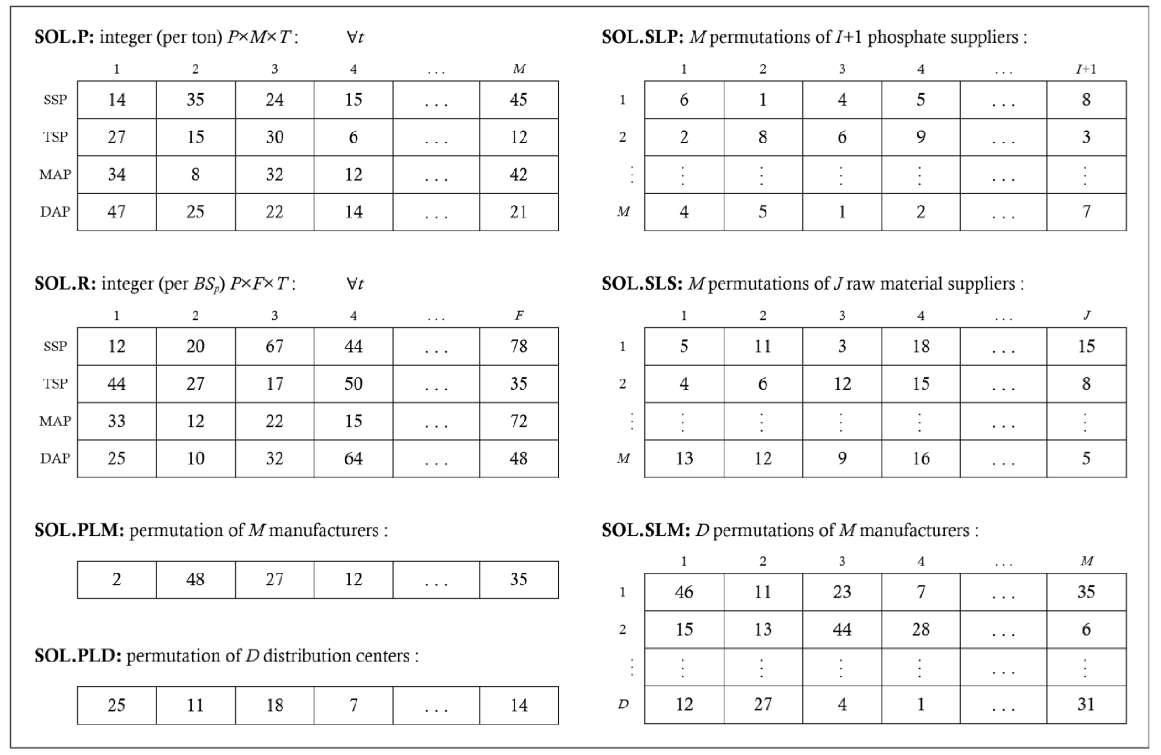
4.1.1. Solution Encoding
- SOL.P () is an integer matrix of dimension P×M×T, which determines the amount of fertilizer p which is produced in manufacturer m at time t (per ton).
- SOL.R () is an integer matrix of dimension P×F×T to determine the amount of each fertilizer p delivered from the corresponding distribution center to each farm f at every time period t (per BSp).
- SOL.PLM () is a permutation of M manufacturers to determine the priority of the manufacturers to order from different P-mines and suppliers.
- SOL.SLP () is a matrix of dimension M×(I + 1) comprising M permutation vectors of I + 1 P suppliers, i.e., each row m is a permutation of I mines plus the recycling center, which determines the selection list of the different P-mines for the manufacturer m.
- SOL.SLS () is a matrix of dimension M×J, where each row m specifies selection list of the different suppliers to supply raw materials for the manufacturer m.
- SOL.PLD () is a permutation of D distribution centers which determines priority of them in ordering fertilizers from the different manufacturers.
- SOL.SLM () is a matrix of dimension D×M, where each row d is a permutation of M manufacturers to determine the selection list of the different manufacturers for the distributor d.
4.1.2. Solution Decoding
- Decoding of farms-distribution centers DVs: in the first step, and are obtained according to the requested demands stored in as:
- Decoding of farms-recycling center DVs: at the end of each time period, after delivering fertilizers to the farm f and the irrigation procedure, the amount of P-leaching for fertilizer p can be estimated by multiplying the total recyclable fertilizers to the P-leaching coefficient of fertilizer p, according to Equation (37). Then, the total amount of recycled phosphate at the end of time t is achieved according to Equation (39). It should be emphasized that the lead time of P recycling is one month, and consequently, the recycled P at time t can be transferred to the manufacturers in times t+1, t+2, and so on. To this end, the values of , , and , are extracted:
- Decoding of distribution centers–manufacturers DVs: Based on the received demands by the farms, the total demand of each distribution center d for each fertilizer p at every time period t is calculated according to Equation (40). Then, the different distributors are given one by one according to their priorities in . For each distribution center d, different manufacturers according to their selection list in are evaluated one by one to deliver fertilizers to the distributor d until satisfying its total demand . As a result, the values of , , and are extracted:
- Decoding of manufacturers–raw material suppliers DVs: Every time t, the demand of each raw material r for each manufacturer m for the production of fertilizer p can be calculated by multiplying to the amount of the produced fertilizer p according to Equation (41). Accordingly, the total demand of raw material r for each manufacturer m at every time t is obtained by Equation (42). Then, to satisfy the demand of the manufacturers, they are evaluated one by one based on their priorities in . The manufacturer m may be sourced by different suppliers according to their selection list in until satisfying the total demand of the manufacturer m for raw materials. As a result, , , , and , are obtained:
- Decoding of manufacturers–phosphate suppliers DVs: The phosphate demand of each manufacturer m to produce the fertilizer p at every time period t can be expressed as in Equation (43), and then, the total phosphate demand for each manufacturer m at every time t is calculated according to Equation (44). Similar to the supplier selection, to satisfy the P demand of the manufacturer m, different P-mines as well as the recycling center (I + 1 phosphate suppliers) are evaluated one by one based on their selection list in until satisfying the phosphate demand of the manufacturer m. To this end, , , , , , and are achieved:
- Decoding of inventories: At the end of each time period t, the inventory of distribution centers, manufacturers, and recycling center, are updated according to Equations (18), (25) and (33), respectively.
4.2. Initialization Using a Heuristic Algorithm
- At first, SOL.R is constructed using the P-uptake demand and minimum/maximum requested fertilizers by the farms. More specifically, the demand of farm f for the fertilizer p at every time period t, , is randomly generated within [LPfpt,UPfpt] to satisfy Equation (12), while the total P-uptake from the different fertilizers fulfills the total demand given in Equation (11).
- The total demand of each distribution center for all fertilizers at all time periods is calculated by the summation of the demands of the corresponding farms. Then, the priority list of the different distribution centers (SOL.PLD) is obtained by sorting them from the highest demand to the lowest demand.
- For each distribution center d, different manufacturers are sorted according to the total cost per unit of fertilizers (including purchasing and transportation costs), from the lowest to the highest cost. This procedure is repeated for all distribution centers to construct SOL.SLM.
- The amount of fertilizer p produced by manufacturer m at time t is considered to be a random value within [0.5 × ,] to construct SOL.P.
- The priority list of the manufacturers (SOL.PLM) is determined by sorting them from the most significant to the least significant according to their total production at all time periods.
- For each manufacturer m, the different raw material suppliers are sorted according to the total cost of purchasing and transportation from the lowest to the highest cost, and eventually, SOL.SLS is obtained. The same procedure is repeated for the I + 1 phosphate suppliers (P-mines plus the recycling center) to construct SOL.SLP.
4.3. Global Search Using WOA
4.3.1. Search for Prey
4.3.2. Encircling Prey
4.3.3. Bubble-Net Attack
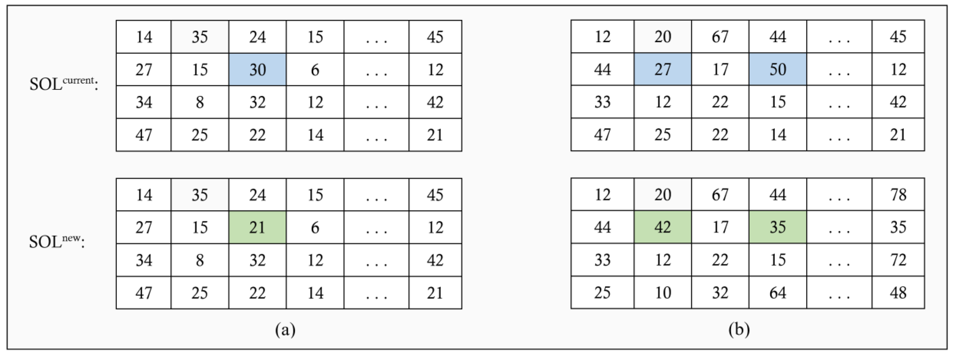
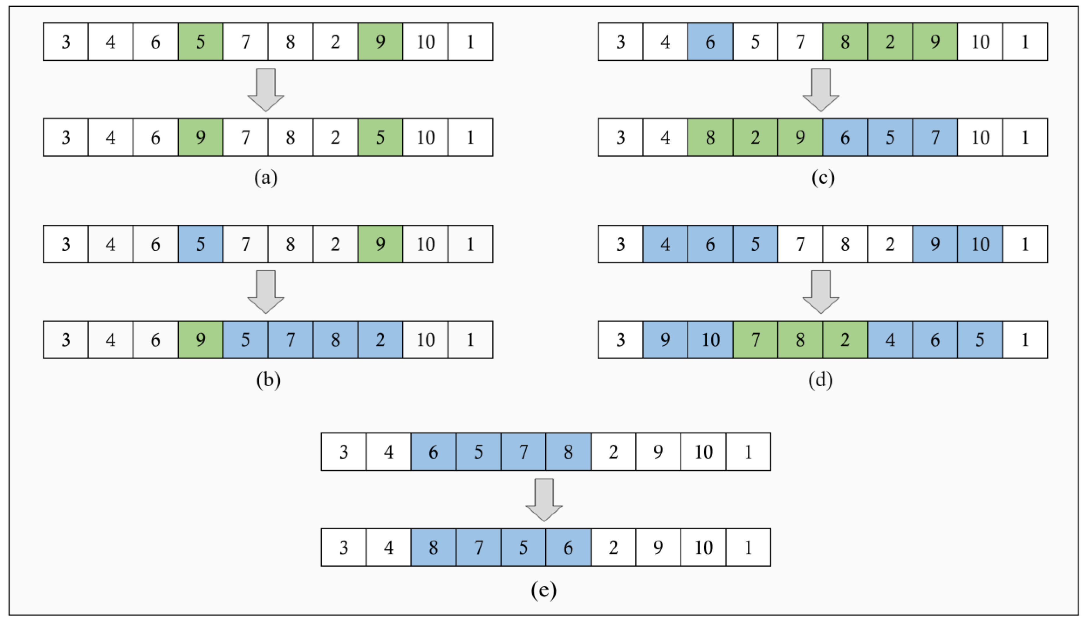
4.4. Local Search Using VNS
5. Experimental Results
5.1. Case Study
5.2. Settings
5.3. Results
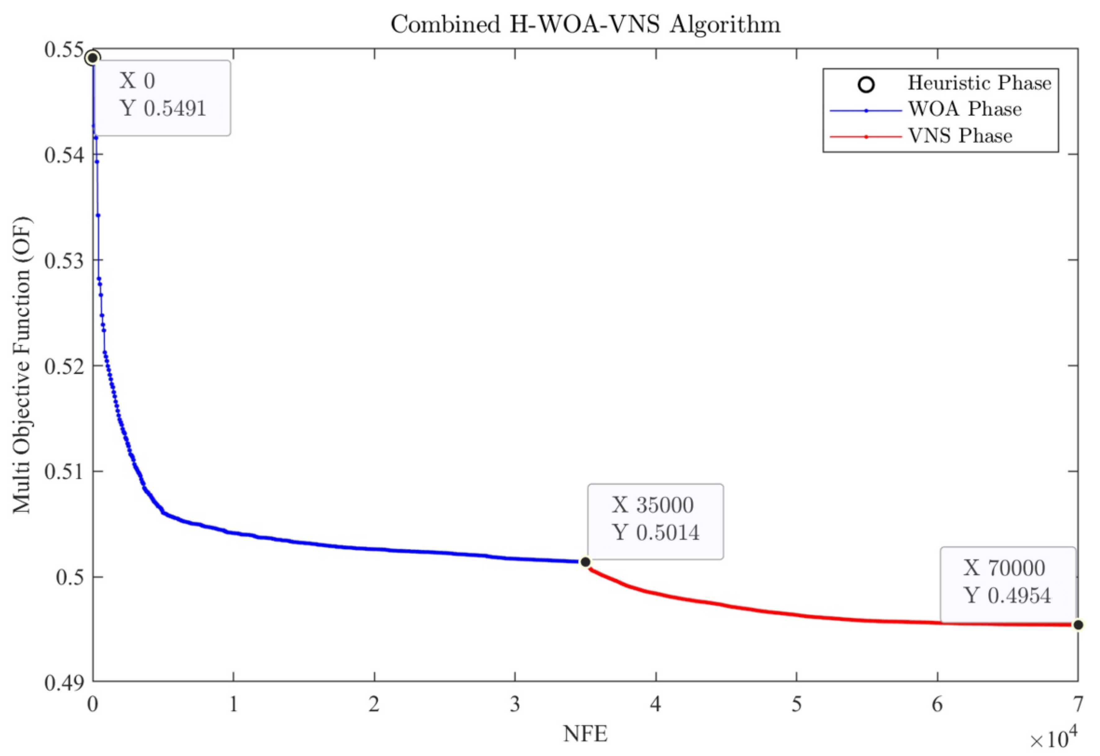
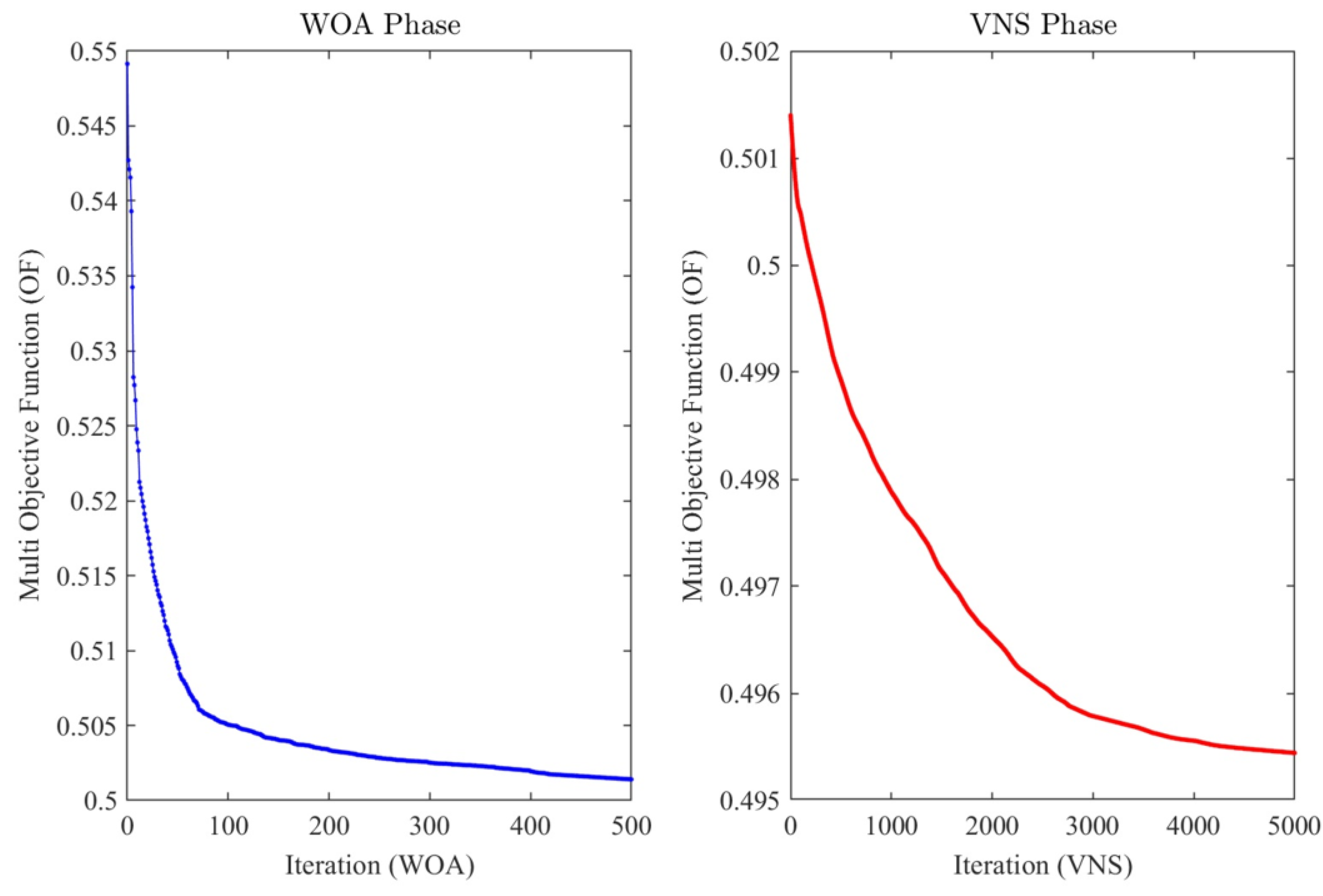
5.3.1. Optimization Results
5.3.2. PFSCM Results
5.4. Validation
5.4.1. Validation of H-WOA-VNS against the Exact Method
5.4.2. Validation of H-WOA-VNS against Other Heuristics and Metaheuristics
5.5. Discussion
5.6. Managerial Insights
6. Conclusions
Author Contributions
Funding
Institutional Review Board Statement
Informed Consent Statement
Data Availability Statement
Conflicts of Interest
References
- Huang, H.; Li, J.; Li, B.; Zhang, D.; Zhao, N.; Tang, S. Comparison of different K-struvite crystallization processes for simultaneous potassium and phosphate recovery from source-separated urine. Sci. Total Environ. 2019, 651, 787–795. [Google Scholar] [CrossRef]
- Nedelciu, C.E.; Ragnarsdottir, K.V.; Schlyter, P.; Stjernquist, I. Global phosphorus supply chain dynamics: Assessing regional impact to 2050. Glob. Food Secur. 2020, 26, 100426. [Google Scholar] [CrossRef]
- Barbosa, M.W. Uncovering research streams on agri-food supply chain management: A bibliometric study. Glob. Food Secur. 2021, 28, 100517. [Google Scholar] [CrossRef]
- Kang, S.; Kim, G.; Roh, J.; Jeon, E.C. Ammonia Emissions from NPK Fertilizer Production Plants: Emission Characteristics and Emission Factor Estimation. Int. J. Environ. Res. Public Health 2022, 19, 6703. [Google Scholar] [CrossRef]
- Shokouhifar, M. FH-ACO: Fuzzy heuristic-based ant colony optimization for joint virtual network function placement and routing. Appl. Soft Comput. 2021, 107, 107401. [Google Scholar] [CrossRef]
- Al-Qaness, M.A.; Ewees, A.A.; Fan, H.; Abd Elaziz, M. Optimized forecasting method for weekly influenza confirmed cases. Int. J. Environ. Res. Public Health 2020, 17, 3510. [Google Scholar] [CrossRef]
- Khairunissa, M.; Lee, H. Hybrid Metaheuristic-Based Spatial Modeling and Analysis of Logistics Distribution Center. ISPRS Int. J. Geo-Inf. 2022, 11, 5. [Google Scholar] [CrossRef]
- Shokouhifar, M.; Ranjbarimesan, M. Multivariate time-series blood donation/demand forecasting for resilient supply chain management during COVID-19 pandemic. Clean. Logist. Supply Chain 2022, 5, 100078. [Google Scholar] [CrossRef]
- Shehadeh, H.A.; Mustafa, H.M.J.; Tubishat, M. A Hybrid Genetic Algorithm and Sperm Swarm Optimization (HGASSO) for Multimodal Functions. Int. J. Appl. Metaheuristic Comput. (IJAMC) 2022, 13, 1–33. [Google Scholar] [CrossRef]
- Ilinova, A.; Dmitrieva, D.; Kraslawski, A. Influence of COVID-19 pandemic on fertilizer companies: The role of competitive advantages. Resour. Policy 2021, 71, 102019. [Google Scholar] [CrossRef]
- Rabbani, M.; Molana, S.M.H.; Sajadi, S.M.; Davoodi, M.H. Sustainable fertilizer supply chain network design using evolutionary-based resilient robust stochastic programming. Comput. Ind. Eng. 2022, 174, 108770. [Google Scholar] [CrossRef]
- Scholz, R.W.; Ulrich, A.E.; Eilittä, M.; Roy, A. Sustainable use of phosphorus: A finite resource. Sci. Total Environ. 2013, 461, 799–803. [Google Scholar] [CrossRef]
- Gong, H.; Meng, F.; Wang, G.; Hartmann, T.E.; Feng, G.; Wu, J.; Jiao, X.; Zhang, F. Toward the sustainable use of mineral phosphorus fertilizers for crop production in China: From primary resource demand to final agricultural use. Sci. Total Environ. 2022, 804, 150183. [Google Scholar] [CrossRef]
- Godde, C.M.; Mason-D’Croz, D.; Mayberry, D.E.; Thornton, P.K.; Herrero, M. Impacts of climate change on the livestock food supply chain; a review of the evidence. Glob. Food Secur. 2021, 28, 100488. [Google Scholar] [CrossRef]
- Yu, X.; Keitel, C.; Dijkstra, F.A. Global analysis of phosphorus fertilizer use efficiency in cereal crops. Glob. Food Secur. 2021, 29, 100545. [Google Scholar] [CrossRef]
- Withers, P.J.A.; Sylvester-Bradley, R.; Jones, D.L.; Healey, J.R.; Talboys, P.J. Feed the Crop not the Soil: Rethinking Phosphorus Management in the Food Chain; ACS Publications: Washington, DC, USA, 2014. [Google Scholar]
- Gaffney, J.; Bing, J.; Sawyer, J.; Byrne, P.; Cassman, K.; Ciampitti, I.; Warner, D. Science-based intensive agriculture: Sustainability, food security, and the role of technology. Glob. Food Secur. 2019, 23, 236–244. [Google Scholar] [CrossRef]
- Chowdhury, R.B.; Moore, G.A.; Weatherley, A.J.; Arora, M. A novel substance flow analysis model for analysing multi-year phosphorus flow at the regional scale. Sci. Total Environ. 2016, 572, 1269–1280. [Google Scholar] [CrossRef]
- Gurevitch, J.; Koricheva, J.; Nakagawa, S.; Stewart, G. Meta-analysis and the science of research synthesis. Nature 2018, 555, 175–182. [Google Scholar] [CrossRef]
- De Oliveira, A.K.S.; Soares, E.B.; dos Santos, M.G.; Lins, H.A.; de Freitas Souza, M.; dos Santos Coêlho, E.; Silveira, L.M.; Mendonça, V.; Barros Júnior, A.P.A.; de Araújo de Araújo Rangel Lopes, W. Efficiency of Phosphorus Use in Sunflower. Agronomy 2022, 12, 1558. [Google Scholar] [CrossRef]
- Tabbassum, R.; Naveed, M.; Mehboob, I.; Babar, M.H.; Holatko, J.; Akhtar, N.; Rafique, M.; Kucerik, J.; Brtnicky, M.; Kintl, A. Comparative Response of Fermented and Non-Fermented Animal Manure Combined with Split Dose of Phosphate Fertilizer Enhances Agronomic Performance and Wheat Productivity through Enhanced P Use Efficiency. Agronomy 2022, 12, 2335. [Google Scholar] [CrossRef]
- Fakhravar, H. Combining heuristics and Exact Algorithms: A Review. arXiv 2022, arXiv:2202.02799. [Google Scholar]
- Tirkolaee, E.B.; Goli, A.; Ghasemi, P.; Goodarzian, F. Designing a sustainable closed-loop supply chain network of face masks during the COVID-19 pandemic: Pareto-based algorithms. J. Clean. Prod. 2022, 333, 130056. [Google Scholar] [CrossRef]
- Sohrabi, M.; Zandieh, M.; Afshar-nadjafi, B. A simple empirical inventory model for managing with demand differentiation. Comput. Appl. Math. 2021, 40, 1–38. [Google Scholar] [CrossRef]
- Sohrabi, M.; Zandieh, M.; Nadjafi, B.A. Dynamic demand-centered process-oriented data model for inventory management of hemovigilance systems. Healthc. Inform. Res. 2021, 27, 73–81. [Google Scholar] [CrossRef]
- Shokouhifar, M. Swarm intelligence RFID network planning using multi-antenna readers for asset tracking in hospital environments. Comput. Netw. 2021, 198, 108427. [Google Scholar] [CrossRef]
- Rajabi Moshtaghi, H.; Toloie Eshlaghy, A.; Motadel, M.R. A comprehensive review on meta-heuristic algorithms and their classification with novel approach. J. Appl. Res. Ind. Eng. 2021, 8, 63–89. [Google Scholar]
- Farag, M.A.; El-Shorbagy, M.A.; Mousa, A.A.; El-Desoky, I.M. A new hybrid metaheuristic algorithm for multiobjective optimization problems. Int. J. Comput. Intell. Syst. 2020, 13, 920. [Google Scholar] [CrossRef]
- Chouhan, V.K.; Khan, S.H.; Hajiaghaei-Keshteli, M. Metaheuristic approaches to design and address multi-echelon sugarcane closed-loop supply chain network. Soft Comput. 2021, 25, 11377–11404. [Google Scholar] [CrossRef]
- Gholizadeh, H.; Goh, M.; Fazlollahtabar, H.; Mamashli, Z. Modelling uncertainty in sustainable-green integrated reverse logistics network using metaheuristics optimization. Comput. Ind. Eng. 2022, 163, 107828. [Google Scholar] [CrossRef]
- Karmakar, S.; Kundu, A.; John, B. Optimizing a Supply Chain Network Using Metaheuristic for Pre and Post Pandemic Scenario. In Proceedings of the 2021 IEEE International Conference on Industrial Engineering and Engineering Management (IEEM), Singapore, 13–16 December 2021; pp. 41–45. [Google Scholar]
- Nath, M.P.; Priyadarshini, S.B.B.; Mishra, D. Supply chain management (SCM): Employing various big data and metaheuristic strategies. In Advances in Machine Learning for Big Data Analysis; Springer: Berlin/Heidelberg, Germany, 2022; pp. 145–165. [Google Scholar]
- Nahavandi, B.; Homayounfar, M.; Daneshvar, A.; Shokouhifar, M. Hierarchical structure modelling in uncertain emergency location-routing problem using combined genetic algorithm and simulated annealing. Int. J. Comput. Appl. Technol. 2022, 68, 150–163. [Google Scholar] [CrossRef]
- Wu, W.; Zhou, W.; Lin, Y.; Xie, Y.; Jin, W. A hybrid metaheuristic algorithm for location inventory routing problem with time windows and fuel consumption. Expert Syst. Appl. 2021, 166, 114034. [Google Scholar] [CrossRef]
- Shokouhifar, M.; Pilevari, N. Combined adaptive neuro-fuzzy inference system and genetic algorithm for e-learning resilience assessment during COVID-19 pandemic. Concurr. Comput. Pract. Exp. 2022, 34, e6791. [Google Scholar] [CrossRef]
- Liu, Y.; Chen, C. Improved RFM Model for Customer Segmentation Using Hybrid Meta-heuristic Algorithm in Medical IoT Applications. Int. J. Artif. Intell. Tools 2022, 31, 2250009. [Google Scholar] [CrossRef]
- Ghasemi Darehnaei, Z.; Shokouhifar, M.; Yazdanjouei, H.; Rastegar Fatemi, S.M.J. SI-EDTL: Swarm intelligence ensemble deep transfer learning for multiple vehicle detection in UAV images. Concurr. Comput. Pract. Exp. 2022, 34, e6726. [Google Scholar] [CrossRef]
- Shokouhifar, M.; Sabbaghi, M.M.; Pilevari, N. Inventory management in blood supply chain considering fuzzy supply/demand uncertainties and lateral transshipment. Transfus. Apher. Sci. 2021, 60, 103103. [Google Scholar] [CrossRef]
- Naderi, R.; Shafiei Nikabadi, M.; Alem Tabriz, A.; Pishvaee, M.S. Supply chain sustainability improvement using exergy analysis. Comput. Ind. Eng. 2021, 154, 107142. [Google Scholar] [CrossRef]
- Sohrabi, M.; Zandieh, M.; Shokouhifar, M. Sustainable inventory management in blood banks considering health equity using a combined metaheuristic-based robust fuzzy stochastic programming. Socio. -Econ. Plan. Sci. 2022. In press. [Google Scholar] [CrossRef]
- Sörensen, K. Metaheuristics—The metaphor exposed. Int. Trans. Oper. Res. 2015, 22, 3–18. [Google Scholar] [CrossRef]
- Esmaeili, H.; Hakami, V.; Bidgoli, B.M.; Shokouhifar, M. Application-specific clustering in wireless sensor networks using combined fuzzy firefly algorithm and random forest. Expert Syst. Appl. 2022, 210, 118365. [Google Scholar] [CrossRef]
- Shokouhifar, M.; Jalali, A. Optimized sugeno fuzzy clustering algorithm for wireless sensor networks. Eng. Appl. Artif. Intell. 2017, 60, 16–25. [Google Scholar] [CrossRef]
- Mirjalili, S.; Lewis, A. The whale optimization algorithm. Adv. Eng. Softw. 2016, 95, 51–67. [Google Scholar] [CrossRef]
- Wang, K.M.; Wang, K.J.; Chen, C.C. Capacitated production planning by parallel genetic algorithm for a multi-echelon and multi-site TFT-LCD panel manufacturing supply chain. Appl. Soft Comput. 2022, 127, 109371. [Google Scholar] [CrossRef]
- Fathollahi-Fard, A.M.; Govindan, K.; Hajiaghaei-Keshteli, M.; Ahmadi, A. A green home health care supply chain: New modified simulated annealing algorithms. J. Clean. Prod. 2019, 240, 118200. [Google Scholar] [CrossRef]


| Sets and Indices | Definition |
|---|---|
| i ∊I | Set of P-mines (suppliers of phosphorus) |
| j ∊J | Set of suppliers of raw materials |
| m ∊M | Set of manufacturers |
| d ∊D | Set of distributors |
| f ∊F | Set of farms (demand nodes) |
| t ∊T | Set of months (time periods) |
| r ∊R | Set of raw materials: A (r = 1), PA (r = 2), and SA (r = 3) |
| p ∊P | Set of products: SSP (p = 1), TSP (p = 2), MAP (p = 3), and DAP (p = 4) |
| Parameters | Definition |
| 1 if farm f is supported by distribution center d; 0 otherwise | |
| Batch size of ordering fertilizer p by farms (ton) | |
| Capacity of supplying P by mine i in time t (ton) | |
| Capacity of supplier j to supply raw material r in time t (ton) | |
| Capacity of manufacturer m to produce fertilizer p in each time (ton) | |
| Warehouse capacity of manufacturer m (ton) | |
| Warehouse capacity of distribution center d (ton) | |
| Warehouse capacity of recycling center (ton) | |
| Required P rock to produce unit fertilizer p (%) | |
| Required raw material r for the production of unit fertilizer p (%) | |
| Phosphorus uptake by farm f from unit fertilizer p (%) | |
| Crop yield increase in farm f from unit fertilizer p (%) | |
| Recyclable phosphorus in farm f from unit fertilizer p (%) | |
| Total phosphorus loss to produce a unit of fertilizer p (%) | |
| Amount of recyclable P per unit P-leaching of fertilizer p (%) | |
| Phosphorus demand by farm f in time period t (ton) | |
| Minimum amount of fertilizer p which should be delivered to farm f in time t (ton) | |
| Maximum amount of fertilizer p which should be delivered to farm f in time t (ton) | |
| Transportation cost of carrying phosphorus from mine i to manufacturer m (USD/ton) | |
| Transportation cost of carrying phosphorus from recycling center to manufacturer m (USD/ton) | |
| Transportation cost from supplier j to manufacturer m for carrying raw materials (USD/ton) | |
| Transportation cost of carrying fertilizers from manufacturer m to distribution center d (USD/ton) | |
| Transportation cost of carrying fertilizers from distribution center d to farm f (USD/ton) | |
| Transportation cost of carrying phosphorus leaching from farm f to recycling center (USD/ton) | |
| Purchasing cost of phosphate from mine i (USD/ton) | |
| Purchasing cost from supplier j for raw material r (USD/ton) | |
| Production cost in manufacturer m for unit fertilizer p (USD/ton) | |
| Recycling cost of unit P in recycling center (USD/ton) | |
| Initial inventory of fertilizer p in manufacturer m (ton) | |
| Inventory cost in manufacturer m for each month (USD/ton/month) | |
| Inventory cost in distribution center d for each month (USD/ton/month) | |
| Inventory cost in recycling center for each month (USD/ton/month) | |
| Direct DVs | Definition |
| Amount of fertilizer p produced in time t by manufacturer j (ton) | |
| Amount of fertilizer p delivered in time t to farm f (BSp) | |
| Priority list of manufacturers determining their order in P-mine and supplier assignment | |
| Selection list of P-mines (plus recycling center) for manufacturer m | |
| Selection list of suppliers for manufacturer m | |
| Priority list of distributors determining the order of distributors in manufacturer assignment | |
| Selection list of manufacturers for distributor d | |
| Indirect DVs | Definition |
| Required amount of raw material r in manufacturer m to produce fertilizer p in time t (ton) | |
| Required raw material r in manufacturer m to produce all fertilizers in time t (ton) | |
| Total P recycled at time t (ton) | |
| Total demand of fertilizer p in distribution center d in time t (ton) | |
| 1 if mine i supplies P for manufacturer m in time t; 0 otherwise | |
| 1 if the recycling center supplies P to manufacturer m in time t; 0 otherwise | |
| 1 if supplier j supplies raw material r to manufacturer m in time t; 0 otherwise | |
| 1 if fertilizer p is delivered from manufacturer m to distribution center d in time t; 0 otherwise | |
| 1 if fertilizer p is delivered from distribution center d to farm f in time t; 0 otherwise | |
| 1 if P-leaching of fertilizer p is delivered from farm f to the recycling center in time t; 0 otherwise | |
| Amount of P delivered in time t from mine i to manufacturer m (ton) | |
| Amount of P transferred in time t from the recycling center to manufacturer m (ton) | |
| Amount of raw material r transferred in time t from supplier j to manufacturer m (ton) | |
| Amount of fertilizer p transferred in time t from manufacturer m to distribution center d (ton) | |
| Amount of fertilizer p transferred in time t from distribution center d to farm f (ton) | |
| Amount of P-leaching of fertilizer p transferred in time t from farm f to the recycling center (ton) | |
| Inventory of manufacturer m for fertilizer p at time t (ton) | |
| Inventory of distribution center d for fertilizer p at time t (ton) | |
| Inventory of recycled P in the recycling center at time t (ton) |
| Distributor | P-Uptake | TSP | MAP | DAP | |||
|---|---|---|---|---|---|---|---|
| Lower | Upper | Lower | Upper | Lower | Upper | ||
| 1 | 25,820 | 9120 | 35,820 | 10,660 | 41,580 | 5570 | 25,380 |
| 2 | 23,130 | 9980 | 33,660 | 12,860 | 41,400 | 7200 | 23,040 |
| 3 | 22,180 | 10,270 | 35,280 | 7200 | 52,020 | 5760 | 19,080 |
| 4 | 17,210 | 6910 | 30,780 | 7780 | 31,860 | 3840 | 13,680 |
| 5 | 8610 | 3260 | 14,220 | 3360 | 13,500 | 2020 | 8460 |
| 6 | 10,260 | 3460 | 15,300 | 5470 | 22,140 | 2590 | 8640 |
| 7 | 2810 | 1340 | 4860 | 1440 | 4680 | 670 | 2700 |
| 8 | 7260 | 1540 | 12,600 | 4220 | 13,320 | 1630 | 6480 |
| 9 | 5140 | 1920 | 7920 | 2780 | 8640 | 1440 | 4320 |
| 10 | 5810 | 2590 | 8460 | 1820 | 9900 | 1540 | 5940 |
| 11 | 41,330 | 14,500 | 70,020 | 17,860 | 66,240 | 11,620 | 42,300 |
| 12 | 10,760 | 3170 | 20,160 | 4900 | 19,980 | 2590 | 11,160 |
| 13 | 52,810 | 20,740 | 97,200 | 26,400 | 92,340 | 13,630 | 47,520 |
| 14 | 12,180 | 6530 | 24,120 | 4800 | 20,880 | 2880 | 10,980 |
| 15 | 4350 | 1730 | 5400 | 2300 | 7560 | 1250 | 3420 |
| 16 | 9810 | 4700 | 16,020 | 5660 | 19,800 | 2020 | 10,440 |
| 17 | 37,270 | 14,590 | 68,400 | 14,780 | 59,940 | 7010 | 32,760 |
| 18 | 15,000 | 5660 | 22,500 | 5570 | 28,080 | 3740 | 11,700 |
| 19 | 4180 | 1920 | 6120 | 2020 | 8100 | 580 | 3780 |
| 20 | 19,200 | 7680 | 32,760 | 8830 | 33,120 | 4320 | 19,080 |
| 21 | 15,410 | 6430 | 25,380 | 7580 | 28,440 | 2400 | 12,960 |
| 22 | 24,670 | 14,300 | 46,980 | 12,770 | 46,980 | 5470 | 26,100 |
| 23 | 4530 | 2020 | 7380 | 1340 | 7920 | 1250 | 4860 |
| 24 | 25,050 | 11,140 | 40,680 | 9310 | 52,020 | 5470 | 22,680 |
| 25 | 16,460 | 6910 | 24,840 | 7680 | 31,860 | 3360 | 15,300 |
| 26 | 20,360 | 9120 | 34,560 | 6620 | 30,780 | 4420 | 17,820 |
| 27 | 11,090 | 4510 | 19,980 | 4990 | 21,060 | 2400 | 10,800 |
| 28 | 9610 | 4030 | 13,500 | 4510 | 17,100 | 2400 | 8640 |
| 29 | 6830 | 3550 | 10,440 | 3940 | 10,980 | 2110 | 7740 |
| 30 | 19,480 | 7100 | 33,300 | 8930 | 36,000 | 4220 | 18,540 |
| 31 | 3560 | 1340 | 5580 | 1250 | 5940 | 860 | 3600 |
| 32 | 13,840 | 6430 | 21,240 | 7100 | 21,600 | 2590 | 13,860 |
| Sum | 506,010 | 208,490 | 845,460 | 226,730 | 905,760 | 118,850 | 473,760 |
| P-Fertilizer | PA | SA | A | P |
|---|---|---|---|---|
| SSP | 0 | 64 | 0 | 64 |
| TSP | 34 | 40 | 0 | 40 |
| MAP | 51 | 0 | 12 | 0 |
| DAP | 47 | 0 | 23 | 0 |
| Raw Material | Minimum Capacity | Maximum Capacity | Total Capacity |
|---|---|---|---|
| PA | 12,000 | 240,000 | 870,000 |
| SA | 15,000 | 620,000 | 3,420,000 |
| A | 18,000 | 1,550,000 | 6,200,000 |
| P | 80,000 | 250,000 | 830,000 |
| Manufacturer | SSP | TSP | MAP | DAP |
|---|---|---|---|---|
| 1 | 15,000 | 5000 | 9100 | 11,860 |
| 2 | 6660 | 13,340 | 11,000 | 14,500 |
| 3 | 2500 | 2500 | 2560 | 3400 |
| 4 | 3340 | 3340 | 0 | 0 |
| 5 | 2500 | 1660 | 2480 | 3180 |
| 6 | 2500 | 2500 | 0 | 0 |
| 7 | 3340 | 1660 | 2520 | 3460 |
| 8 | 4160 | 0 | 0 | 0 |
| 9 | 8340 | 5000 | 8160 | 11,320 |
| 10 | 0 | 16,660 | 13,380 | 23,860 |
| 11 | 16,660 | 0 | 21,320 | 29,360 |
| 12 | 0 | 16,660 | 0 | 0 |
| 13 | 10,000 | 2080 | 5640 | 9080 |
| 14 | 2400 | 4500 | 0 | 0 |
| 15 | 8340 | 16,660 | 0 | 0 |
| 16 | 4160 | 840 | 3220 | 3840 |
| 17 | 4160 | 0 | 0 | 0 |
| 18 | 7500 | 2500 | 0 | 0 |
| 19 | 8340 | 8340 | 0 | 0 |
| 20 | 6000 | 6000 | 6360 | 8860 |
| 21 | 3340 | 1500 | 0 | 0 |
| Sum | 119,240 | 110,740 | 85,740 | 122,720 |
| Phase | Parameter | Value/Description |
|---|---|---|
| Heuristic | Maximum Iterations (MaxIterWOA) | 70 (=PopSizeWOA) |
| WOA | Population Size (PopSizeWOA) | 500 |
| Population updating mechanisms | 70 | |
| Maximum Iterations (MaxIterVNS) | Encircling prey, Search for prey, Bubble-net attack | |
| VNS | Number of Local Search operators (NumLSVNS) | 5000 |
| Local search operators | 7 | |
| Weight of economic cost (wEC) | I-Swap, I-Exchange, Exchange, Relocate, OrOpt, TwoOpt, and Reverse | |
| OF weights | Weight of crop yield (wCY) | 0.5 |
| Maximum Iterations (MaxIterWOA) | 0.3 | |
| Weight of PUE (wPUE) | 0.2 |
| (a) Purchasing Cost of the Raw Materials (USD/ton) | ||||
|---|---|---|---|---|
| Raw Material | PA | SA | A | P |
| Purchasing cost | 310~370 | 60~70 | 20~25 | 80~95 |
| (b) Production cost of P-fertilizers (USD/ton) | ||||
| Fertilizer | SSP | TSP | MAP | DAP |
| Production cost | 110~130 | 120~150 | 210~250 | 230~280 |
| (c) P-fertilizers coefficients (%) | ||||
| Parameter | SSP | TSP | MAP | DAP |
| 0.26~0.32 | 0.29~0.35 | 0.42~0.47 | 0.46~0.52 | |
| 0.21~0.28 | 0.24~0.3 | 0.38~0.46 | 0.45~0.51 | |
| 0.23~0.27 | 0.21~0.27 | 0.12~0.17 | 0.16~0.2 | |
| 0.53 | 0.38 | 0.64 | 0.62 | |
| 0.09 | 0.1 | 0.07 | 0.06 | |
| (d) Other parameters | ||||
| Parameter | Value | Parameter | Value | |
| 1 (ton) | 1.5~2 (USD/truck/km) | |||
| Truck size | 25 (ton) | 1.5~2 (USD/truck /km) | ||
| 20 (USD/ton) | 2~3 (USD/truck /km) | |||
| 1.5 (USD/ton/month) | 2~2.5 (USD/truck /km) | |||
| 2.5 (USD/ton/month) | 2~2.5 (USD/truck /km) | |||
| 2 (USD/ton/month) | 2.5~3 (USD/truck /km) | |||
| Run | Total Cost (M$) | PF | OF | |||
|---|---|---|---|---|---|---|
| 1 | 451.81 | 0.3012 | 0.3291 | 0.2789 | 0 | 0.4961 |
| 2 | 454.39 | 0.3029 | 0.33 | 0.278 | 0 | 0.4969 |
| 3 | 451.87 | 0.3012 | 0.3313 | 0.2778 | 0 | 0.4957 |
| 4 | 446.38 | 0.2976 | 0.3302 | 0.2781 | 0 | 0.4941 |
| 5 | 449.97 | 0.3 | 0.3317 | 0.2776 | 0 | 0.495 |
| 6 | 450.4 | 0.3003 | 0.3303 | 0.278 | 0 | 0.4954 |
| 7 | 448.04 | 0.2987 | 0.3303 | 0.2777 | 0 | 0.4947 |
| 8 | 453.47 | 0.3023 | 0.3298 | 0.2779 | 0 | 0.4966 |
| 9 | 449.1 | 0.2994 | 0.3295 | 0.2786 | 0 | 0.4951 |
| 10 | 446.55 | 0.2977 | 0.3293 | 0.2785 | 0 | 0.4944 |
| Worst | 454.39 | 0.3029 | 0.3291 | 0.2776 | 0 | 0.4969 |
| Best | 446.38 | 0.2976 | 0.3317 | 0.2789 | 0 | 0.4941 |
| Mean | 450.2 | 0.3001 | 0.3301 | 0.2781 | 0 | 0.4954 |
| STD% | 0.61 | 0.61 | 0.25 | 0.15 | 0 | 0.19 |
| Function | CPP | CPS | CPR | CRC | CIH | CTR | Total (ZEC) |
|---|---|---|---|---|---|---|---|
| Cost (M$) | 12.45 | 118.68 | 178.73 | 8.43 | 25.23 | 102.86 | 446.38 |
| Manufacturer | SSP | TSP | MAP | DAP |
|---|---|---|---|---|
| 1 | 62,201 | 16,814 | 23,755 | 13,767 |
| 2 | 20,880 | 34,684 | 24,411 | 29,242 |
| 3 | 3443 | 6301 | 7610 | 10,408 |
| 4 | 10,603 | 13,513 | 0 | 0 |
| 5 | 9711 | 7485 | 7930 | 3633 |
| 6 | 6847 | 6915 | 0 | 0 |
| 7 | 12,862 | 4020 | 4287 | 7042 |
| 8 | 11,579 | 0 | 0 | 0 |
| 9 | 36,142 | 19,016 | 28,027 | 4825 |
| 10 | 0 | 40,030 | 27,374 | 29,133 |
| 11 | 55,695 | 0 | 65,218 | 52,210 |
| 12 | 0 | 29,818 | 0 | 0 |
| 13 | 24,000 | 7365 | 20,805 | 6362 |
| 14 | 4521 | 17,704 | 0 | 0 |
| 15 | 10,999 | 54,914 | 0 | 0 |
| 16 | 10,259 | 2594 | 5161 | 10,004 |
| 17 | 14,697 | 0 | 0 | 0 |
| 18 | 16,603 | 8301 | 0 | 0 |
| 19 | 12,711 | 35,751 | 0 | 0 |
| 20 | 12,264 | 24,220 | 15,398 | 19,173 |
| 21 | 9984 | 4688 | 0 | 0 |
| Total | 346,001 | 334,133 | 229,976 | 185,799 |
| P-Fertilizer | PA | SA | A | P |
|---|---|---|---|---|
| SSP | 0 | 128,020 | 0 | 221,441 |
| TSP | 113,605 | 0 | 0 | 133,653 |
| MAP | 117,288 | 0 | 27,597 | 0 |
| DAP | 87,326 | 0 | 42,734 | 0 |
| Total | 318,219 | 128,020 | 70,331 | 355,090 |
| Distributor | Delivered P-Fertilizers | P-Uptake | ||||
|---|---|---|---|---|---|---|
| SSP | TSP | MAP | DAP | Demand | Satisfied | |
| 1 | 22,371 | 18,384 | 13,869 | 12,442 | 25,820 | 25,990 |
| 2 | 18,540 | 19,411 | 11,707 | 11,309 | 23,130 | 23,536 |
| 3 | 17,265 | 18,403 | 12,016 | 10,496 | 22,180 | 22,531 |
| 4 | 13,536 | 12,662 | 10,395 | 8235 | 17,210 | 17,542 |
| 5 | 6758 | 7088 | 4386 | 4443 | 8610 | 8806 |
| 6 | 7799 | 8365 | 5305 | 5578 | 10,260 | 10,572 |
| 7 | 2479 | 2193 | 1453 | 1503 | 2810 | 2957 |
| 8 | 5536 | 6286 | 3956 | 3563 | 7260 | 7503 |
| 9 | 4006 | 4292 | 2750 | 2434 | 5140 | 5216 |
| 10 | 4999 | 4402 | 3140 | 2711 | 5810 | 5888 |
| 11 | 33,189 | 37,554 | 19,863 | 19,200 | 41,330 | 42,001 |
| 12 | 8335 | 8105 | 6165 | 5133 | 10,760 | 10,825 |
| 13 | 40,304 | 38,313 | 31,625 | 27,526 | 52,810 | 54,315 |
| 14 | 8791 | 9092 | 6695 | 6465 | 12,180 | 12,234 |
| 15 | 3354 | 3489 | 2418 | 2236 | 4350 | 4490 |
| 16 | 7704 | 7757 | 4956 | 5027 | 9810 | 9891 |
| 17 | 31,447 | 28,598 | 21,209 | 17,344 | 37,270 | 38,173 |
| 18 | 13,161 | 11,212 | 8016 | 7174 | 15,000 | 15,278 |
| 19 | 3216 | 3375 | 2488 | 1963 | 4180 | 4301 |
| 20 | 15,695 | 14,540 | 10,099 | 9543 | 19,200 | 19,373 |
| 21 | 13,022 | 11,981 | 7935 | 7303 | 15,410 | 15,518 |
| 22 | 21,683 | 18,118 | 12,709 | 11,919 | 24,670 | 24,872 |
| 23 | 3749 | 3460 | 2403 | 2272 | 4530 | 4615 |
| 24 | 19,977 | 20,235 | 12,629 | 12,229 | 25,050 | 25,165 |
| 25 | 13,560 | 12,526 | 10,850 | 7775 | 16,460 | 17,480 |
| 26 | 15,491 | 16,723 | 11,036 | 9630 | 20,360 | 20,515 |
| 27 | 8765 | 8025 | 6110 | 5628 | 11,090 | 11,164 |
| 28 | 8211 | 6572 | 5299 | 4861 | 9610 | 9732 |
| 29 | 5986 | 5814 | 3638 | 3424 | 6830 | 7265 |
| 30 | 16,463 | 14,592 | 9499 | 10,407 | 19,480 | 19,795 |
| 31 | 3183 | 2641 | 1846 | 1712 | 3560 | 3616 |
| 32 | 10,757 | 10,023 | 7852 | 7085 | 13,840 | 14,017 |
| Total | 409,332 | 394,231 | 274,317 | 248,570 | 506,010 | 515,176 |
| SSP | TSP | MAP | DAP | |
|---|---|---|---|---|
| Initial inventories | 70,000 | 70,000 | 50,000 | 70,000 |
| Total productions | 346,001 | 334,133 | 229,976 | 185,799 |
| Total P-fertilizers | 416,001 | 404,133 | 279,976 | 255,799 |
| Total satisfied demands | 409,332 | 394,231 | 274,317 | 248,570 |
| Final inventories | 6,669 | 9,902 | 5,659 | 7,229 |
| Dataset | R | P | I + 1 | J | M | D | F | T |
|---|---|---|---|---|---|---|---|---|
| SD 1 | 2 | 1 | 1 | 2 | 2 | 2 | 2 | 3 |
| SD 2 | 2 | 1 | 1 | 3 | 3 | 3 | 4 | 3 |
| SD 3 | 2 | 2 | 2 | 5 | 3 | 5 | 10 | 6 |
| SD 4 | 3 | 3 | 2 | 7 | 5 | 10 | 10 | 6 |
| SD 5 | 4 | 4 | 3 | 10 | 5 | 10 | 30 | 12 |
| Case Study | 4 | 4 | 5 | 52 | 21 | 32 | 565 | 12 |
| Dataset | Optimal (Exact Search) | H-WOA-VNS | Error (%) | ||
|---|---|---|---|---|---|
| OF | Time (s) | OF | Time (s) | ||
| SD 1 | 0.4712 | 0.1 | 0.4712 | 32 | 0.000 |
| SD 2 | 0.397 | 3.5 | 0.397 | 48 | 0.000 |
| SD 3 | 0.4351 | 276 | 0.4352 | 126 | 0.023 |
| SD 4 | 0.4613 | 37,650 | 0.4619 | 235 | 0.13 |
| SD 5 | N/A | N/A | 0.4825 | 846 | N/A |
| Case Study | N/A | N/A | 0.4954 | 2725 | N/A |
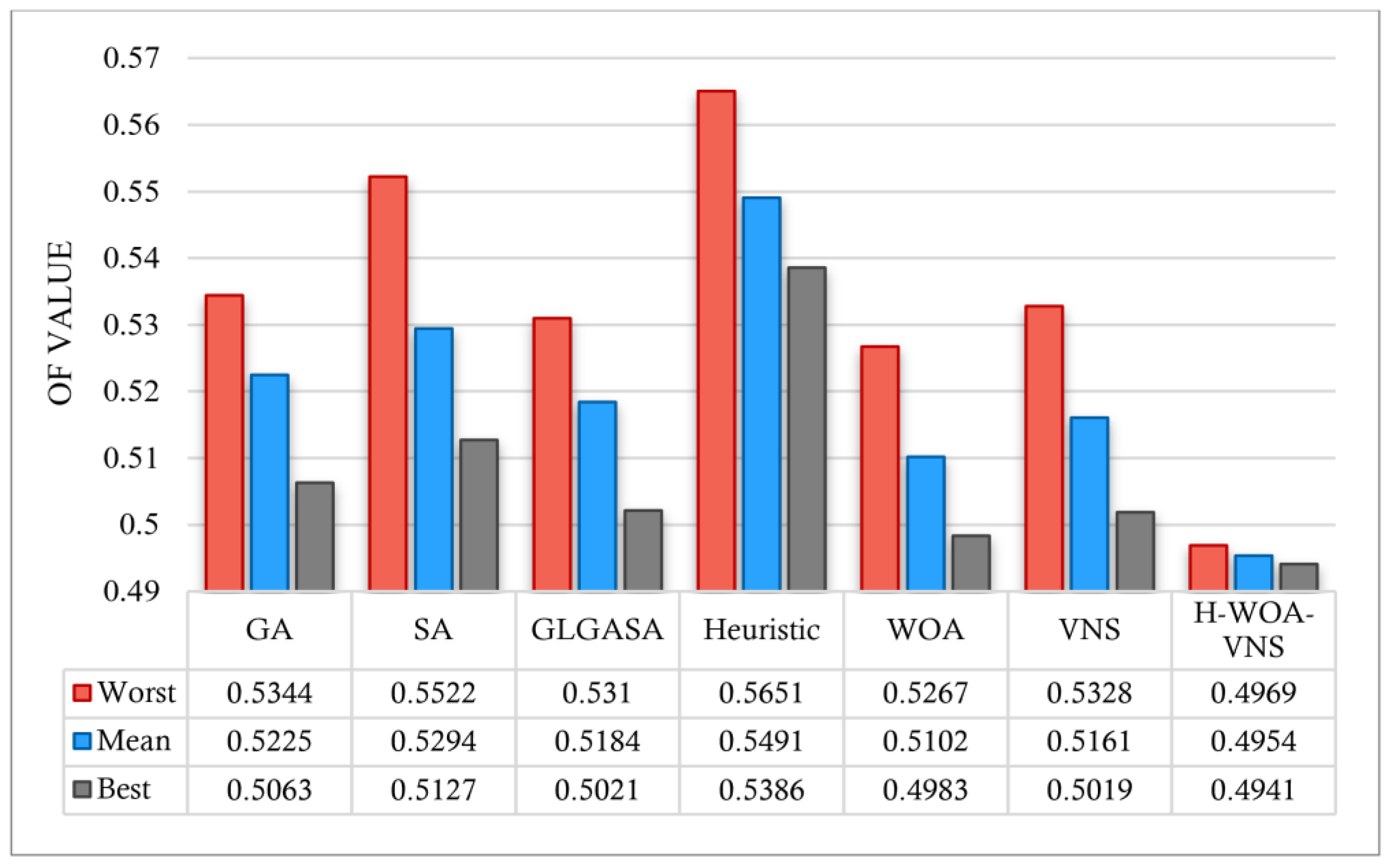
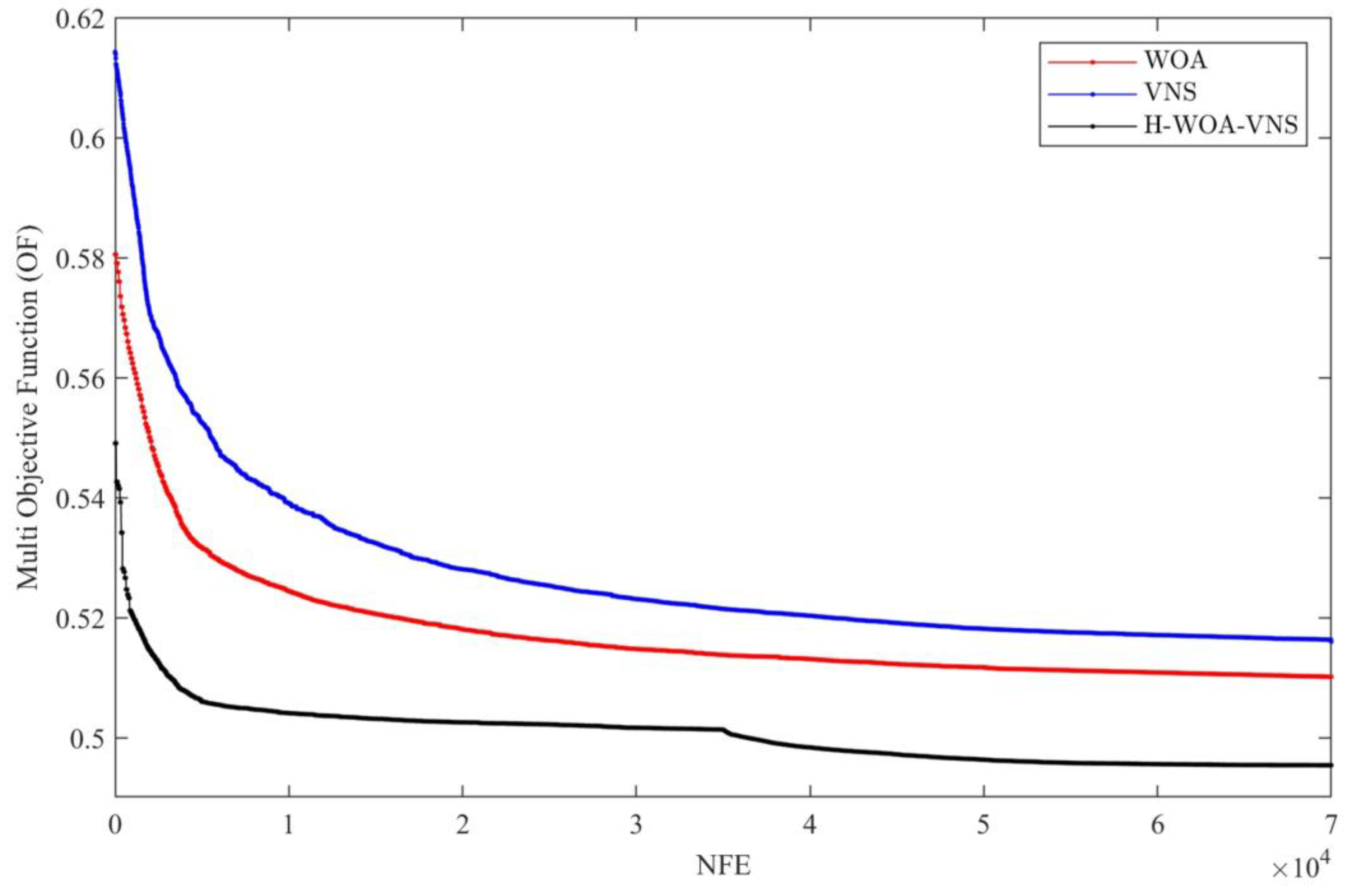
| Run | Heuristic (Stage 1) | WOA (Stage 2) | VNS (Stage 3) | GA [45] | SA [46] | GLGASA [39] | H-WOA-VNS (Proposed) |
|---|---|---|---|---|---|---|---|
| 1 | 0.5495 | 0.5034 | 0.5283 | 0.5225 | 0.5127 | 0.5163 | 0.4961 |
| 2 | 0.5463 | 0.5267 | 0.5036 | 0.5344 | 0.5522 | 0.5222 | 0.4969 |
| 3 | 0.5571 | 0.502 | 0.5328 | 0.5107 | 0.5241 | 0.5213 | 0.4957 |
| 4 | 0.5412 | 0.5204 | 0.5078 | 0.5063 | 0.5245 | 0.5097 | 0.4941 |
| 5 | 0.5534 | 0.5156 | 0.5275 | 0.5263 | 0.5322 | 0.531 | 0.495 |
| 6 | 0.5651 | 0.4983 | 0.5224 | 0.5185 | 0.5167 | 0.5221 | 0.4954 |
| 7 | 0.5386 | 0.5066 | 0.5045 | 0.5122 | 0.542 | 0.5236 | 0.4947 |
| 8 | 0.5438 | 0.513 | 0.521 | 0.5332 | 0.5333 | 0.5021 | 0.4966 |
| 9 | 0.5444 | 0.5078 | 0.5019 | 0.5327 | 0.5191 | 0.5111 | 0.4951 |
| 10 | 0.5512 | 0.5083 | 0.5117 | 0.5278 | 0.5373 | 0.525 | 0.4944 |
| Worst | 0.5651 | 0.5267 | 0.5328 | 0.5344 | 0.5522 | 0.531 | 0.4969 |
| Best | 0.5386 | 0.4983 | 0.5019 | 0.5063 | 0.5127 | 0.5021 | 0.4941 |
| Mean | 0.5491 | 0.5102 | 0.5161 | 0.5225 | 0.5294 | 0.5184 | 0.4954 |
| STD% | 1.45 | 1.72 | 2.24 | 1.94 | 2.33 | 1.66 | 0.19 |
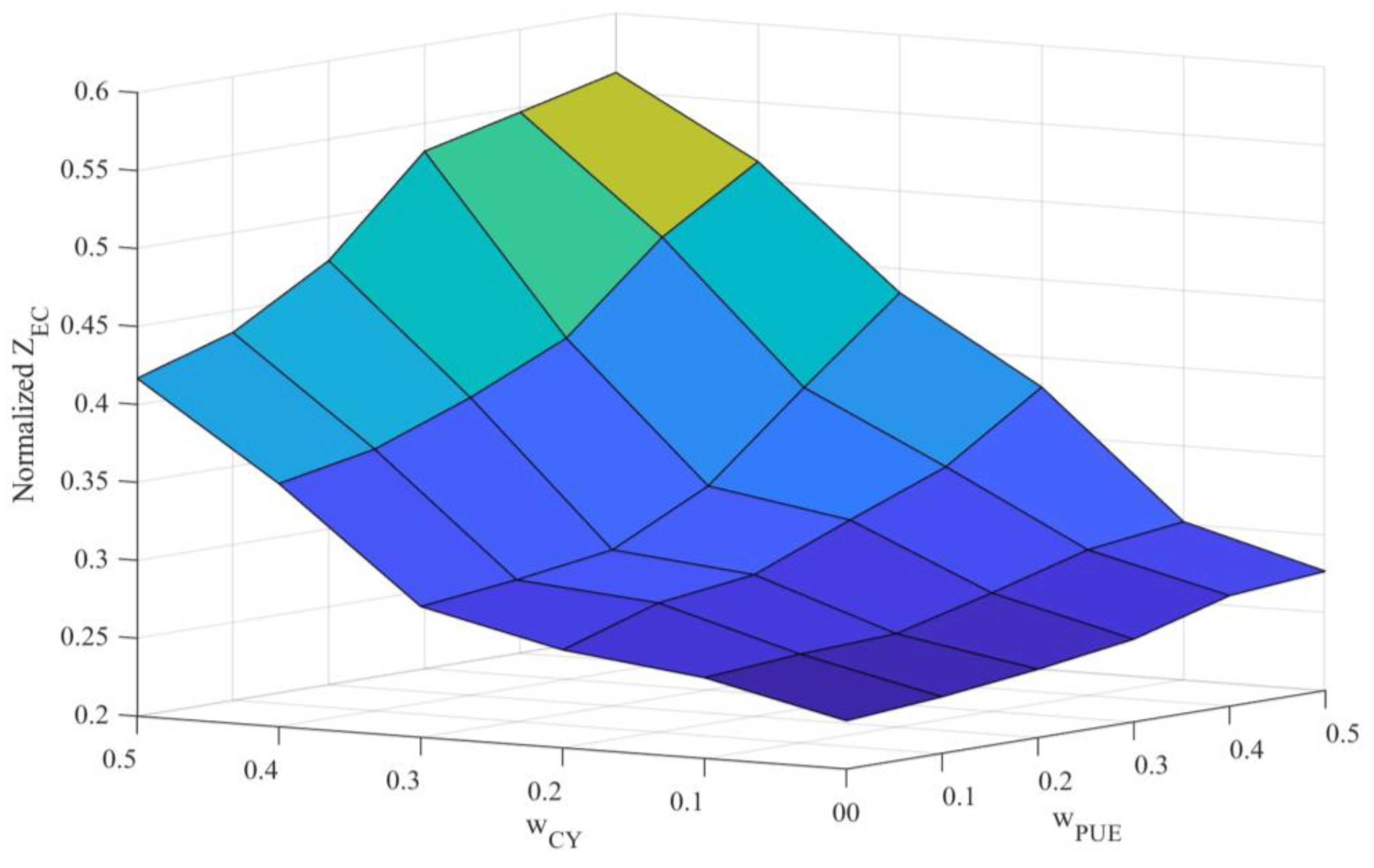
| 0.5 | 0.3 | 0.2 | 0.3001 | 0.3301 | 0.2781 |
| 0.3 | 0.5 | 0.2 | 0.472 | 0.5644 | 0.2846 |
| 0.2 | 0.3 | 0.5 | 0.4346 | 0.4032 | 0.4328 |
| 0.5 | 0.5 | 0 | 0.4167 | 0.475 | 0.2153 |
| 0.5 | 0 | 0.5 | 0.2765 | 0.2387 | 0.585 |
| 0 | 0.5 | 0.5 | 0.5623 | 0.671 | 0.5012 |
| Measure | GA | SA | GLGASA | Heuristic | WOA | VNS |
|---|---|---|---|---|---|---|
| Worst | 7.02 | 10.01 | 6.42 | 12.07 | 5.66 | 6.74 |
| Best | 2.41 | 3.63 | 1.59 | 8.26 | 0.84 | 1.55 |
| Mean | 5.19 | 6.42 | 4.44 | 9.78 | 2.9 | 4.01 |
| STD% | 90.21 | 91.85 | 88.55 | 86.9 | 88.95 | 91.52 |
Disclaimer/Publisher’s Note: The statements, opinions and data contained in all publications are solely those of the individual author(s) and contributor(s) and not of MDPI and/or the editor(s). MDPI and/or the editor(s) disclaim responsibility for any injury to people or property resulting from any ideas, methods, instructions or products referred to in the content. |
© 2023 by the authors. Licensee MDPI, Basel, Switzerland. This article is an open access article distributed under the terms and conditions of the Creative Commons Attribution (CC BY) license (https://creativecommons.org/licenses/by/4.0/).
Share and Cite
Shokouhifar, M.; Sohrabi, M.; Rabbani, M.; Molana, S.M.H.; Werner, F. Sustainable Phosphorus Fertilizer Supply Chain Management to Improve Crop Yield and P Use Efficiency Using an Ensemble Heuristic–Metaheuristic Optimization Algorithm. Agronomy 2023, 13, 565. https://doi.org/10.3390/agronomy13020565
Shokouhifar M, Sohrabi M, Rabbani M, Molana SMH, Werner F. Sustainable Phosphorus Fertilizer Supply Chain Management to Improve Crop Yield and P Use Efficiency Using an Ensemble Heuristic–Metaheuristic Optimization Algorithm. Agronomy. 2023; 13(2):565. https://doi.org/10.3390/agronomy13020565
Chicago/Turabian StyleShokouhifar, Mohammad, Mahnaz Sohrabi, Motahareh Rabbani, Seyyed Mohammad Hadji Molana, and Frank Werner. 2023. "Sustainable Phosphorus Fertilizer Supply Chain Management to Improve Crop Yield and P Use Efficiency Using an Ensemble Heuristic–Metaheuristic Optimization Algorithm" Agronomy 13, no. 2: 565. https://doi.org/10.3390/agronomy13020565
APA StyleShokouhifar, M., Sohrabi, M., Rabbani, M., Molana, S. M. H., & Werner, F. (2023). Sustainable Phosphorus Fertilizer Supply Chain Management to Improve Crop Yield and P Use Efficiency Using an Ensemble Heuristic–Metaheuristic Optimization Algorithm. Agronomy, 13(2), 565. https://doi.org/10.3390/agronomy13020565