Rice Leaf Chlorophyll Content Estimation Using UAV-Based Spectral Images in Different Regions

Abstract

Estimation of crop biophysical and biochemical characteristics is the key element for crop growth monitoring with remote sensing. With the application of unmanned aerial vehicles (UAV) as a remote sensing platform worldwide, it has become important to develop general estimation models, which can interpret remote sensing data of crops by different sensors and in different agroclimatic regions into comprehensible agronomy parameters. Leaf chlorophyll content (LCC), which can be measured as a soil plant analysis development (SPAD) value using a SPAD-502 Chlorophyll Meter, is one of the important parameters that are closely related to plant production. This study compared the estimation of rice (Oryza sativa L.) LCC in two different regions (Ningxia and Shanghai) using UAV-based spectral images. For Ningxia, images of rice plots with different nitrogen and biochar application rates were acquired by a 125-band hyperspectral camera from 2016 to 2017, and a total of 180 samples of rice LCC were recorded. For Shanghai, images of rice plots with different nitrogen application rates, straw returning, and crop rotation systems were acquired by a 5-band multispectral camera from 2017 to 2018, and a total of 228 samples of rice LCC were recorded. The spectral features of LCC in each study area were analyzed and the results showed that the rice LCC in both regions had significant correlations with the reflectance at the green, red, and red-edge bands and 8 vegetation indices such as the normalized difference vegetation index (NDVI). The estimation models of LCC were built using the partial least squares regression (PLSR), support vector regression (SVR), and artificial neural network (ANN) methods. The PLSR models tended to be more stable and accurate than the SVR and ANN models when applied in different regions with R² values higher than 0.7 through different validations. The results demonstrated that the rice canopy LCC in different regions, cultivars, and different types of sensor-based data shared similar spectral features and could be estimated by general models. The general models can be implied to a wider geographic extent to accurately quantify rice LCC, which is helpful for growth assessment and production forecasts.

1. Introduction

Remote sensing (RS) with unmanned aerial vehicles (UAV) has been widely used in crop growth monitoring in the last decade due to its high time and spatial resolution [1,2,3]. The UAV platform is capable of carrying various types of sensors to acquire multi-source RS data. Red, green, and blue (RGB), multispectral, and hyperspectral cameras have been mounted on UAVs to detect agronomic traits, such as chlorophyll content [4,5,6], leaf area index [4,7,8,9,10], aboveground biomass [10,11], and nitrogen content [12,13,14], by researchers around the world.

Spectral cameras can obtain both spectra (usually in the range of visible to near infrared) and images of targets. Strictly calibrated spectra are closely related to plant biophysical and biochemical characteristics [3], which makes spectral cameras very suitable for crop growth monitoring. There are a variety of types of UAV-based spectral cameras, which are usually classified as hyperspectral and multispectral cameras and generate different kinds of data. Hyperspectral cameras have high spectral resolution (usually between 1–10 nm) with hundreds of bands and contain rich information, which is very useful for multiple crop characteristic estimations [15]. But hyperspectral image data are also large in size and difficult to deal with. In contrast to hyperspectral cameras, multispectral cameras usually have several or dozens of bands and are easier to obtain, deploy, and analyze. It has been found that the performances of different multispectral sensors (such as Mini-MCA6, Micasense RedEdge, Parrot Sequoia, and DJI P4M) and hyperspectral sensors (such as Senop HSC-2, Cubert UHD185, and OXI VNIR-40) in the same study area matched well with the field spectrometer measurements on the ground, and the correlation coefficients of spectral reflectance and several frequently-used vegetation indices for the same targets between different sensors in the same conditions usually reach 0.9 or higher, indicating good consistency [1,16,17,18,19,20,21,22]. However, the performance of hyperspectral and multispectral cameras for monitoring the characteristics of the same crop in different conditions still remains unknown.

The measurement area of UAVs, especially multi-rotor UAVs, is relatively small because of the limited flight height and battery capacity [23]. Consequentially, studies on crop monitoring with UAV-based remote sensing were always restricted to a certain limited geographic region with an area of several hectares. Therefore, questions remain about whether the spectral responses to the same trait, for example leaf chlorophyll content (LCC), are consistent on different UAV-based spectral images and in different regions, and whether the trait can be predicted by a general model.

LCC, which is closely related to plant production, is one of the most important agronomy parameters in crop growth monitoring with remote sensing [24,25]. The SPAD value, a dimensionless quantity, is the reading of the SPAD chlorophyll meter (Minolta corporation, Ltd., Osaka, Japan) that is used to measure the relative chlorophyll content of leaves [26,27]. LCC have been proved to be proportional to the amount of chlorophyll and nitrogen in the crop leaf and widely used by researchers and farmers to determine chlorophyll content and fertilizer management [28,29,30]. The greatest advantage of the SPAD chlorophyll meter is that it can nondestructively measure in situ leaf chlorophyll content in real time, which makes it ideal for the correspondence with UAV measurements. However, ground measurements using handheld SPAD chlorophyll meters can only provide the LCC of crops within a limited part of the field.

UAV-based remote sensing retrieval of LCC helps to draw the distribution map of LCC in a large-scale field investigation and has been studied by various academic groups on different crops using different sensors such as multispectral cameras, hyperspectral imagers, and RGB cameras. Spectral reflectance at green, red, red-edge, and near-infrared bands and vegetation indices such as normalized difference vegetation index (NDVI), difference vegetation index (DVI), ratio vegetation index (RVI), green normalized difference vegetation index (GNDVI), MERIS terrestrial chlorophyll index (MTCI), and excess green index (ExG) were used to build LCC estimation models for wheat, maize, and barley via different regression methods like multiple linear regression (MLR), partial least squares regression (PLSR), support vector regression (SVR), random forest regression (RFR), and back propagation neural network (BP-NN). Most of the models achieved high accuracy [1,24,31,32,33,34]. However, as far as we are aware, there is a lack of studies on the estimation of rice (Oryza sativa L.) LCC using UAV-based remote sensing in different regions and by different sensors.

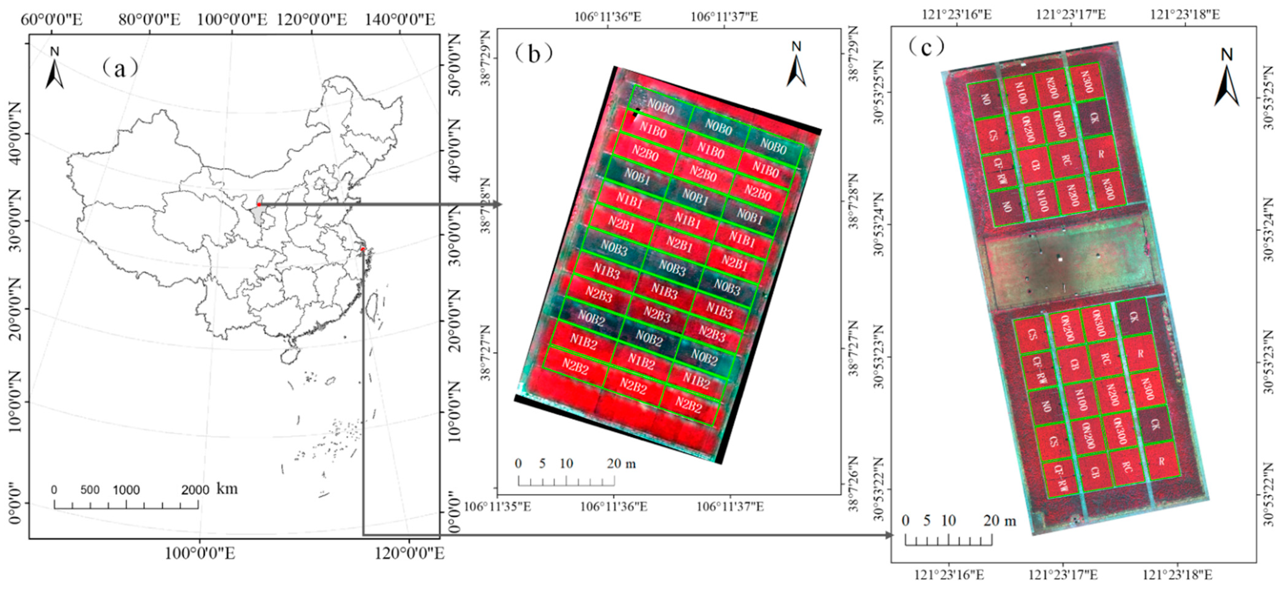
Rice, as an important food crop, is widely grown all over the world. Efficient monitoring of LCC plays an important role in the cultivation and management of rice. In this paper, the estimation of rice LCC using UAV hyperspectral and multispectral images in Ningxia and Shanghai, China, was studied to (1) investigate the spectral response characteristics of rice LCC in different geographic regions and by different sensors, and (2) establish general estimation models of rice LCC for different geographic regions and sensors.

2. Materials and Methods

2.1. Field Design and Plant Material

The field experiments were conducted in Yesheng, Qingtongxia, Ningxia (38°07′28″ N, 106°11′37″ E) and Zhuanghang, Fengxian District, Shanghai (30°33′25″ N, 121°23′17″ E), China, respectively (Figure 1a).

Yesheng, Ningxia has a temperate arid climate, which is denoted by BSk in the Köppen climate classification system. The average annual temperature is about 8.5 °C, the annual precipitation is about 220 mm, and the annual sunshine hours are between 2800 to 3000 h. The landform type is the Yellow River alluvial plain, and the soil type is anthropogenic alluvial soil. The Yellow River water is introduced for irrigation. The land is fertile and suitable for rice growth. The rice variety planted in the experimental field of Ningxia was Ningjing No.37. The rice was grown under three nitrogen (N) regimes in combination with 4 biochar (B) levels. Nitrogen regimes were: (i) 0 kg ha⁻¹ (N0), (ii) 240 kg ha⁻¹ (N1), and (iii) 300 kg ha⁻¹ (N2). Biochar levels were: (i) 0 kg ha⁻¹ (B0), (ii) 4500 kg ha⁻¹ (B1), (iii) 9000 kg ha⁻¹ (B2), and (iv) 13,500 kg ha⁻¹ (B3). The phosphate and potash fertilizers, which were applied equally to all plots were P₂O₅ (90 kg ha⁻¹) and K₂O (90 kg ha⁻¹), respectively. Treatments were arranged in a split-plot experimental design with three replicates. The size of each plot was 14 m × 5 m.

Zhuanghang, Shanghai is located in the alluvial plain of the Yangtze River Delta with a flat terrain and intersecting river networks and has a subtropical marine monsoon climate (Cfa in Köppen-Geiger classification). The average annual temperature is about 15.8 °C, the annual precipitation is about 1221 mm, and the annual sunshine hours is about 1920 h. The soil type is paddy soil. These climatic and soil conditions make it a traditional rice-growing area. The rice variety planted in the experimental field in Shanghai was Huhan No.61. There were 36 split plots. The size of each plot was 7 m × 8 m. Three different experiments were designed in these plots. For 18 plots, 6 N fertilizer treatments were set up with 3 replicates as follows: (i) no N fertilizer (N0), chemical N fertilizer at the rate of (ii) 100 kg ha⁻¹ (N100), (iii) 200 kg ha⁻¹ (N200), (iv) 300 kg ha⁻¹ (N300), and combinations of chemical and organic N fertilizers at the rates of (v) 200 kg ha⁻¹ (ON200), and (vi) 300 kg ha⁻¹ (ON300). For the other 12 plots, treatments were performed in triplicate as follows: (i) no fertilizer application (CK), (ii) conventional inorganic fertilizer application with 200 kg N ha ⁻¹(CF), (iii) the same total pure nitrogen application as in CF plus 3000 kg ha⁻¹ straw returning to the field (CS), and (iv) the same total pure nitrogen application as in CF plus 1000 kg ha⁻¹ straw-derived biochar returning to the field (CB). For the rest 6 plots and 3 CF plots, 3 different crop rotation systems were applied with 3 replicates: (i) single rice rotation (R), (ii) rice-Chinese milk vetch rotation (RC), and (iii) rice-winter wheat rotation (RW), which were applied in 3 CF plots, and 200 kg N ha⁻¹ were applied to the rice. The definitions of acronyms used here are listed in

Table 1. Definition of acronyms used in the experimental design in Shanghai.

Acronym	Definition
N	Nitrogen
ON	combinations of chemical and organic N fertilizers
CK	no fertilizer application
CF	conventional inorganic fertilizer
CS	conventional inorganic fertilizer plus straw returning
CB	conventional inorganic fertilizer plus straw-derived biochar returning
R	rice
RC	rice-Chinese milk vetch rotation
RW	rice-winter wheat rotation

.

2.2. Field Data Acquisition and Processing

2.2.1. Spectral Image Acquisition and Processing

The hyperspectral images of the rice canopy were captured in Ningxia. The sensor used here was a Cubert S185 hyperspectral imager (Cubert GmbH, Ulm, Germany) mounted on an octocopter UAV. The spectral range of S185 is 450–950 nm with 125 bands, and the spectral sampling interval is 4 nm. It acquires a hyperspectral image with 50 by 50 pixels for each band. The flight height was 70 m, resulting in a spatial resolution of 0.53 m. The forward and side overlaps were set at 85% and 80%, respectively. One frame of hyperspectral image was captured every second for about 12 min in each flight mission. Five flight missions were conducted in the rice field at different growth stages on 19 July 2016, 16 August 2016, 9 July 2017, 10 August 2017 and 11 September 2017. All flight missions were performed between 11:00 and 13:00 in cloudless weather.

The multispectral images of the rice canopy were captured in Shanghai. The sensor used here was a Micasense RedEdge 3 multispectral camera (Micasense Inc., Seattle, WA, USA) mounted on a DJI M600 Pro UAV (SZ DJI Technology Co., Shenzhen, China). RedEdge 3 acquires five-band images with 1280 by 960 pixels at five discrete wavelength ranges: blue (475 ± 20 nm), green (560 ± 20 nm), red (668 ± 20 nm), red-edge (−717 ± 10 nm), and near infrared (NIR) (840 ± 40 nm). The flight height was 100 m, yielding a spatial resolution of 0.06 m. The forward and side overlaps were set at 85% and 80%, respectively. One multispectral image was captured every second for about 15 min in each flight mission. Eight flight missions were conducted in the rice field at different growth stages on 4 August 2017, 11 August 2017, 8 September 2017, 10 October 2017, 19 July 2018, 23 August 2018, 29 September 2018, and 15 October 2018. All flight missions were performed between 11:00 and 13:00 in cloudless weather.

Spectral images were radiometrically calibrated according to the reflectance of the reference panels on the ground. The reference panel of S185 (Cubert GmbH, Ulm, Germany) is a white board with 100% reflectance by the size of 50 cm × 50 cm. The reference panel of RedEdge 3 (Micasense Inc., Seattle, WA, USA) is a gray board with 50% reflectance and a size of 15.5 cm × 15.5 cm. The hyperspectral images of the whole rice field in Ningxia were generated by mosaicking the images within the aerial survey area using Agisoft PhotoScan Professional (Agisoft LLC, St. Petersburg, Russia). The multispectral image of the whole rice field in Shanghai was generated by mosaicking the images within the aerial survey area using Pix4DmapperPro (PIX4D, Lausanne, Switzerland). Geometric correction and projection transformation were applied to the mosaicked image according to the ground control points (GCPs) using ArcGIS (ESRI, Redlands, CA, USA), as shown in Figure 1b,c. The number of GCPs was eight in Ningxia and ten in Shanghai. The plot boundaries were drawn according to the images in ArcGIS and buffered by 0.5 m to create the plot boundary files for spectra extraction. The mean spectra of all pixels inside the buffered plot boundary were calculated for each plot using ENVI 5.6 software (Harris Geospatial Solutions, Inc., Broomfield, CO, America).

Vegetation indices are usually calculated by linear or nonlinear combination of reflectance data at different bands and designed to maximize sensitivity to the vegetation characteristics while minimizing confounding factors such as soil background reflectance, directional, or atmospheric effects, which will cause fluctuation and noise in reflectance [35,36]. In this study, we tested dozens of broad-band vegetation indices that were commonly used for LCC estimation. Eight of them, which are applicable for both the hyperspectral imager (S185) and multispectral camera (RedEdge 3), were selected for this study (

Table 2. Vegetation indices used in this study.

Vegetation Index	Acronym	Equation	Reference
Normalized difference vegetation index	NDVI	(R840 − R668)/(R840 + R668)	[37]
Ratio vegetation index	RVI	R840/R668	[38]
Green normalized difference vegetation index	GNDVI	(R840 − R560)/(R840 + R560)	[39]
Green ratio vegetation index	GRVI	R840/R560	[40]
Red-edge normalized difference vegetation index	RENDVI	(R840 − R717)/(R840 + R717)	[41]
Red-edge ratio vegetation index	RERVI	R840/R717	[40]
Normalized pigment/chlorophyll index	NPCI	(R668 − R475)/(R668 + R475)	[42]
MERIS terrestrial chlorophyll index	MTCI	(R840 − R717)/(R717 − R668)	[43]

R represents the reflectance value in specified bands.

). In the calculation of vegetation indices for the hyperspectral images by S185, we chose the spectral reflectance at the wavelength of 475 nm for the blue band, 560 nm for the green band, 668 nm for the red band, 717 nm for the red-edge band, and 840 nm for the NIR band.

2.2.2. Rice LCC Measurement

Twenty flag leaves of rice away from the edge were selected randomly in each plot for LCC measurment by the SPAD-502 (Minolta Camera Co., Osaka, Japan) right after the flight mission on the day of every UAV survey. The average SPAD value of the 20 leaves was calculated as the LCC of a given plot, and the SPAD value of each plot was recorded as a sample. Finally, a total of 180 samples in Ningxia and 228 samples in Shanghai were recorded.

2.3. Statistical Analysis

2.3.1. Correlational Analysis

Correlational analysis was employed to investigate the response of spectral reflectance and vegetation indices to rice LCC. The Pearson’s correlation coefficients (r) between LCC and the spectral parameters (reflectance and vegetation indices) in Ningxia and Shanghai was calculated using Equation (1):

$$r=\frac{{\sum }_{i=1}^n\left(x_i-\overline{x}\right)\left(y_i-\overline{y}\right)}{\sqrt{{\sum }_{i=1}^n{\left(x_i-\overline{x}\right)}^2}\sqrt{{\sum }_{i=1}^n{\left(y_i-\overline{y}\right)}^2}}$$

(1)

where n is the sample size, x_i and y_i are the individual sample i, $\overline{x_i}$ is the mean value of all x samples, and analogously for $\overline{y_i}$. An absolute value of r closer to 1 indicates a better correlation between x and y.

2.3.2. Regression Analysis

Three groups of datasets were established from the collected data: Ningxia, Shanghai, and Ningxia-Shanghai. The Ningxia group contained 180 samples. The Shanghai group contained 228 samples. The Ningxia-Shanghai group, which was the combination of the Ningxia and Shanghai groups, contained 408 samples. Each dataset was split into two parts of sub-datasets, with 2/3 for model calibration (Cal) and the rest, 1/3 for validation (Val). The Ningxia-Shanghai calibration (Ningxia-Shanghai_Cal, 272 samples) sub-dataset consisted of the Ningxia calibration (Ningxia_Cal, 120 samples) and Shanghai calibration (Shanghai_Cal, 152 samples) sub-datasets. The Ningxia-Shanghai validation (Ningxia-Shanghai_Val, 136 samples) sub-dataset consisted of the Ningxia validation (Ningxia_Val, 60 samples) and Shanghai validation (Shanghai_Val, 76 samples) sub-datasets.

For each of the three groups of datasets, rice LCC estimation models were established by taking the vegetation indices as independent variables and using three methods: PLSR, SVR, and Artificial Neural Network (ANN). PLSR is a multiple linear regression method integrating principal component analysis, correlation analysis, and canonical correlation analysis. PLSR helps to build stable models by effectively eliminating multiple correlations between the independent variables and extracting the composite variables, which are most explanatory of the dependent variables [44,45,46,47]. SVR is a machine-learning regression algorithm based on statistical learning theory. By using kernel functions, the input data is mapped into a higher-dimensional space, in which the optimal regression models are constructed [48]. ANN is a nonlinear machine learning algorithm that mimics the structure and function of biological neural networks [49].

In this study, the number of components for the PLSR model was determined when the overall mean predicted R², calculated based on the predicted residual sum of squares (PRESS) reached a maximum in the LeaveOne-Out Cross Validation (LOOCV) scheme. For SVR models, the Gaussian function was adopted as the kernel, and the grid search method and cross validation were used to determine the parameters. For ANN models, the multilayer feedforward neural network (including the input layer, hidden layer, and output layer) was used to build the SPAD estimation models, and the training algorithm was chosen as Levenberg-Marquardt and the hidden layer number was set as 5.

The coefficient of determination (R²), root mean square error (RMSE), and mean absolute percentage error (MAPE) were used to evaluate the predictive performance of each model. The equations of R², RMSE, and MRE are presented in Equations (2)–(4):

$${\mathrm{R}}^2=1-\frac{{\sum }_{i=1}^n(y_i-\widehat{y_i}{)}^2}{{\sum }_{i=1}^n(y_i-\overline{y_i}{)}^2}$$

(2)

$$\mathrm{RMSE}=\sqrt{\frac{{\sum }_{i=1}^n(y_i-\widehat{y_i}{)}^2}{n}}$$

(3)

$$\mathrm{MAPE}=\frac{100}{n}\sum _{i=1}^n\left|\frac{y_i-\widehat{y_i}}{y_i}\right|$$

(4)

where n is the number of samples, y_i and $\widehat{y_i}$ is the measured and predicted value of sample i, $\overline{y_i}$ is the average value of all samples. A higher R² value (close to 1) with a lower RMSE and MAPE (close to 0) indicate a better model accuracy.

Two kinds of validation were applied to test the prediction accuracy and generalization ability of the different models. First, the models were validated within the groups in which they were built. Second, the models were validated interactively, that is to say, validating the models built based on the Ningxia (Shanghai) group using data from the Shanghai (Ningxia) group, by which the most stable modelling method could be revealed. All these statistical analyses were performed using the MATLAB R2018a software (MathWorks, Natick, MA, USA).

3. Results

3.1. Statistics of LCC

Table 3. Statistical characteristics of rice LCC in Ningxia and Shanghai.

Study Area	Sample Number	Maximum	Minimum	Mean	Median	Standard Deviation
Ningxia	180	49.4	12.5	34.8	37.6	8.9
Shanghai	228	48.6	15.7	39.1	40.7	6.2

shows the summary statistics for the measured LCC of rice leaves in Ningxia and Shanghai. The statistical characteristics of rice LCC showed similar tendencies in these two study areas.

3.2. Response of Spectral Reflectance and Vegetation Indices to Rice LCC

The correlation between the spectral reflectance at each band and rice LCC in Ningxia and Shanghai showed a similar pattern in the wavelength range of 450–720 nm with significant negative correlations (|r| > 0.4), as shown in Figure 2. The highest correlations appeared in the red bands in both Ningxia and Shanghai, with r = −0.88 at 670 nm for Ningxia and r = −0.80 at 668 nm for Shanghai. At the NIR range, the correlations between spectral reflectance and LCC were slightly positive for the rice in Ningxia and significantly positive for the rice in Shanghai with r = 0.44.

As shown in

Table 4. Correlation coefficients between vegetation indices and rice LCC in Ningxia and Shanghai.

Vegetation Index	Correlation Coefficient
	Ningxia	Shanghai
NDVI	0.75 **	0.85 **
RVI	0.67 **	0.78 **
GNDVI	0.61 **	0.78 **
GRVI	0.59 **	0.75 **
RENDVI	0.64 **	0.84 **
RERVI	0.58 **	0.82 **
NPCI	−0.81 **	−0.71 **
MTCI	0.47 **	0.79 **

** denotes significant correlation at the 0.01 level.

, all of the eight vegetation indices were significantly correlated with rice LCC with an absolute r value higher than 0.4 in both Ningxia and Shanghai. NPCI had a high negative correlation with LCC. The other seven vegetation indices had positive correlations with LCC. NDVI and NPCI both responded to LCC better than the other vegetation indices in Ningxia with an r value of 0.75 and −0.81, respectively. The r values of RVI, GNDVI, and RENDVI were between 0.6 and 0.7, while those of GRVI, REVI, and MTCI were below 0.6. For rice in Shanghai, the r values were all above 0.7, which indicated a good response of all of the vegetation indices to LCC.

3.3. Estimation Models of Rice LCC

Estimation models of rice LCC were constructed based on the calibration sub-datasets using PLSR, SVR, and ANN methods for Ningxia, Shanghai, and Ningxia-Shanghai, respectively. As shown in

Table 5. Performance of rice LCC estimation models for Ningxia, Shanghai, and Ningxia-Shanghai combination calibration datasets based on all the eight vegetation indices.

Calibration Dataset	Method	R2	RMSE	MAPE (%)
Ningxia_Cal	PLSR	0.84	3.41	8.91
	SVR	0.89	2.88	8.40
	ANN	0.90	2.84	8.27
Shanghai_Cal	PLSR	0.82	2.14	5.36
	SVR	0.90	1.63	4.13
	ANN	0.88	1.76	4.48
Ningxia-Shanghai_Cal	PLSR	0.81	3.33	8.9
	SVR	0.88	2.57	6.91
	ANN	0.89	2.47	6.66

, all models yielded good performances, with R² values higher than 0.8, RMSE lower than 3.5, and MAPE lower than 10%. The models of the Shanghai group performed better than those of the Ningxia and Ningxia-Shanghai groups, with RMSE values lower than 2.2 and a MAPE below 5.4%. The models of Ningxia, in which the RMSE was higher than 2.8 and MAPE was above 8.2%, were less accurate compared with the other two groups. The performances of Ningxia-Shanghai models were at moderate levels. Two machine learning methods, SVR and ANN, were superior to PLSR, with an R² value between 0.88 and 0.90 and a smaller RMSE and MAPE.

3.4. Validation of Rice LCC Estimation Models

3.4.1. Validation of Models within the Group

Validation sub-datasets for each group were used to evaluate the prediction accuracy of the LCC estimation models for their group. As shown in

Table 6. Validation of rice leaf LCC estimation models for the same group.

Validation Dataset	Model	R2	RMSE	MAPE (%)
Ningxia_Val	Ningxia_PLSR	0.81	4.00	11.87
	Ningxia_SVR	0.86	3.48	10.23
	Ningxia_ANN	0.86	3.45	10.15
Shanghai_Val	Shanghai_PLSR	0.79	2.24	5.72
	Shanghai_SVR	0.86	2.00	5.11
	Shanghai_ANN	0.84	2.08	5.31
Ningxia-Shanghai_Val	Ningxia-Shanghai_PLSR	0.76	3.69	10.03
	Ningxia-Shanghai_SVR	0.84	2.93	7.94
	Ningxia-Shanghai_ANN	0.84	3.01	8.11

and Figure 3, the models for Shanghai yielded the highest prediction accuracy, with an RMSE between 2.08 and 2.24 and MAPE between 5.11% to 5.72%. The models of Ningxia turned out to be lower in prediction accuracy, with an RMSE between 3.45 and 4.00 and MAPE larger than 10.1%. In terms of modeling methods, SVR and ANN models had better predictive ability than the PLSR model in each group, with an R² value between 0.84 and 0.86 and lower values of RMSE and MAPE. Scatter plots between measured and predicted LCC along the 1:1 line indicated a trend that lower LCC were overestimated by all the models in the Ningxia and Ningxia-Shanghai groups (Figure 3).

3.4.2. Interactive Validation of Models

In order to test whether the UAV-based rice LCC estimation models built in one study area could be used in another region with a different sensor, here we use all the data in the Ningxia group (Ningxia_All) to validate the rice LCC estimation models built based on the Shanghai group and all the data in the Shanghai group (Shanghai_All) to validate the models constructed based on the Ningxia group. The results are given in

Table 7. Interactive validation of rice LCC estimation models of Ningxia and Shanghai.

Validation Dataset	Model	R2	RMSE	MAPE (%)
Ningxia_All	Shanghai_PLSR	0.74	5.45	15.95
	Shanghai_SVR	0.14	15.38	45.03
	Shanghai_ANN	0.69	5.80	17.00
Shanghai_All	Ningxia_PLSR	0.71	6.21	15.84
	Ningxia_SVR	0.69	6.76	16.14
	Ningxia_ANN	0.12	13.38	34.11

and Figure 4. For both Ningxia and Shanghai, the PLSR models outperformed the SVR and ANN models in predictive accuracy and stability, with R² values of 0.74 and 0.71, RMSE values of 5.45 and 6.21, and MAPE values of 15.95% and 15.84%, respectively. The predicted rice LCC of Ningxia using the Shanghai_ANN model and those of Shanghai using the Ningxia_SVR model were less accurate, with an R² vaue of 0.69, RMSE values of 5.80 and 6.76, and MAPE values of 17.00% and 16.14%. However, as can be observed from Figure 4, the predicted rice LCCs of Ningxia using the Shanghai_SVR model and those of Shanghai using the Ningxia_ANN model greatly deviated from the measured values with very low R² values of 0.14 and 0.12, high RMSE values of 15.38 and 13.38, and large MAPE of values 45.3% and 34.11%, respectively.

4. Discussion

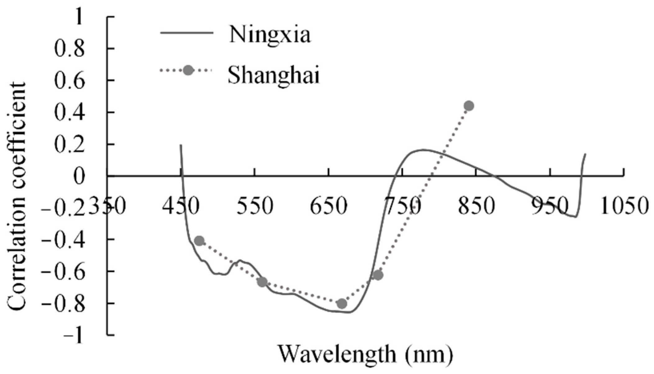
In this study, we found that despite the differencse in the region, variety, and sensor, the correlation between rice LCC, spectral reflectance, and vegetation indices in Ningxia and Shanghai had similarities. This result was in accordance with the previous findings by researchers on the spectral characteristics of rice LCC or chlorophyll content using visible and near-infrared spectrometers [50,51,52,53], which indicated that the spectral responses of rice LCC or chlorophyll content shared the same pattern, that is, the spectral reflectance and rice LCC had significant negative correlations at the wavelength range of 450–720 nm. The eight vegetation indices were found to be closely related to rice LCC, which was in accordance with the findings by Xie [50]. On the other side, differences in spectral reflectance in the NIR range between Ningxia and Shanghai can be observed. The most possible reason was that the Shanghai group contained more data collected in the maturation stage, when the correlation between LCC and spectral reflectance in the NIR range was higher than at other growth stages [54]. Similar phenomena were also found in other crops such as wheat, maize, and potatoes [25,55,56]. Since the field remote sensing data collection largely depended on weather conditions, the growth stages when the field campaigns were carried out were not unified in different study areas and years. The difference between Ningxia and Shanghai groups in growth stage also affected the response of vegetation indices and model accuracy.

Theoretically, the reflectance of the same target measured under standard conditions by different spectral sensors, which are strictly calibrated should be coincident. However, in the actual measurement operation, the spectral reflectance value is affected by band-response functions, spatial resolution, and environmental factors such as atmospheric transmissivity, solar zenith angle, solar declination angle, and soil background, which would cause a systematic difference [1,57]. Vegetation indices, which are designed to be particularly sensitive to vegetative covers, are less affected by those factors [58,59]. The rice fields in Ningxia and Shanghai are at different latitudes, with different soil backgrounds and solar illumination geometry. The spectral response functions and spatial resolution of S185 and Redege 3 also vary. In order to minimize the error in spectral reflectance caused by the environment and sensor type and make the variables available for both regions, vegetation indices rather than spectral reflectance were chosen as independent variables in the rice leaf SPAD estimation models.

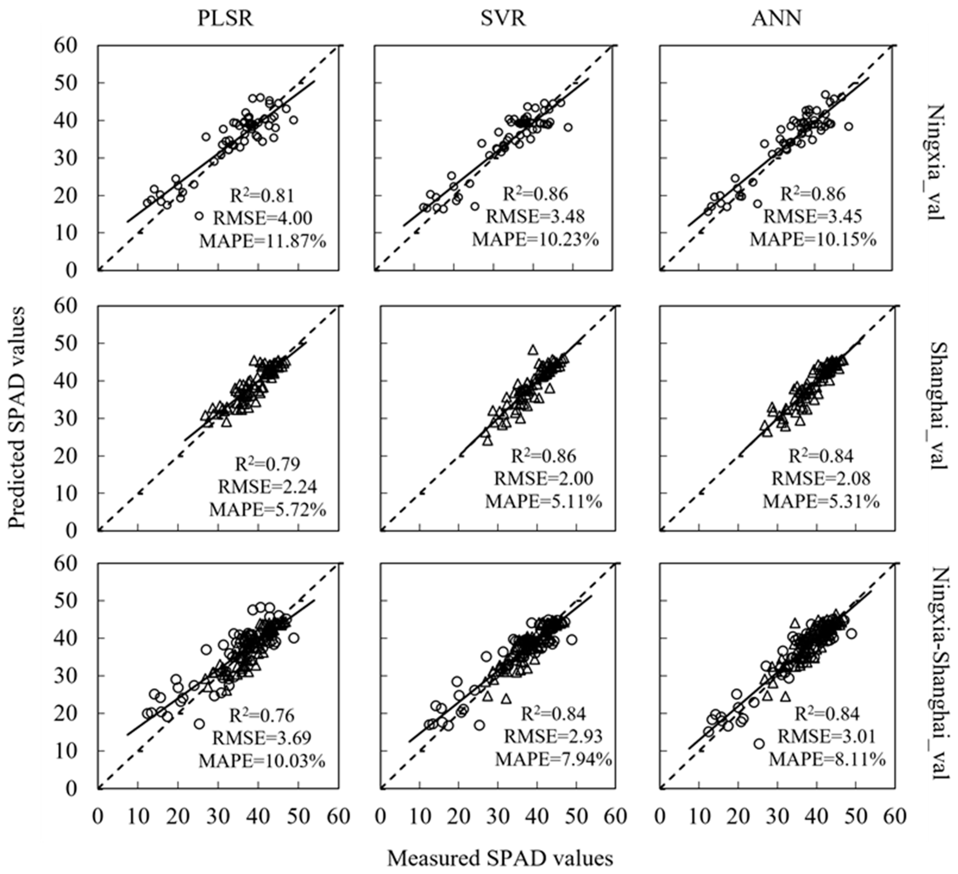
The validation of rice LCC estimation models for the Ningxia-Shanghai group indicated that the models were capable of predicting LCC of rice in both Ningxia and Shanghai with relatively low errors, which answered the question of whether a certain crop trait could be predicted by a general model for different regions and sensors. 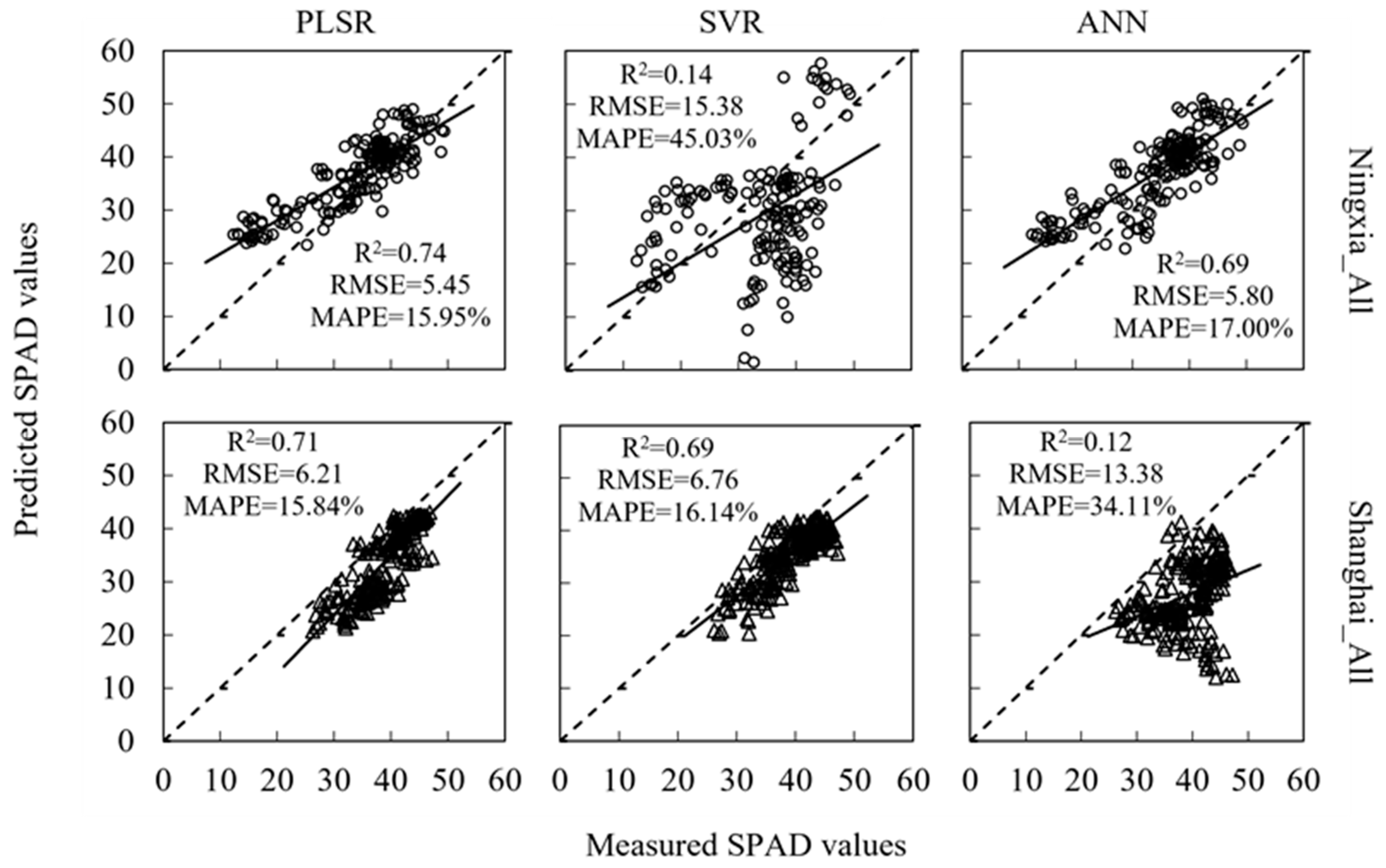In addition, the interaction validation of PLSR models of Ningxia and Shanghai in Section 3.4.2 also yielded good predicting results with MAPE less than 20%, which indicated that, based on the same spectral response pattern, a model of the same crop trait constructed for one region and spectral sensor using the PLSR method was still available for another region and sensor. It is impossible to build new models for every new region in the application of remote sensing monitoring of crop growth. In cases where no prior data is available, models transplanted from another region and sensors could be used to provide informative results.

The performances of models using different regression methods varied in validation steps. Models using two machine learning methods, SVR and ANN, achieved high accuracy when validated by the validation sub-dataset from the same group of the dataset (Section 3.4.1). However, the LCC prediction accuracy decreased dramatically when SVR or ANN models for one region were applied to the other, implying limited generalization ability (Section 3.4.2). PLSR models showed better prediction accuracy and stability in the interactive validation. Although machine learning is effective in data mining, the lack of interpretability may increase the uncertainty of the model [60]. Previous studies have suggested that the training data has a strong influence on the performance of machine learning methods, and extreme attention should be paid when applying regression models with machine learning algorithms to data collected under different conditions from the training data [61]. There are several possible explanations, as follows: The data from the two study areas had global features in common (for example, the same spectral response pattern as LCC), as well as local features of their own that were caused by the difference in location, cultivar, and sensor. Two machine learning methods, SVR and ANN, would make the most of both global and local features within the training dataset in the modeling procress to minimize prediction error. However, the difference in local features would lower the prediction accuracy when applying the machine learning-based models to another dataset. In contrast, the PLSR method mainly used global features in model construction, thus resulting in better generalization ability than SVR and ANN.

5. Conclusions

The application of UAV-based remote sensing to crop growth monitoring has gradually entered the practical stage. Therefore, it is of great importance to develop remote sensing models for crop monitoring, which are suitable for multiple regions and types of sensors. In this study, images of rice fields in two different regions were acquired by multispectral and hyperspectral cameras mounted on UAV platforms. Analysis of the spectral response of rice LCC in different regions showed a similar pattern: spectral reflectance at the green and red bands, as well as two vegetation indices (NDVI and NPCI), were highly correlated with the LCC. All the estimation models of rice LCC yielded good accuracy within the group where the training data came from. Models built with PLSR rather than SVR and ANN, which achieved outstanding performance in the interactive validation, had the potential to be used as general estimation models of rice LCC.

As far as we know, this was the first approach to building models based on UAV-based remote sensing data from different regions and sensors. It demonstrates that it is feasible to study general models for UAV-based retrieval of agronomic parameters. The outcomes of this study could be used by practitioners and organizations to develop sensors that can directly produce LCC or chlorophyll content distribution maps based on spectral images of rice fields, which is very intuitive and helpful for farmers.

This study involved two independent experiments, the conditions of which varied in many aspects. It is difficult to analyze the influence of specific factors on the LCC estimation. Therefore, this paper focused on finding the common points in the spectral response and estimation models of the two experiments. In the future, experiments with carefully controlled conditions should be designed for more in-depth studies on the influence of specific factors such as flight height, time, and weather.

References

1. Deng, L.; Mao, Z.; Li, X.; Hu, Z.; Duan, F.; Yan, Y. UAV-based multispectral remote sensing for precision agriculture: A comparison between different cameras. ISPRS J. Photogramm. Remote Sens. 2018, 146, 124–136. [Google Scholar] [CrossRef]
2. Delavarpour, N.; Koparan, C.; Nowatzki, J.; Bajwa, S.; Sun, X. A technical study on UAV characteristics for precision agriculture applications and associated practical challenges. Remote Sens. 2021, 13, 1204. [Google Scholar] [CrossRef]
3. Tsouros, D.C.; Bibi, S.; Sarigiannidis, P.G. A review on UAV-based applications for precision agriculture. Information 2019, 10, 349. [Google Scholar] [CrossRef] [Green Version]
4. Kanning, M.; Kühling, I.; Trautz, D.; Jarmer, T. High-resolution UAV-based hyperspectral imagery for LAI and chlorophyll estimations from wheat for yield prediction. Remote Sens. 2018, 10, 2000. [Google Scholar] [CrossRef] [Green Version]
5. Guo, Y.; Yin, G.; Sun, H.; Wang, H.; Chen, S.; Senthilnath, J.; Wang, J.; Fu, Y. Scaling effects on chlorophyll content estimations with RGB camera mounted on a UAV platform using machine-learning methods. Sensors 2020, 20, 5130. [Google Scholar] [CrossRef]
6. Singhal, G.; Bansod, B.; Mathew, L.; Goswami, J.; Choudhury, B.; Raju, P. Chlorophyll estimation using multi-spectral unmanned aerial system based on machine learning techniques. Remote Sens. Appl. Soc. Environ. 2019, 15, 100235. [Google Scholar] [CrossRef]
7. Li, S.; Yuan, F.; Ata-UI-Karim, S.T.; Zheng, H.; Cheng, T.; Liu, X.; Tian, Y.; Zhu, Y.; Cao, W.; Cao, Q. Combining color indices and textures of UAV-based digital imagery for rice LAI estimation. Remote Sens. 2019, 11, 1763. [Google Scholar] [CrossRef] [Green Version]
8. Qiao, L.; Gao, D.; Zhao, R.; Tang, W.; An, L.; Li, M.; Sun, H. Improving estimation of LAI dynamic by fusion of morphological and vegetation indices based on UAV imagery. Comput. Electron. Agric. 2022, 192, 106603. [Google Scholar] [CrossRef]
9. Duan, B.; Liu, Y.; Gong, Y.; Peng, Y.; Wu, X.; Zhu, R.; Fang, S. Remote estimation of rice LAI based on Fourier spectrum texture from UAV image. Plant Methods 2019, 15, 124. [Google Scholar] [CrossRef] [Green Version]
10. Tao, H.; Feng, H.; Xu, L.; Miao, M.; Long, H.; Yue, J.; Li, Z.; Yang, G.; Yang, X.; Fan, L. Estimation of crop growth parameters using UAV-based hyperspectral remote sensing data. Sensors 2020, 20, 1296. [Google Scholar] [CrossRef]
11. Yue, J.; Yang, G.; Tian, Q.; Feng, H.; Xu, K.; Zhou, C. Estimate of winter-wheat above-ground biomass based on UAV ultrahigh-ground-resolution image textures and vegetation indices. ISPRS J. Photogramm. Remote Sens. 2019, 150, 226–244. [Google Scholar] [CrossRef]
12. Näsi, R.; Viljanen, N.; Kaivosoja, J.; Alhonoja, K.; Hakala, T.; Markelin, L.; Honkavaara, E. Estimating biomass and nitrogen amount of barley and grass using UAV and aircraft based spectral and photogrammetric 3D features. Remote Sens. 2018, 10, 1082. [Google Scholar] [CrossRef] [Green Version]
13. Kefauver, S.C.; Vicente, R.; Vergara-Díaz, O.; Fernandez-Gallego, J.A.; Kerfal, S.; Lopez, A.; Melichar, J.P.; Serret Molins, M.D.; Araus, J.L. Comparative UAV and field phenotyping to assess yield and nitrogen use efficiency in hybrid and conventional barley. Front. Plant Sci. 2017, 8, 1733. [Google Scholar] [CrossRef] [PubMed]
14. Colorado, J.D.; Cera-Bornacelli, N.; Caldas, J.S.; Petro, E.; Rebolledo, M.C.; Cuellar, D.; Calderon, F.; Mondragon, I.F.; Jaramillo-Botero, A. Estimation of nitrogen in rice crops from UAV-captured images. Remote Sens. 2020, 12, 3396. [Google Scholar] [CrossRef]
15. Lu, B.; Dao, P.D.; Liu, J.; He, Y.; Shang, J. Recent advances of hyperspectral imaging technology and applications in agriculture. Remote Sens. 2020, 12, 2659. [Google Scholar] [CrossRef]
16. Bareth, G.; Aasen, H.; Bendig, J.; Gnyp, M.L.; Bolten, A.; Jung, A.; Michels, R.; Soukkamäki, J. Low-weight and UAV-based Hyperspectral Full-frame Cameras for Monitoring Crops: Spectral Comparison with Portable Spectroradiometer Measurements. In Photogrammetrie-Fernerkundung-Geoinformation; E. Schweizerbart’sche Verlagsbuchhandlung: Stuttgart, Germany, 2015; pp. 69–79. [Google Scholar]
17. Di Gennaro, S.F.; Toscano, P.; Gatti, M.; Poni, S.; Berton, A.; Matese, A. Spectral Comparison of UAV-Based Hyper and Multispectral Cameras for Precision Viticulture. Remote Sens. 2022, 14, 449. [Google Scholar] [CrossRef]
18. Von Bueren, S.K.; Burkart, A.; Hueni, A.; Rascher, U.; Tuohy, M.P.; Yule, I.J. Deploying four optical UAV-based sensors over grassland: Challenges and limitations. Biogeosciences 2015, 12, 163–175. [Google Scholar] [CrossRef] [Green Version]
19. Lu, H.; Fan, T.; Ghimire, P.; Deng, L. Experimental evaluation and consistency comparison of UAV multispectral minisensors. Remote Sens. 2020, 12, 2542. [Google Scholar] [CrossRef]
20. Crucil, G.; Castaldi, F.; Aldana-Jague, E.; van Wesemael, B.; Macdonald, A.; Van Oost, K. Assessing the performance of UAS-compatible multispectral and hyperspectral sensors for soil organic carbon prediction. Sustainability 2019, 11, 1889. [Google Scholar] [CrossRef] [Green Version]
21. Abdelbaki, A.; Schlerf, M.; Retzlaff, R.; Machwitz, M.; Verrelst, J.; Udelhoven, T. Comparison of crop trait retrieval strategies using UAV-based VNIR hyperspectral imaging. Remote Sens. 2021, 13, 1748. [Google Scholar] [CrossRef]
22. Deng, L.; Yan, Y.; Gong, H.; Duan, F.; Zhong, R. The effect of spatial resolution on radiometric and geometric performances of a UAV-mounted hyperspectral 2D imager. ISPRS J. Photogramm. Remote Sens. 2018, 144, 298–314. [Google Scholar] [CrossRef]
23. Hassler, S.C.; Baysal-Gurel, F. Unmanned aircraft system (UAS) technology and applications in agriculture. Agronomy 2019, 9, 618. [Google Scholar] [CrossRef] [Green Version]
24. Yang, X.; Yang, R.; Ye, Y.; Yuan, Z.; Wang, D.; Hua, K. Winter wheat SPAD estimation from UAV hyperspectral data using cluster-regression methods. Int. J. Appl. Earth Obs. Geoinf. 2021, 105, 102618. [Google Scholar] [CrossRef]
25. Yang, H.; Ming, B.; Nie, C.; Xue, B.; Xin, J.; Lu, X.; Xue, J.; Hou, P.; Xie, R.; Wang, K.; et al. Maize Canopy and Leaf Chlorophyll Content Assessment from Leaf Spectral Reflectance: Estimation and Uncertainty Analysis across Growth Stages and Vertical Distribution. Remote Sens. 2022, 14, 2115. [Google Scholar] [CrossRef]
26. Yamamoto, A.; Nakamura, T.; Adu-Gyamfi, J.; Saigusa, M. Relationship between chlorophyll content in leaves of sorghum and pigeonpea determined by extraction method and by chlorophyll meter (SPAD-502). J. Plant Nutr. 2002, 25, 2295–2301. [Google Scholar] [CrossRef]
27. Uddling, J.; Gelang-Alfredsson, J.; Piikki, K.; Pleijel, H. Evaluating the relationship between leaf chlorophyll concentration and SPAD-502 chlorophyll meter readings. Photosynth. Res. 2007, 91, 37–46. [Google Scholar] [CrossRef]
28. Shah, S.H.; Houborg, R.; McCabe, M.F. Response of chlorophyll, carotenoid and SPAD-502 measurement to salinity and nutrient stress in wheat (Triticum aestivum L.). Agronomy 2017, 7, 61. [Google Scholar] [CrossRef] [Green Version]
29. Yue, X.; Hu, Y.; Zhang, H.; Schmidhalter, U. Evaluation of both SPAD reading and SPAD index on estimating the plant nitrogen status of winter wheat. Int. J. Plant Prod. 2020, 14, 67–75. [Google Scholar] [CrossRef]
30. Edalat, M.; Naderi, R.; Egan, T.P. Corn nitrogen management using NDVI and SPAD sensor-based data under conventional vs. reduced tillage systems. J. Plant Nutr. 2019, 42, 2310–2322. [Google Scholar] [CrossRef]
31. Zhang, S.; Zhao, G.; Lang, K.; Su, B.; Chen, X.; Xi, X.; Zhang, H. Integrated satellite, unmanned aerial vehicle (UAV) and ground inversion of the SPAD of winter wheat in the reviving stage. Sensors 2019, 19, 1485. [Google Scholar] [CrossRef]
32. Wang, J.; Zhou, Q.; Shang, J.; Liu, C.; Zhuang, T.; Ding, J.; Xian, Y.; Zhao, L.; Wang, W.; Zhou, G. UAV-and machine learning-based retrieval of wheat SPAD values at the overwintering stage for variety screening. Remote Sens. 2021, 13, 5166. [Google Scholar] [CrossRef]
33. Shu, M.; Zuo, J.; Shen, M.; Yin, P.; Wang, M.; Yang, X.; Tang, J.; Li, B.; Ma, Y. Improving the estimation accuracy of SPAD values for maize leaves by removing UAV hyperspectral image backgrounds. Int. J. Remote Sens. 2021, 42, 5862–5881. [Google Scholar] [CrossRef]
34. Liu, Y.; Hatou, K.; Aihara, T.; Kurose, S.; Akiyama, T.; Kohno, Y.; Lu, S.; Omasa, K. A robust vegetation index based on different UAV RGB images to estimate SPAD values of naked barley leaves. Remote Sens. 2021, 13, 686. [Google Scholar] [CrossRef]
35. Aasen, H.; Gnyp, M.L.; Miao, Y.; Bareth, G. Automated hyperspectral vegetation index retrieval from multiple correlation matrices with HyperCor. Photogramm. Eng. Remote Sens. 2014, 80, 785–795. [Google Scholar] [CrossRef]
36. Haboudane, D.; Miller, J.R.; Tremblay, N.; Zarco-Tejada, P.J.; Dextraze, L. Integrated narrow-band vegetation indices for prediction of crop chlorophyll content for application to precision agriculture. Remote Sens. Environ. 2002, 81, 416–426. [Google Scholar] [CrossRef]
37. Rousel, J.; Haas, R.; Schell, J.; Deering, D. Monitoring vegetation systems in the great plains with ERTS. In Third Earth Resources Technology Satellite—1 Symposium; NASA SP-351; NASA: Washington, DC, USA, 1973; pp. 309–317. [Google Scholar]
38. Jordan, C.F. Derivation of leaf-area index from quality of light on the forest floor. Ecology 1969, 50, 663–666. [Google Scholar] [CrossRef]
39. Gitelson, A.A.; Kaufman, Y.J.; Merzlyak, M.N. Use of a green channel in remote sensing of global vegetation from EOS-MODIS. Remote Sens. Environ. 1996, 58, 289–298. [Google Scholar] [CrossRef]
40. Gitelson, A.A.; Viña, A.; Ciganda, V.; Rundquist, D.C.; Arkebauer, T.J. Remote estimation of canopy chlorophyll content in crops. Geophys. Res. Lett. 2005, 32, L08403. [Google Scholar] [CrossRef] [Green Version]
41. Fitzgerald, G.; Rodriguez, D.; O’Leary, G. Measuring and predicting canopy nitrogen nutrition in wheat using a spectral index—The canopy chlorophyll content index (CCCI). Field Crops Res. 2010, 116, 318–324. [Google Scholar] [CrossRef]
42. Peñuelas, J.; Gamon, J.; Fredeen, A.; Merino, J.; Field, C. Reflectance indices associated with physiological changes in nitrogen-and water-limited sunflower leaves. Remote Sens. Environ. 1994, 48, 135–146. [Google Scholar] [CrossRef]
43. Dash, J.; Curran, P.J. The MERIS terrestrial chlorophyll index. Int. J. Remote Sens. 2004, 25, 5403–5413. [Google Scholar] [CrossRef]
44. Geladi, P.; Kowalski, B.R. Partial least-squares regression: A tutorial. Anal. Chim. Acta 1986, 185, 1–17. [Google Scholar] [CrossRef]
45. Plaza, J.; Criado, M.; Sánchez, N.; Pérez-Sánchez, R.; Palacios, C.; Charfolé, F. UAV Multispectral Imaging Potential to Monitor and Predict Agronomic Characteristics of Different Forage Associations. Agronomy 2021, 11, 1697. [Google Scholar] [CrossRef]
46. Wang, F.; Yang, M.; Ma, L.; Zhang, T.; Qin, W.; Li, W.; Zhang, Y.; Sun, Z.; Wang, Z.; Li, F. Estimation of Above-Ground Biomass of Winter Wheat Based on Consumer-Grade Multi-Spectral UAV. Remote Sens. 2022, 14, 1251. [Google Scholar] [CrossRef]
47. Qiao, L.; Zhao, R.; Tang, W.; An, L.; Sun, H.; Li, M.; Wang, N.; Liu, Y.; Liu, G. Estimating maize LAI by exploring deep features of vegetation index map from UAV multispectral images. Field Crops Res. 2022, 289, 108739. [Google Scholar] [CrossRef]
48. Awad, M.; Khanna, R. Support vector regression. In Efficient Learning Machines; Springer: Berlin/Heidelberg, Germany, 2015; pp. 67–80. [Google Scholar]
49. Atkinson, P.M.; Tatnall, A.R. Introduction neural networks in remote sensing. Int. J. Remote Sens. 1997, 18, 699–709. [Google Scholar] [CrossRef]
50. Xie, X.; Li, Y.X.; Li, R.; Zhang, Y.; Huo, Y.; Bao, Y.; Shen, S. Hyperspectral characteristics and growth monitoring of rice (Oryza sativa) under asymmetric warming. Int. J. Remote Sens. 2013, 34, 8449–8462. [Google Scholar] [CrossRef]
51. Shao, Y.; Zhao, C.; Bao, Y.; He, Y. Quantification of nitrogen status in rice by least squares support vector machines and reflectance spectroscopy. Food Bioprocess Technol. 2012, 5, 100–107. [Google Scholar] [CrossRef]
52. An, G.; Xing, M.; He, B.; Liao, C.; Huang, X.; Shang, J.; Kang, H. Using machine learning for estimating rice chlorophyll content from in situ hyperspectral data. Remote Sens. 2020, 12, 3104. [Google Scholar] [CrossRef]
53. Cao, Y.; Jiang, K.; Wu, J.; Yu, F.; Du, W.; Xu, T. Inversion modeling of japonica rice canopy chlorophyll content with UAV hyperspectral remote sensing. PLoS ONE 2020, 15, e0238530. [Google Scholar] [CrossRef]
54. Lin, Y.; Qingrui, C.; Mengyun, L. Estimation of chlorophyll content in rice at different growth stages based on hyperspectral in yellow river irrigation zone. Agric. Res. Arid Areas 2018, 36, 37–42. [Google Scholar]
55. Liu, N.; Qiao, L.; Xing, Z.; Li, M.; Sun, H.; Zhang, J.; Zhang, Y. Detection of chlorophyll content in growth potato based on spectral variable analysis. Spectrosc. Lett. 2020, 53, 476–488. [Google Scholar] [CrossRef]
56. Zhang, J.; Zhang, J. Response of winter wheat spectral reflectance to leaf chlorophyll, total nitrogen of above ground. Chin. J. Soil Sci. 2008, 39, 586–592. [Google Scholar]
57. Verhoef, W.; Bach, H. Coupled soil–leaf-canopy and atmosphere radiative transfer modeling to simulate hyperspectral multi-angular surface reflectance and TOA radiance data. Remote Sens. Environ. 2007, 109, 166–182. [Google Scholar] [CrossRef]
58. Bannari, A.; Morin, D.; Bonn, F.; Huete, A. A review of vegetation indices. Remote Sens. Rev. 1995, 13, 95–120. [Google Scholar] [CrossRef]
59. Steven, M.D.; Malthus, T.J.; Baret, F.; Xu, H.; Chopping, M.J. Intercalibration of vegetation indices from different sensor systems. Remote Sens. Environ. 2003, 88, 412–422. [Google Scholar] [CrossRef]
60. Han, J.; Zhang, Z.; Cao, J.; Luo, Y.; Zhang, L.; Li, Z.; Zhang, J. Prediction of winter wheat yield based on multi-source data and machine learning in China. Remote Sens. 2020, 12, 236. [Google Scholar] [CrossRef] [Green Version]
61. Féret, J.-B.; Le Maire, G.; Jay, S.; Berveiller, D.; Bendoula, R.; Hmimina, G.; Cheraiet, A.; Oliveira, J.; Ponzoni, F.J.; Solanki, T. Estimating leaf mass per area and equivalent water thickness based on leaf optical properties: Potential and limitations of physical modeling and machine learning. Remote Sens. Environ. 2019, 231, 110959. [Google Scholar] [CrossRef]
Figure 1. Location and UAV images of the two study areas: (a) Location of the two study areas, (b) UAV false color image of the rice plots in Ningxia, (c) UAV false color image of the rice plots in Shanghai.
Agronomy 12 02832 g001
Figure 2. Correlation coefficients between the spectral reflectance and rice LCC in Ningxia and Shanghai.
Agronomy 12 02832 g002
Figure 3. Measured vs. predicted LCC (SPAD values) values with different methods for the same group. ○ denotes Ningxia sample. ∆ denotes Shanghai sample.
Agronomy 12 02832 g003
Figure 4. Measured vs. predicted LCC (SPAD values) values with different methods for different groups. ○ denotes Ningxia sample. ∆ denotes Shanghai sample.
Agronomy 12 02832 g004