Application of Parallel Factor Analysis (PARAFAC) to the Regional Characterisation of Vineyard Blocks Using Remote Sensing Time Series

Abstract

Monitoring wine-growing regions and maximising the value of production based on their region/local specificities requires accurate spatial and temporal monitoring. The increasing amount and variability of information from remote sensing data is a potential tool to assess this challenge for the grape and wine industry. This article provides a first insight into the capacity of a multiway analysis method applied to Sentinel-2 time series to assess the value of simultaneously considering spectral and temporal information to highlight site-specific canopy evolution in relation to environmental factors and management practices, which present a large diversity at this regional scale. Parallel Factor Analysis (PARAFAC) was used as an unsupervised technique to recover pure spectra and temporal signatures from multi-way spectral imagery of vineyards in the Languedoc-Roussillon region in the south of France. The model was developed using a time series of Sentinel-2 satellite imagery collected over 4978 vineyard blocks between May 2019 and August 2020. From the Sentinel-2 (spectral and temporal) signal, the PARAFAC analysis allowed the identification of spectral and temporal profiles in the form of pure components, which corresponded to vegetation and soil. The PARAFAC analysis also identified that two of the pure spectra were strongly related to characteristics and dynamics of vineyard cultivation at a regional scale. A conceptual framework was proposed in order to simultaneously consider both vegetation and soil profiles and to summarise the mass of data accordingly. This methodology allowed the computation of a concentration index that characterised how close a field was to a vegetation or a soil profile over the season. The concentration indices were validated for the vegetation and the soil over two growing seasons (2019 and 2020) with geostatistical analysis. A non-random distribution of the concentration index at the regional scale was assumed to highlight a strongly spatially organised phenomenon related to spatially organised environmental factors (soil, climate, training system, etc.). In a second step, spatial patterns of indices were subjected to the expertise of a panel of advisors of the wine industry in order to validate them in relation to vine-growing conditions. Results showed that the introduction of the PARAFAC method opened up the possibility to identify relevant spectro-temporal profiles for vine monitoring purposes.

1. Introduction

The modern accessibility of remote sensing (RS) time series information for landscape monitoring allows the study of large-scale evolutionary phenomena to be considered [1]. It opens up the possibility of improving the understanding of dynamic processes, such as changes in forests, agricultural crops, and land use. In particular, crop monitoring may show temporal variability (different phenological growth patterns) due to either natural development variation or diverse crop-management decisions made by farmers [2]. Recent relevant RS technologies that have emerged are compatible with the requirements of agricultural applications (spatial resolution should at least be decametric and the revisit frequency less than a week) [3]. There are various specific RS platforms (e.g., satellites, Unmanned Aerial Vehicles (UAVs)) that offer interesting options in terms of image resolution and flight agility for crop monitoring. In the case of agriculture-focused studies using RS, satellites have remained dominant in recent years [3]. This can be explained by the presence of cost-free satellites, such as Sentinel-2, which is able to measure a sample (e.g., a crop field) under various information sources (i.e., a combination of 13 spectral bands) with a temporal repetition of the measurement (i.e., every 5 days). This allows information of interest of the sample to be obtained for the assessment of various sample properties (e.g., physiological, structural, and phenological traits) and how these properties vary in space and time [3].

However, all these technological developments also entail the need to develop methodologies to deal with the large volume and the complexity of data [4]. More specifically, the assumption behind crop monitoring is that remotely sensed data represents the seasonal vegetation signal in a meaningful way, and that the underlying vegetation variation is comprehensively explored in the relationship of the spatio-temporal-spectral dimensions. According to Kroonenberg et al. (2009) [5], the data resulting from this high-dimensional approach, which simultaneously considers spatial, temporal, and spectral information, have a three-way structure. In previous work, the common approach was to analyse the three-way data after aggregating them one after the other or to handle them as only a two-way data set [6]. For example, a widely used approach to mitigate high dimensionality is to carry out feature extraction and/or feature selection [2], such as vegetation indices (VIs) (e.g., the normalised difference vegetation index (NDVI)). In fact, in this example and in the vast majority of studies that have reduced the high dimensionality of RS data for agricultural applications, the analysis of dynamic phenomena, such as vegetation development, has been limited to the study of the evolution of a VI over time. However, going beyond this kind of classical approach can be interesting, not only from a temporal point of view to identify temporal variations that may indicate seasonal changes in reflectance, but also to explore spectral richness through changes in reflectance as a function of wavelength. The risk in only using VIs to define the spectral characteristics of crops is that the other wavelengths provided by the sensor, which could lead directly to the identification of an object and/or its status in a more complete way, are ignored.

An additional issue, which is not widely considered, is the fact that these types of feature extraction methods are typically calibrated using limited experimental observations. Therefore, access to the large amount of information embedded within the RS data set may be constrained by the representativeness of the calibration data set [7]. Consequently, having more complete ground truth data sets, which are representative of various and diverse agronomic variables (e.g., crop vigour/greenness, phenological stage, physical canopy structure, and yield) that impact the RS signal are needed to validate the relevance and interest of these higher dimensional spatio-spectro-temporal analyses. However, such calibration data sets are rarely available due to the complexity of their acquisition. In their absence, unsupervised, i.e., exploratory, data analysis methods are very useful in situations characterised by little or no domain-specific knowledge, e.g., when analysing a scene without any prior knowledge of the ‘ground truth’ [8].

Within the current alternatives proposed in the literature to address this challenge for high-dimensional data, factorisation techniques are an important class [9]. One of the several unsupervised decomposition methods that is known to be the simplest and most restricted model available for higher order arrays, i.e., using the minimum number of degrees of freedom compared to the other methodologies, is Parallel Factor Analysis (PARAFAC) [10]. Although PARAFAC is referred to as a generalisation of the classical Principal Component Analysis (PCA), in the former, there is no rotation problem, i.e., pure spectra or unique profiles of a chemical component can be recovered from multi-way spectral data [11]. In practice, such methods take a high-dimensional data set and decompose it into a (typically reduced) number of underlying trends in the observed data [9]. This reduced dimension representation allows for the visualisation of temporal and spectral signatures, which opens up the possibility of discovering the underlying principles that guided the sample (field) responses over time [5].

It is important to note that this type of unsupervised approach has certain limitations. Assuming that there is no access to a large number of agronomic variables to explain the observed phenomena appropriately, it is important to contextualise the application of the PARAFAC method on a sufficiently large spatial scale, such as a regional scale. The wide heterogeneity of the environments that constitute a region, e.g., different soils, different climates, and different cropping practices, can help to provide large variations, either spatially and temporally, in relation to agronomic traits. In addition, given the scarcity of ground truth data, it is necessary to proceed by other means to validate the relevance and potential of the information extracted. To this end, as shown by Pichon et al. (2019) [12], the evaluation of results through expert observations, as an alternative to what is normally considered in scientific literature, allows for a more integrative and systemic validation approach by taking into account local specificities such as crop characteristics and climatic and meteorological conditions of the year.

Given that it is a new paradigm for agricultural monitoring to have so much RS data available and available in near real time, it is important to explore, as comprehensively as possible, all the information that RS can provide in terms of spectral, temporal, and spatial dimensions. To answer this question, a holistic exploratory analysis was carried out using the PARAFAC methodology applied to a time series of Sentinel-2 data concerning viticulture in Southern France. To our knowledge, this is the first time that this type of method from the field of chemometrics has been applied to a time series of RS multispectral images. The specific objectives of this study were:

• to propose a multi-way approach aiming to identify spectro-temporal profiles from a time series of images, to assess the value of the approach for its potential to generate knowledge in a viticulture case study, and to determine whether the spatial patterns highlighted can be considered relevant with regard to the experts’ observations, and;
• to address the possible limitations of the approach when dealing with large-scale time series of multispectral images without ground truth data.

2. Materials and Methods

2.1. Notations

For N-way arrays, capitalised bold and underlined characters will be used, e.g., X (I, J, K) indicates a 3-way array with I objects at J times described by K wavelengths. For matrices, bold and capitalised characters will be used, e.g., X, and for vectors, a lower-case bold character will be used, e.g., a. Upper-case and italics characters will be used for scalars, e.g., the number of wavelengths, K and lower-case characters will be used for running indices, e.g., a_i is the ith element of the vector a.

2.2. PARAFAC Method

PARAFAC is used to decompose N-way arrays into distinct components. It is based on an alternating least square (ALS) algorithm where the data signal is decomposed into a set of trilinear terms and a residual array [13]. Following Ouertani (2014) [14], the PARAFAC decomposition of a three-way array X is the decomposition in the form of the sum of a minimum number of three-way arrays of rank one (Equation (1)):

$${\underset{¯}{X}}_{ijk}={\sum }_{f=1}^F{a}_{if}{b}_{jf}{c}_{kf}+ {\underset{¯}{E}}_{ijk} i=1, \dots , I;j=1,\dots , J;k=1,\dots , K;f=1,\dots ,F$$

(1)

where X_ijk is the reflectance value of the ith sample at the jth variable (temporal mode) and at the kth variable (spectral mode). Each f corresponds to a PARAFAC component and each such component has I a-values (scores); one for each sample. Each component also has J b-values as well as K c-values; one for each loading. The E_ijk array is the residual data, representing the variability not accounted for by the model. In addition, a valid PARAFAC model provides an estimate of the pure spectra of the constituents of the sample under study. It will also provide an information of the concentration of the constituents over time, i.e., the components resulting from a valid PARAFAC model will allow a direct interpretation of spectral dynamics. For example, the PARAFAC method is widely used today in the analysis of multivariate data (structured in a three-dimensional excitation emission matrix (EEM)) to quantitatively compare the content of fluorescent organic compounds in samples [15]. The EMM-PARAFAC combination allows the division of fluorescent organic compounds into several independent components according to their unique properties and structures, which provides a basis for better understanding the dynamic changes in fluorescent compounds [15]. A schema of the PARAFAC decomposition of a three-way array is given in Figure 1.

The PARAFAC model was run and validated following Anderson and Bro (2000) [16] using the N-way Toolbox in MATLAB version R2015a (The MathWorks Inc., Natick, MA, USA).

2.3. Case Study

Remote sensing data are characterised by several sets of information that are collected as a time series. This type of multi-way data provides valuable spectral-temporal-spatial information to characterise crops. In order to have a large variability of conditions, which will be favourable for highlighting the traits of a particular crop, this study is focused at a regional scale. Research at the regional scale allows, among other issues, the monitoring of how different environmental and management conditions affect vegetation development [17]. It also may provide insights on how an extreme climate event may affect vegetation activity [18]. For this study, the region selected was the Languedoc-Roussillon region of southern France where the principal cropping system is for winegrape production (see the following section, study area).

For remote sensing applications in agriculture at the regional scale, recent studies have demonstrated the potential of cost-free satellite imagery, such as Sentinel-2 satellites [19]. In terms of revisiting time and spatial and temporal resolution, Sentinel-2 satellite imagery is well suited to the requirements of monitoring agricultural fields, with a high potential to extract relevant agronomic information. Therefore, in this study, the decomposition PARAFAC method was applied to vine cultivation at a regional scale using multispectral times series from the Sentinel- 2 satellites.

2.3.1. Study Area

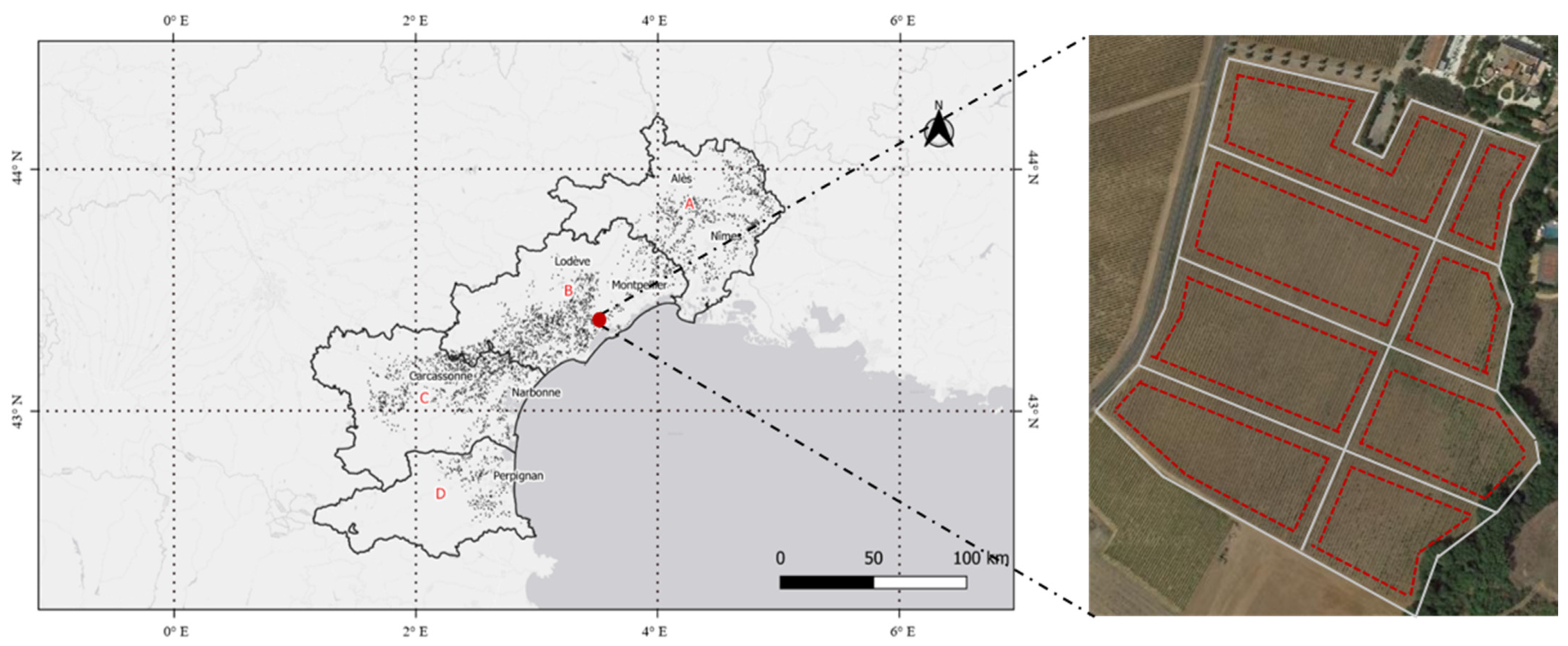
The study area corresponded to 4978 samples (vineyard blocks) extracted from the graphical parcel register of France (RPG) from a large wine-growing region located in southern France, the Languedoc-Roussillon (LR). The LR vineyards extend over approximately 27,400 km², covering four French administrative sectors: Gard (A), Hérault (B), Aude (C), and Pyrénées-Orientales (D) (Figure 2). The study area encompasses a great variability of pedo-climatic conditions and a great diversity of varieties, training systems, etc. [20]. It is assumed that changes in the reflectance values from Sentinel-2 satellites over the 4978 vineyard block samples over time will provide agronomic insights that arise from differences in the genotype–environment–management interactions between vineyards, locally and regionally. Assuming that a unique solution can be expected if the Sentinel-2 data are trilinear, i.e., that there is a relationship between the three-way structure of these data (samples × times × wavelengths) this would imply that the true pure spectra can be found if the correct number of components is used and the signal-to-noise ratio is appropriate [11].

2.3.2. Remote Sensing Data

The Sentinel-2 (A/B) satellites provide 13 spectral bands from the Visible (Vis) and Near InfraRed (NIR) to the shortwave infrared (SWIR) regions of the electromagnetic spectrum. They provide coverage of land surfaces on a global scale with a revisit frequency of 5 days in cloud-free conditions with a spatial resolution of 10, 20, or 60 m depending on the spectral band [21].

Sentinel-2 L2A data containing the study vineyards (Figure 2) were selected and processed via the Google Earth Engine (GEE) platform. Prior to the calculation of the average pixel values for each vineyard block, each date and each waveband, a 10 m inner buffer was imposed over each block boundary (Figure 2) that was extracted from the RPG. This 10 m inner buffer was used to prevent information from outside the block being integrated into the analysis [22]. Images from 1 May to 31 August in 2019 and 2020 were selected. This time period (from May to August) for both years of the study was considered as being the most relevant for monitoring vine vegetation in the study region [21]. Images containing clouds or shadows that altered the visibility of the blocks were removed from the database. For this purpose, the spectral band 10 at 1380 nm was used for the detection of visible and sub-visible cirrus clouds [23]. Approximately 25 images should have been available on each vineyard block over the two years; however, because of local atmospheric effects on the imagery, the final Sentinel-2 database consisted of 4978 vineyard blocks containing 12 spectral bands and an average of 11 images (dates) per block.

2.4. Modelling

2.4.1. Data Array Construction

Two PARAFAC models were derived from the data set of 4978 samples (vineyard blocks), one for each year of the study, 2019 and 2020. To overcome the challenge of heterogeneity in the number of images per block, an interpolation was performed to obtain two continuous data cubes; X₁₉ and X₂₀. Interpolation using the Gaussian filter by Alam et al. (2008) [24] was applied in order to have a consistent time step dimension (J) between 1 May and 31 August for both years. The parameters involved in the interpolation setting were fixed to the Gaussian filter width (P) = 30 days and date interval (N) = 5 days to simulate the revisit time of the Sentinel-2 satellites [22]. At the end of the interpolation step, the data set was meaningfully arranged in two three-way arrays X (X₁₉ and X₂₀) of dimensionality 4978 (samples, I) × 25 (times, J) × 12 (wavelengths, K).

2.4.2. PARAFAC Model

A separate decomposition of the two arrays, X₁₉ and X₂₀, into trilinear components was performed using the PARAFAC method. The trilinear model was found to minimize the sum of squares of the residuals, E_ijk in the model. Each component consisted of one score vector and two loading vectors, i.e., temporal and spectral loadings. A PARAFAC model of a three-way array, e.g., X₁₉, was given by one score matrix A and two loading matrices, B and C, with its respective $a_{if}$, $b_{jf}$, and $c_{kf}$(Figure 3). The parameter $a_{if}$ is the score of the ith sample of the fth component; $b_{jf}$ is the loading specific to reflectance intensity at the time j of the fth component; and $c_{kf}$ is the loading estimate of the reflectance spectrum k of the fth component. Essentially, the PARAFAC model provides an estimation of the relative concentration, i.e., the relative amount of the fth component in each sample (matrix A) and temporal and spectral properties of the components loadings matrices (B and C respectively), which can be used to interpret the spectral dynamics of the constituents of the samples. For 2020 (X₂₀), the same PARAFAC decomposition scheme was used as for 2019.

2.4.3. Component Selection

Several PARAFAC models, with the number of components in the models ranging from one to five, were fitted to the data in order to determine the model with the optimal number of components. A F-component model was validated following the Core Consistency Diagnostic (CORCONDIA) of Bro (1997) [11]. The PARAFAC model is considered to be valid if the value of the CORCONDIA is close to 100%. If the CORCONDIA value is around 50%, the model is considered unstable, and if the value is close to 0 (even negative), then it is considered that the data cannot be described by the tri-linear model [14]. The CORCONDIA value will mostly decrease with the number of components. It decreases very sharply after the optimal number of components is exceeded. Therefore, the appropriate number of components is the model with the highest number of components and a valid CORCONDIA value.

2.5. Validation of the Model

The PARAFAC models for both 2019 and 2020 were validated in two steps:

• A geostatistical analysis (see next section) to test whether the score values were spatially autocorrelated. The underlying hypothesis is that the environmental variables (soil, climate, and associated training practices, etc.) that are likely to explain the differences between blocks at the regional scale are spatially organised (not random). Consequently, if score values resulting from the PARAFAC models are not randomly distributed at the regional level, they are assumed to be related to environmental variables.
• An assessment of the coherence of the spatial distribution of the score values against expert knowledge of the diversity and spatial distribution of soil, climate, and vineyard cultural practices in the region. The objective of this second step was to identify the relevance of the relationship between the scores and agri-environmental information. In order to do so, an original approach based on placing the human, i.e., local viticultural experts, at the centre of the study was conducted. Following the methodological framework of Pichon et al. (2019) [12], a global approach, a so-called ‘scenario simulation’ [25], was used. In this method, external reliability can be considered valid if the conclusions reached by different experts (at least two experts) coincide [26,27]. In order to facilitate the expert’s interpretation, maps of score values were produced at the regional level. These maps were created by interpolating (see next section) the scores observed on the 4978 vineyard blocks for each year (2019 and 2020) and for each component (F) when spatial autocorrelation was observed.

2.6. Spatial Analysis and Mapping

The spatial analysis was based on the modelling of semivariograms, which allows for a statistical assessment of how spatially autocorrelated the data (scores) are over space. It is expected that the (semi)variance of points closer together will be lower if the data exhibits spatial patterning. From the semivariogram modelling, the following parameters were derived: C₀ (nugget effect or semivariance at a distance approaching 0 m), C₁ (sill or the maximum semivariance observed), and A₁ (the range (distance) at which C₁ is reached). The C₀ and C₁ parameters were first used to calculate the Cambardella Index [28] to determine the spatial dependence and then all three parameters were used in a kriging process to obtain the score maps. The characterisation of the spatial structure via semivariograms, as well as the realisation of the score maps, was performed using the GeoFis 1.0 software (Open Source Software GeoFIS, http://www.geofis.org, accessed on 24 August 2022) [29].

Spatial auto-correlation of the score values of each component was assessed with the Cambardella Index (I_c) [28] (Equation (2)):

$${\mathrm{I}}_{\mathrm{c}}=\frac{{\mathrm{C}}_0}{{\mathrm{C}}_0+{ \mathrm{C}}_1}$$

(2)

where C₀ is the nugget effect and C₁ is the sill of the semivariogram model. According to Cambardella et al. (1994) [28], the following thresholds were used:

• if I_c is less than or equal to 25%, the distribution is considered strongly spatially organised (high auto correlation);
• if I_c is between 25 and 75%, the distribution is considered moderately spatially organised; and,
• if I_c is higher than 75%, the distribution is considered weakly spatially organised.

Score maps were obtained using point kriging interpolation [30]. The latter was performed on a grid of points regularly spaced 1000 m apart within the geographical boundary of the LR region [31].

2.7. Experts Evaluation

Following Pichon et al. (2019) [12], 6 experts were selected. These 6 experts were chosen in order to benefit from an integrated assessment of the results obtained over the whole region, taking into account simultaneously their knowledge of plant development, the cultural practices of the winegrowers in each part of the region, the soil and its variability, etc. (see Supplementary Materials section).

In order to validate the experts’ consistency, they conducted a self-assessment of the criteria considered important by the authors for the study (

Table 1. Description of the interviewed domain experts. Ratings range from 0 to 5, with 0 being the minimum and 5 the maximum knowledge/expertise. The term Vegetation Indices is abbreviated as VIs.

	Experience Grapevine Cultivation				Knowledge of Viticulture of the LR Region				Knowledge of Pedo-Climatic Characteristics of the LR Region		Expertise with Remote Sensing Images
Expert	Vine Physiology	Irrigation	Technical Itineraries	Climate Impact	Aude (A)	Gard (B)	Hérault (C)	Pyrénées-Orientales (D)	Soil Type	Micro-Climate	Data Processing	VIs	Resolution Scale
A1	5	5	4	4	4	2	4	3	2	2	3	4	3
A2	4	3	3	3	3	3	4	4	3	3	4	4	4
A3	4	4	4	4	1	3	2	1	3	3	1	2	1
A4	4	5	4	4	4	4	4	4	4	4	4	4	1
A5	2	1	3	2	3	1	5	1	5	5	1	1	3
A6	4	5	5	4	4	4	4	3	4	3	3	5	4

). In this self-assessment, the experts ranked their perceived expertise on aspects of vineyard production, regional viticulture practices, regional pedo-climatic knowledge, and RS expertise on a scale from 0 (none) to 5 (excellent). This information validated the choice of experts and was also used to consider the importance of (i.e., weight) the different opinions expressed by different experts during the working session. For example, less importance was assigned to the opinion of expert A3 when assessing the scores in the Aude department due to A3 self-identifying as having a poor knowledge of viticultural practices in this department.

A ‘scenario simulation’ session was conducted with experts on 31 May 2022. The general workflow of the session is presented in

Table 2. Description of the general workflow of the ‘scenario simulation’ session.

	Step 1	Step 2	Step 3	Step 4	Step 5
Duration	40 min	20 min	40 min	20 min	40 min
Type of session	Individual (written)	Individual (written)	Collective (oral)	Collective (oral)	Collective (oral)
Presentation of maps	Once at time for the year 2020	All together for the 2020 year	Once at time for the year 2020	All together for the 2020 year	All together for the years 2019 and 2020

. During the session, the score maps were hand-delivered to each expert and projected on a screen managed by an animator (zoom in and out) according to requests from the experts. These score maps were previously elaborated by adding characteristic elements (cities, watercourses, roads, etc.) that would allow the experts to orientate themselves on the maps. It should be noted that an explanation session of the meaning of the score values was necessary so that the experts could understand the maps and interpret them in the best possible way using a colour coding defined by the authors. Maps were displayed in QGIS 3.2.3 (Open Source Geospatial Foundation, http://qgis.osgeo.org, accessed on 24 August 2022). Experts were asked to first write down their opinions before oral group discussions. In the oral group discussion, the animator wrote down the experts’ comments and reactions.

It was agreed that the experts would react mainly to score maps derived from the 2020 data, because it was considered to be most representative of common crop–soil–climate interactions in the region. In contrast, 2019 was assumed to present a specific atypical behaviour (although interesting) as a heatwave strongly affected vine growth in the region at the end of June. Score maps from 2019 were then presented in a second step as a particular case study.

3. Results

3.1. Component Selection

Table 3. Results of the CORe CONsistency DIAgnostic (CORCONDIA) after fitting a series of models using two to five components for the X₁₉ and X₂₀ databases.

Year	Number of Components (F)	CORCONDIA (%)	Variance Explained (%)
2019	1	100	99.25
2019	2	100	99.62
2019	3	15.65	99.74
2019	4	−6.34	99.82
2029	5	−0.72	99.88
2020	1	100	99.20
2020	2	100	99.57
2020	3	11.15	99.68
2020	4	−0.23	99.79
2020	5	−0.44	99.85

presents the results of fitting the PARAFAC model with different numbers of components (1–5) to X₁₉ and X₂₀. With two components, the observed CORCONDIA and explained variance values were 100–99.62% and 100–99.57% for 2019 and 2020, respectively. For a higher number of components, the CORCONDIA values dropped significantly, showing that the two-component model was the best for both years, as the appropriate number of components corresponded to the model with the highest number of components and a valid CORCONDIA value. Since a two-component model was validated according to CORCONDIA, the results in Table 3 also justified the suitability of applying the PARAFAC methodology assuming a trilinear structure in the presented data set.

3.2. Data Signal Decomposition

A two-component PARAFAC corresponds to two pure spectra of constituents. For both PARAFAC models (2019 and 2020), the score in the matrix A (4978 × 2) contains estimated relative concentrations in relation with both loadings (temporal × spectral) of the two components in the 4978 samples. The matrix B (25 × 2) contains estimated temporal loadings and the matrix C (12 × 2) estimated spectral loadings.

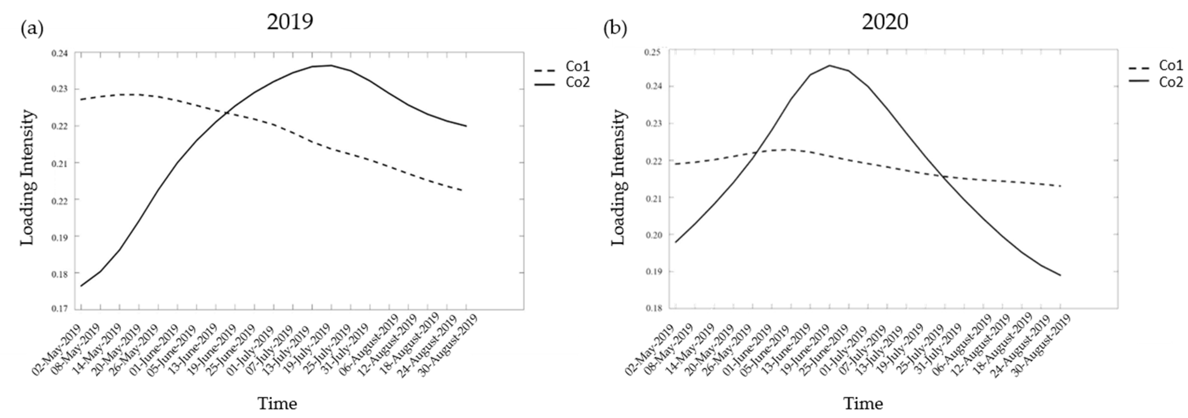
The spectral loadings (C) and the temporal loadings (B) for the two components selected (Co1 and Co2) from the PARAFAC model of the years 2019 and 2020 are presented in Figure 4 and Figure 5, respectively.

Regarding component 1 (Co1) for both years, it was observed that the loading intensity was characterised by an increase from the Visible (Vis) to the Near InfraRed region (NIR). It should be noted, though, that in 2019 there was a slight drop in intensity between the wavelengths ranging from 700 to 1000 nm. Concerning Co2 for both years, the spectral loading was characterised by: (i) a low intensity in red wavelengths (650–680 nm), (ii) the highest intensity in the NIR range (785–875 nm), and (iii) a decrease in intensity in the short-wave infrared region (1360–2200 nm). Taking into account that matrix C represents the pure spectra and considering the type of case study proposed, the components were identified as soil (Co1) and vegetation (Co2). Soil spectral reflectance is typically characterised by a steady increase with wavelengths from the Vis to the NIR, except at 950, 1200, and 1350 nm, where reflectance decreases [32]. As for the typical vegetation spectral reflectance, it exhibits the following characteristics: (i) a low reflection in the blue (458–523 nm) and red wavelengths (650–680 nm), (ii) relatively more reflection in green wavelengths (543–578 nm), (iii) reflectance in the NIR range (785–875 nm) is the highest, and iv) the short-wave infrared region (1360–2200 nm) is mainly characterised by less reflectance [33]. Given that grapevine cultivation is seasonal and is a row crop, the PARAFAC model clearly identifies the mixture of these two components. In fact, for both years, the Co2 spectral loadings represented a ‘reference’ vegetation profile (which refers to the notion of the pure spectra in chemometrics) that probably included both vines and interrow grass/crops reflecting the typical signature of healthy vegetation, while the Co1 spectral loadings represented a ‘reference’ soil profile at the region level. It actually summarised different soil types across the region, probably with different spectral characteristics. This may explain why the spectral loading identified as soil followed a slightly different general trend than that described as a typical soil profile by Khadse (2012) [32].

Figure 5 presents the temporal loadings (B) for both 2019 and 2020 and both components (Co1 and Co2). It was observed that the two components showed large differences between them in their temporal loadings in the two consecutive years. Regarding Co1, in 2019 the intensity in its time profile decreased over time, while in 2020 it remained more stable. Regarding Co2, its spectral profile in 2019 peaked between 17 and 27 of July, with a slow decrease afterward, while for 2020 the Co2 showed a maximum around 11 and 26 of June followed by a very steep decline later in the season. Indeed, the temporal loadings of both years seemed to show that the Co2 intensity (vegetation) increased with the vegetative development of the vine (June-July) and, conversely, Co1 intensity (soil) decreased with the growth of the vine. In fact, the decreasing temporal profile of Co1 observed throughout 2019 reaffirms the hypothesis that it may be a compensatory profile of the vegetation at certain times during the time period considered. For the record, 2019 was marked by a heatwave in late June that affected a significant part of the region, which may explain a compensatory effect later in the season. With regard to Co2, the maximum peak of intensity shifted between 2019 and 2020, moving forward by almost one month in 2020. This could be explained if the time of vegetative development (phenological stages) of the vineyards was different between the two years studied.

Given that the samples studied were vineyard blocks, the spectral and temporal profiles indicate a ‘reference’ behaviour for each component (soil and vegetation) at the regional scale, but each block may differ more or less from this ‘reference’ behaviour. Thus, once the models were validated, the data could be examined with respect to the variability of each component found, i.e., with respect to the values of the score matrix (A) for both years.

3.3. Spatial Analysis and Characterisation

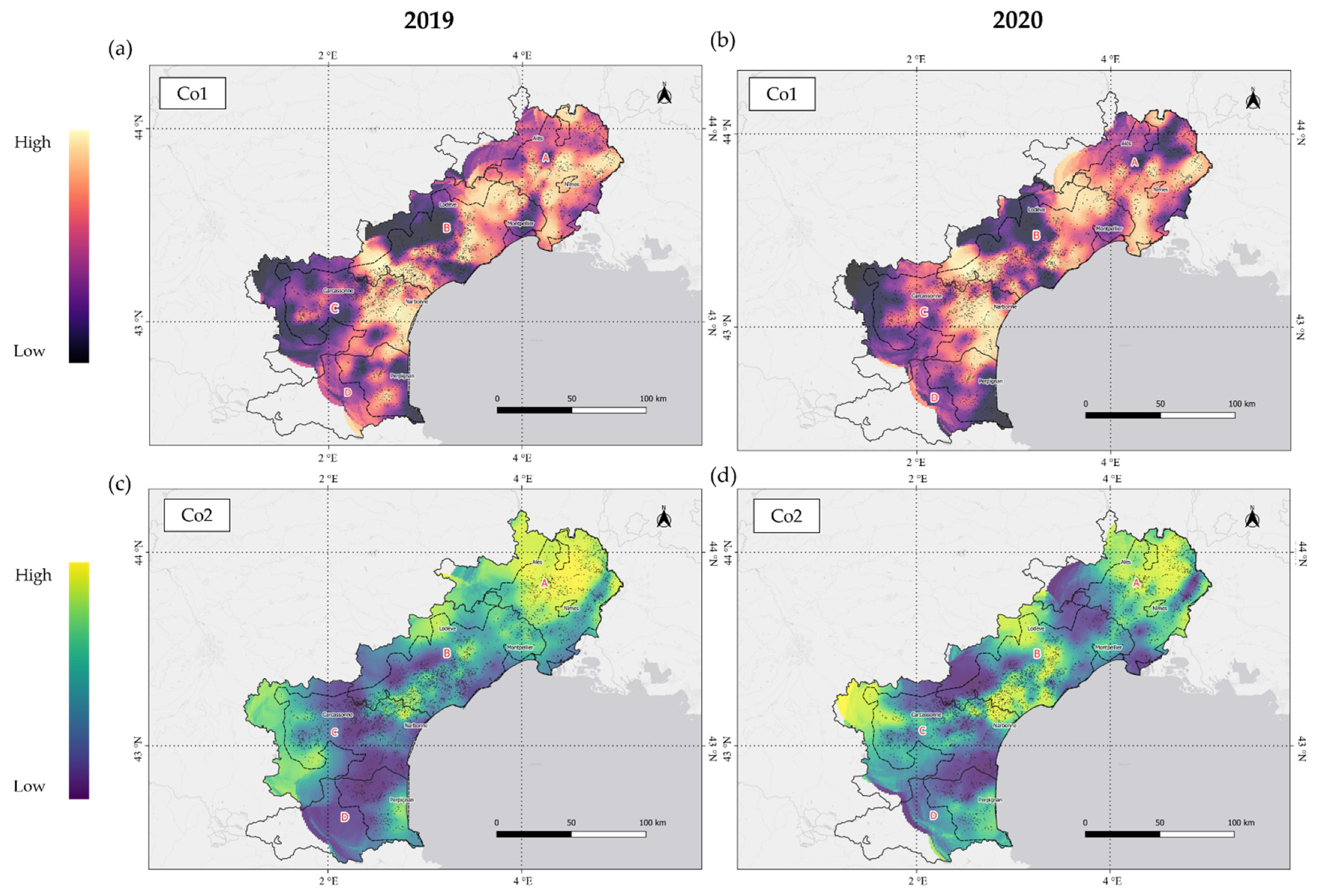
The score value maps (Figure 6) represent the spectro-temporal scores of each block in relation to each component and its corresponding year, e.g., for Figure 6a, the estimated concentration value of the Co1 (soil) component of each block is plotted in relation to its spectro-temporal profile in 2019 at the regional level. Therefore, the score map for Co1 was supposed to highlight blocks that were directly related (or counter-related) to the identified spectro-temporal signature for the soil in 2019.

The spatial organisation of the score maps for both years and for all the selected components was confirmed by the semivariogram modelling (

Table 4. Semivariogram parameters and spatial variability index for score values. A₁ (Range), C₀ (Nugget), C₁ (Sill), and I_c (Cambardella Index).

Year	Components	Semivariogram Model	A1 (Km)	C0	C1	Ic (%)
2019	Co1	Exponential	6	0.067	0.079	45
	Co2	Exponential	6	0.026	0.022	53
2020	Co1	Exponential	5	0.205	0.113	64
	Co2	Exponential	5	0.145	0.086	62

), which showed that at least 40–50% of the variability was explained by a spatial phenomenon. The year and component with the strongest spatial structure was the soil component (Co1) for 2019 with an I_c of 45%. These results support the assumption that scores values were not randomly organised, but spatially structured and likely to vary according to environmental variables.

The score maps obtained after kriging (Figure 6) show the spatial organisation of the blocks that have: (i) a similar spectro-temporal profile (high scores) and (ii) a different spectro-temporal profile (low scores) to the ‘reference’ spectral profile for each component and year. Therefore, the greater the difference in the time spectral profiles, the lower the scores, which were negative if they were opposite to the ‘reference’ spectro-temporal profile. The spatial patterns for soil (Co1) between the two years were very similar, showing that the same vineyard blocks had both high (light colour) and low (dark colour) score values in the same areas for both years. Regarding the spatial patterns of vegetation (Co2) for both years, a general trend of higher score values (light colour) in the northern part of the region was highlighted. For other sectors, the spatial patterns were less similar between both years. It should be noted that, for Co2, the spectral loadings (Figure 4) followed the same profile in both years but, in contrast, the temporal loadings (Figure 5) showed a significant temporal shift. This implies that the temporal dimension may have a major role in the difference in score values for each vineyard block for both years, i.e., in the differences in spatial patterns for each year represented.

3.4. Comparaison of Cross-Observation by Experts

Regarding the spatial patterns for Co1 between 2019 and 2020, these were almost identical (Figure 6a,b), and it was considered that the score map of Co1 for 2019 would not provide any relevant information to the study for the experts. Therefore, the workflow of cross-validation by experts focused first on the two 2020 components (Co1 and Co2), and then the vegetation component (Co2) from 2019 was presented only for comparison with 2020.

Table 5. Number of experts who made similar observation in each sector of the LR region for the Co1 and Co2 score maps for the year 2020.

Component	Figure Number	Observations on	Sector A	Sector B	Sector C	Sector D
Co1 (Soil)	Figure 7a	Variation of pedological units	5	5	2	1
	Figure 7b	Variation of geological units	5	4	4	0
Co2 (Vegetation)	Figure 8a	Differences in grape varieties (phenology)	4	2	3	1
	Figure 8b	Variation of vine vigour	2	1	3	1
	Figure 8c	Presence/absence of irrigation	4	4	1	1

presents the extent to which each type of observation was made by the expert group for the 2020 year.

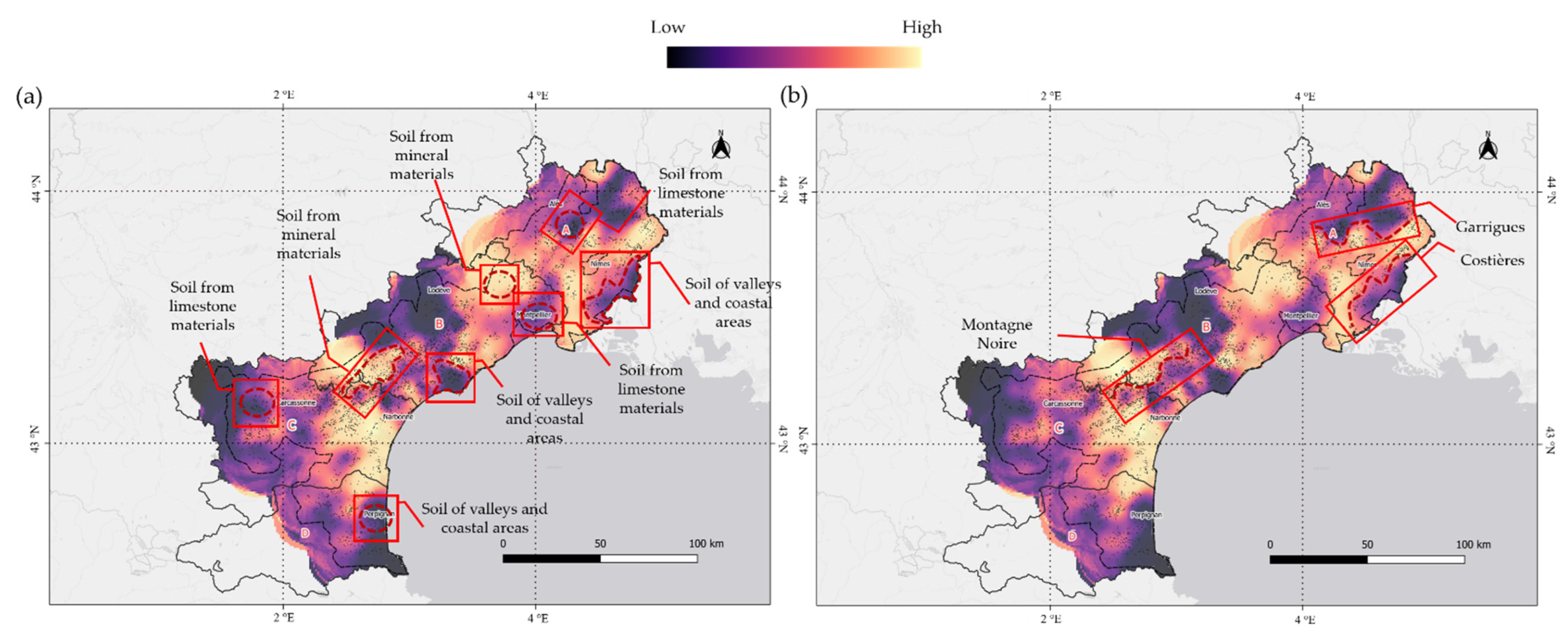
It clearly appears that a significant number of experts made similar observations on Sectors A and B of the LR region. Moreover, more expert observations were related to Co1 than to Co2. This result can be explained by the scale of the study, where vegetation heterogeneity may be more difficult to analyse properly by the experts given the large diversity of situations. Experts were obviously more comfortable with identifying and explaining differences in spatial patterns within sectors that they were familiar with. Figure 7 shows a summary map of each type of observation for 2020 made by the group of experts related to Co1 for each sector.

The observations made by individual experts coincided in the vast majority of cases with at least one other expert. Therefore, if at least two experts were in agreement, the relevance of the identified area was considered valid, according to Wacheux (1996) [25]. Concerning the soil units (Figure 7a), experts identified that the spatial patterns were related to the depth of the soil. In terms of colour range, it was perceived that the darker areas could represent valley and coastal soils, e.g., fluviosols, as well as calcareous soils. The former are soils containing mostly coarse elements (gravel, pebbles, stones, etc.) with a thickness >0.50 m and the latter are defined as medium to thick soils (>0.35 m thick), developed from calcareous materials. By comparison, the lighter zones (less distinct from a visual point of view) could represent mineral soils, e.g., rankosols or lithosols, which are characterised by a thickness of <0.30 m. It should be noted that this spatialisation of the different geological units was directly related to the information on the soil available water capacity provided by four experts. Regarding Figure 7b, some major geological formations within the LR region were largely commented on by five of the experts. Three clear boundaries between the two colours were observed and are outlined in sectors A-B-C of the map.

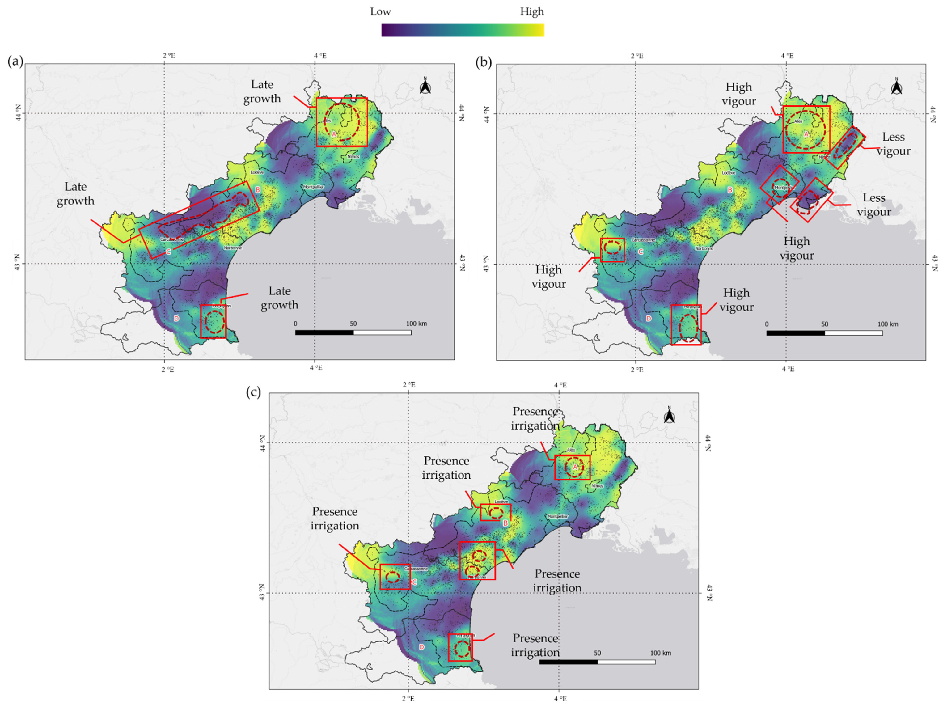
Regarding Figure 8 (Co2), it should be noted that the colour coding does not always represent the same phenomenon, but rather differences when compared to the ‘reference’ spectro-temporal profile for 2020. That is, the yellow vineyard blocks represent a spectro-temporal profile very similar to the ‘reference’ vegetation profile extracted by the PARAFAC method. In contrast, the blue vineyard blocks represent plots that differ from the ‘reference’ spectro-temporal profile of the vegetation. Therefore, as these colour variations may be due to differences in the spectral and/or temporal profiles in relation to the ‘reference’ profile, there were some inconsistencies in the experts’ interpretation of the meaning of the colour codes. A clear example was the comments on the phenological state of the vineyards by sectors in Figure 8a. Each of the areas highlighted in Figure 8a was selected by the experts as characteristic of late growth vineyard development, but the colours were different in each area. These inconsistencies could be explained, not by the late phenological stage, but by the different grape varieties selected and adapted to this late growth in each sector, e.g., a predominance of Chardonnay in sector A and a predominance of Mourvèdre in sector C. Since the grape varieties were different, different management practices, different training systems, etc., could be involved, and thus explain why on some maps the observed trends and the resulting agronomic interpretations were difficult to interpret.

Concerning Figure 8b, certain spatial structures, which were characterised by high/low vine vigour, were commented on by a minority of the experts. A possible explanation given by one of the experts focusing on sector A was the presence of the distinct denomination areas that characterise the different vineyards. In particular, the yellow area corresponded to the Protected Geographical Indication (PGI) label and the blue area to the Protected Designation of Origin (PDO) label. Two different identifications imply different yield objectives, soil cultivations, grape varieties, and management practices. The latest observations made by the experts are shown in Figure 8c and concern zones where irrigation is available through regional facilities. The experts largely addressed these observations for sectors A and B.

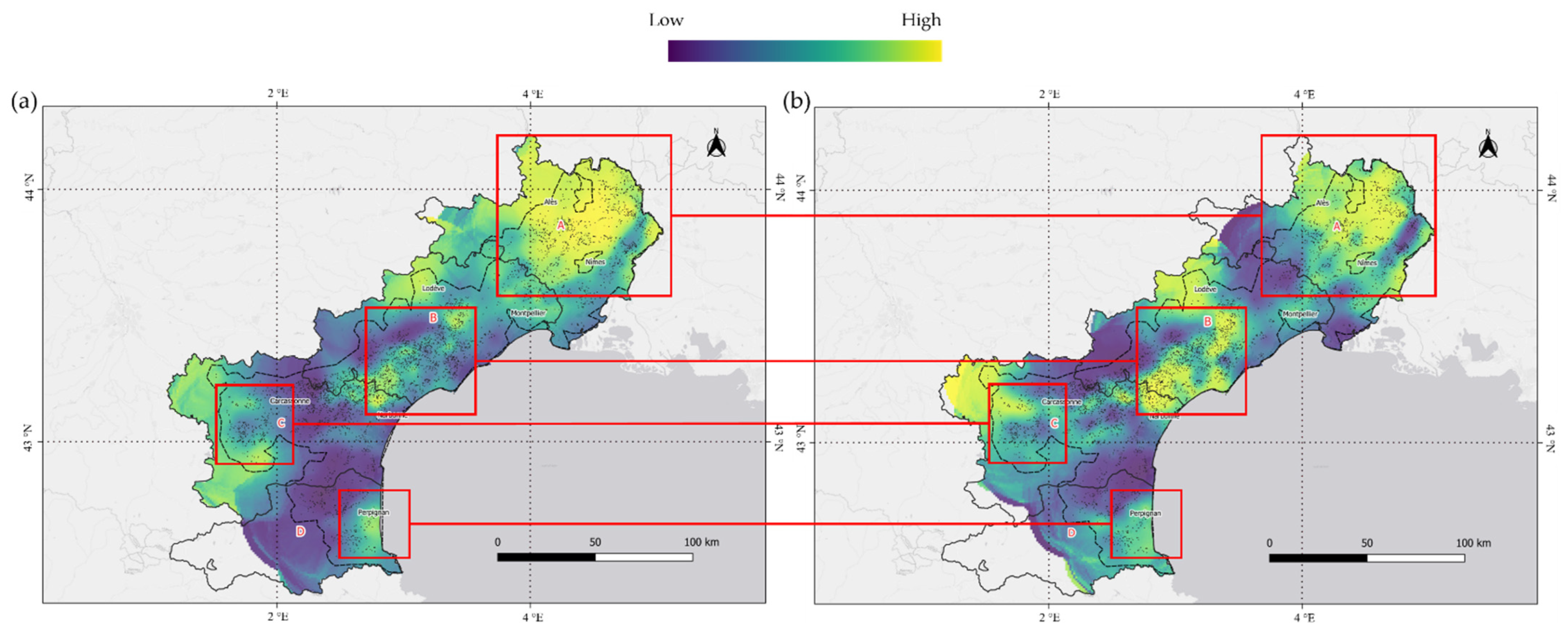
For the final step of the workflow (Table 2) it was decided to present only the score map from 2019 for the vegetation component (Co2) as the score map of the Co1 confirmed the stability of this component from one year to another, and the temporal stable factors (mainly related to soil) that it is related to. Therefore, when comparing the two years for the Co2 component, the experts observed the same spatial patterns but noted that these were less pronounced in 2019 (Figure 9a). This attenuation of the yellow colour, associated with higher score values, could be justified by the heatwave episode from 23 June to 8 July in 2019 that was experienced in the LR wine-growing region. The heatwave would have homogenised the differences between vineyards and, therefore, the corresponding spectro-temporal profiles.

4. Discussion

A remote sensing time series study for the regional characterisation of vineyard blocks was provided by the application of the PARAFAC algorithm. Results showed both the potential and the limitations provided by the application of an unsupervised complex data analysis method focusing on grapevine production at the regional scale. The validated application with a practical framework of expert winegrowers’ opinions demonstrated both the complexity and the added value of considering the feature approach in the temporal and spectral dimensions for interpretation purposes to identify relevant region/local characteristics in a grapevine context.

In order to analyse a time series of multispectral images to assess the value of simultaneously considering spectral and temporal information over the LR wine-growing region, the PARAFAC method was used to address the issue of analysing the three-way Sentinel-2 data sets in two distinct years, 2019 and 2020. It should be noted that a trilinear structure was assumed a priori in the analysis of the data sets. This assumption could be partly accepted because the fit of the data obtained was satisfactory according to the CORCONDIA criterion (100% for both years) and because the shape of the spectro-temporal profiles obtained was coherent from an agronomic point of view. Several authors, including De Juan and Tauler (2001) [34], have established that methods based on the trilinear structure assumption will fit the data less efficiently than others that do not, such as Tucker3 [35] or Multivariate Curve-Resolution Alternating Least Squares (MCR-ALS) [36]. Indeed, the more ambiguous solutions given by Tucker3 and MCR-ALS through bilinear decomposition are balanced by the greater flexibility in modelling the shape of the profiles, which also leads to a feasible physical and chemical interpretation of the results [37]. However, the applicability of these kind of methodologies, which assume linear relationships in the data, is basically unknown in remote sensing scenarios. This is because the definition of the component, i.e., soil, vegetation, etc., and the image acquisition conditions will sometimes justify the assumption of a certain variability in the spectral signatures of the components [38]. Therefore, the non-linear unmixing, which is essentially the usual approach used in remote sensing, is often solved using deep learning methods [38]. Regardless of this claim, the PARAFAC decomposition accurately modelled soil dynamics and vegetation dynamics for both 2019 and 2020. The interpretability of the spectro-temporal profiles was useful to understand the variation of the spectral response of crops (soil-vegetation dynamics) over time.

Since the PARAFAC decomposition allowed for unique solutions to be obtained, i.e., pure spectra, the modelling was considered relevant for the study of the temporal dynamics of vineyard blocks at the scale of the region. However, it is essential to place the results presented in this paper within the reality of large-scale unsupervised case study data. It was apparent that the study of such variable samples that are representative of a large geographical area has limitations related to the reliability of the validation. To overcome this challenge, Wacheux’s (1996) [25] ‘scenario simulation’ was used, where if at least two experts confirmed that there is some logic in the observations, then these observations are considered valid. The proportion of different experts who made the same observation for each score map for the year 2020 can be considered a reliable indicator of the representativeness of the findings and may validate the relevance of the approach in highlighting relevant agronomic information. The observations were not made in the same proportion or in the same detail for the different sectors of the LR region. Table 5 clearly shows that almost all the observations in sector D were made by only one expert. This does not question the approach, but given the observations of the selected experts, it is to be expected that the conclusions from sectors A, B, and C were more consistent than those from sector D, where only one expert had in-depth knowledge. However, it should be highlighted that the ‘external reliability’ of this study refers to the LR region and that the same validation framework would have been approached differently, i.e., with experts from other regions or different countries, if a different scale of study had been defined.

Chemometric data analysis methods use very little a priori knowledge. Instead, they provide parameters that give insight into the system, such as its intrinsic dimension or the loadings that describe it. However, their relevance must be verified by numerical criteria and the user’s expertise. Thus, for the PARAFAC method, the number of factors is a result of the decomposition. It must be chosen by successive trials of increasing size, examining criteria, such as CORCONDIA, and also examining the relevance of the loadings produced. For other factorial methods, such as PCA [39], PLS [40], or MCR-ALS [36], the explained variance, prediction error, or lack of fit will be examined respectively. In analytical chemistry, the systems are often simple. In these cases, some priors can be useful for the calculation of the model. In agriculture, situations are often very complex, and it is difficult to constrain the model. Therefore, the result of the model must be verified a posteriori.

The main limitation of the PARAFAC methodology in relation to its application with Sentinel-2 satellite data at a regional scale is that it required a temporal interpolation step prior to the analysis in order to create a continuous data cube. However, this step necessarily involved a smoothing of the spectral data, which could lead to the removal of relevant information for crop monitoring. In addition to the methodological limitation mentioned above, there was also an important limitation within the expert’s validation framework used. Indeed, the spatial representation of a single score value summarising the whole growing season (the same colour code represents in reality a large variety of phenomena), probably added complexity to the interpretation by experts of areas related to ‘real’ soil or vegetation dynamics. However, according to the experts, the PARAFAC analysis highlighted different, relevant zones according to their knowledge. From the differences in the score value maps, different spatial patterns were visually highlighted that could potentially reveal some interpretative clues depending on the situation of the vineyards (geographical area, soil characteristics, and soil water capacity), the different phenological stages of the vineyards (different denominations area, grape variety, and management practices), and the impact of the use of irrigation in certain areas.

The validation of the results was only performed at the regional scale with a group of experts able to integrate a wide range of knowledge (soils, crops, climates) to analyse the relevance of the information obtained. It is likely that similar analyses conducted at finer scales will identify new information and perhaps even interesting links to new agronomic information. However, the availability of such experts, at both regional and local scales, to perform this validation is a potential limitation of the approach. In their absence it will be difficult to correctly extract and identify the various agronomic and pedo-climatic effects from the model outputs.

Concerning the year 2019, the validation by the expert group focused only on the vegetation component, highlighting its similarity, i.e., same spatial patterns with the subsequent year. The main observation was the attenuation of the high-value zones in 2019, which raised the hypothesis that the crop-heatwave interaction caused the homogenisation of the reflectance signal, creating a less differentiated spatial distribution of vine vigour at the regional scale in 2019, i.e., fewer strong concentration values (yellow colour). However, no sudden variations in the profiles were observed, as would be expected as a consequence of the impact of an extreme weather event. This could also be attributed to the fact that the temporal interpolation performed may have masked this punctual variability.

The unsupervised approach (PARAFAC) presented here represents a specific application case for the LR wine-growing region in 2019 and 2020. In view of the results, it is a type of approach that can be effective for spatialising and characterising phenomena with a temporal evolution, e.g., the spectral response of the vine canopy, providing spectro-temporal ‘fingerprints’ that are capable of highlighting differences in behaviour. However, in this particular case study, probably as a consequence of the resolution scale, its application is dependent on a posteriori expert knowledge of the observed phenomenon, thus limiting its applicability.

5. Conclusions

The work conducted in this study showed the potential of an appropriate three-way data resolution methodology, such as PARAFAC, in the analysis of remote sensing images time series. The results obtained from data collected over two cropping years (2019–2020), on 4978 vineyard blocks showed that the PARAFAC method provided relevant information on temporal spectral profiles, which, in turn, allowed the spatial characterisation of the LR wine region. The validation of the results was based on expert observations. Although this can be seen as a limitation, the practical approach of experts demonstrated that the application of specific methodologies for the resolution of complex three-way data can be optimised at various levels and be potentially useful for understanding and characterising viticulture at the regional scale. Elements extracted from the PARAFAC method, such as the relationship with the landscape, the irrigation areas in relation to the soil characteristics, and the spatial footprint of the soil water capacity seen as an indicator of biomass production over the season, have given the authors new insights into elements to be investigated in more detail. However, the requirement to have a continuous cube can be a limiting factor in characterising isolated episodes that affect the crop growth during the year.

The proposed methodology is potentially transferable to other resolution scales. In fact, for the effective characterisation of the specificity of the spectral temporal response of agricultural-related factors at other scales, the spatial segmentation elements (different spectral time zones) highlighted by the PARAFAC methodology and identified by expert observations would be appropriate as a starting point. It is assumed that the methodology is equally transferable to other regions and other cropping systems, although the resulting inferences will be very different.

References

1. Griffiths, G.H.; Lee, J. Landscape Pattern and Species Richness; Regional Scale Analysis from Remote Sensing. Int. J. Remote Sens. 2000, 21, 2685–2704. [Google Scholar] [CrossRef]
2. Gilbertson, J.K.; van Niekerk, A. Value of Dimensionality Reduction for Crop Differentiation with Multi-Temporal Imagery and Machine Learning. Comput. Electron. Agric. 2017, 142, 50–58. [Google Scholar] [CrossRef]
3. Weiss, M.; Jacob, F.; Duveiller, G. Remote Sensing for Agricultural Applications: A Meta-Review. Remote Sens. Environ. 2020, 236, 111402. [Google Scholar] [CrossRef]
4. Huang, Y.; Chen, Z.; Yu, T.; Huang, X.; Gu, X. Agricultural Remote Sensing Big Data: Management and Applications. J. Integr. Agric. 2018, 17, 1915–1931. [Google Scholar] [CrossRef]
5. Kroonenberg, P.M.; Harshman, R.A.; Murakami, T. Analysing Three-Way Profile Data Using the Parafac and Tucker3 Models Illustrated with Views on Parenting. Appl. Multivar. Res. 2009, 13, 5. [Google Scholar] [CrossRef] [Green Version]
6. Kiers, H.; Mechelen, I. Three-Way Component Analysis: Principles and Illustrative Application. Psychol. Methods 2001, 6, 84–110. [Google Scholar] [CrossRef]
7. Khanal, S.; Kc, K.; Fulton, J.P.; Shearer, S.; Ozkan, E. Remote Sensing in Agriculture—Accomplishments, Limitations, and Opportunities. Remote Sens. 2020, 12, 3783. [Google Scholar] [CrossRef]
8. Esbensen, K.; Geladi, P. Strategy of Multivariate Image Analysis (MIA). Chemom. Intell. Lab. Syst. 1989, 7, 67–86. [Google Scholar] [CrossRef]
9. Verbeeck, N.; Caprioli, R.M.; Van de Plas, R. Unsupervised Machine Learning for Exploratory Data Analysis in Imaging Mass Spectrometry. Mass Spectrom. Rev. 2020, 39, 245–291. [Google Scholar] [CrossRef] [Green Version]
10. Harshman, R. Foundations of the PARAFAC Procedure: Models and Conditions for an Explanatory Multi-modal Factor Analysis. UCLA Work. Pap. Phon. 1970, 16, 1–84. [Google Scholar]
11. Bro, R. PARAFAC. Tutorial and Applications. Chemom. Intell. Lab. Syst. 1997, 38, 149–171. [Google Scholar] [CrossRef]
12. Pichon, L.; Leroux, C.; Macombe, C.; Taylor, J.; Tisseyre, B. What Relevant Information Can Be Identified by Experts on Un-manned Aerial Vehicles’ Visible Images for Precision Viticulture? Precis. Agric. 2019, 20, 278–294. [Google Scholar] [CrossRef]
13. Yang, X.; Yu, X.; Cheng, J.; Zheng, R.; Wang, K.; Dai, Y.; Tong, N.; Chow, A. Impacts of Land-Use on Surface Waters at the Watershed Scale in Southeastern China: Insight from Fluorescence Excitation-Emission Matrix and PARAFAC. Sci. Total Environ. 2018, 627, 647–657. [Google Scholar] [CrossRef] [PubMed]
14. Ouertani, S.S. Nway Partial Least Squares: Nouvelles Propriétés et Apports à la Discrimination des Données Métabolomiques. Ph.D. Thesis, University of Geneva, Geneva, Switzerland, 2014. [Google Scholar]
15. Xu, X.; Kang, J.; Shen, J.; Zhao, S.; Wang, B.; Zhang, X.; Chen, Z. EEM–PARAFAC Characterization of Dissolved Organic Matter and Its Relationship with Disinfection by-Products Formation Potential in Drinking Water Sources of Northeastern China. Sci. Total Environ. 2021, 774, 145297. [Google Scholar] [CrossRef]
16. Andersson, C.; Bro, R. The N-Way Toolbox for Matlab. Chemom. Intell. Lab. Syst. 2000, 52, 1–4. [Google Scholar] [CrossRef]
17. Giovos, R.; Tassopoulos, D.; Kalivas, D.; Lougkos, N.; Priovolou, A. Remote Sensing Vegetation Indices in Viticulture: A Critical Review. Agriculture 2021, 11, 457. [Google Scholar] [CrossRef]
18. Zhou, Y.; Pei, F.; Xia, Y.; Wu, C.; Zhong, R.; Wang, K.; Wang, H.; Cao, Y. Assessing the Impacts of Extreme Climate Events on Vegetation Activity in the North South Transect of Eastern China (NSTEC). Water 2019, 11, 2291. [Google Scholar] [CrossRef] [Green Version]
19. Sozzi, M.; Kayad, A.; Marinello, F.; Taylor, J.; Tisseyre, B. Comparing Vineyard Imagery Acquired from Sentinel-2 and Un-manned Aerial Vehicle (UAV) Platform. Oeno One 2020, 54, 189–197. [Google Scholar] [CrossRef] [Green Version]
20. Fernández-Mena, H.; Frey, H.; Celette, F.; Garcia, L.; Barkaoui, K.; Hossard, L.; Naulleau, A.; Métral, R.; Gary, C.; Metay, A. Spatial and Temporal Diversity of Service Plant Management Strategies across Vineyards in the South of France. Analysis through the Coverage Index. Eur. J. Agron. 2021, 123, 126191. [Google Scholar] [CrossRef]
21. Devaux, N.; Crestey, T.; Leroux, C.; Tisseyre, B. Potential of Sentinel-2 Satellite Images to Monitor Vine Fields Grown at a Territorial Scale. Oeno One 2019, 53, 52–59. [Google Scholar] [CrossRef]
22. Lopez-Fornieles, E.; Brunel, G.; Rancon, F.; Gaci, B.; Metz, M.; Devaux, N.; Taylor, J.; Tisseyre, B.; Roger, J.-M. Potential of Multiway PLS (N-PLS) Regression Method to Analyse Time-Series of Multispectral Images: A Case Study in Agriculture. Remote Sens. 2022, 14, 216. [Google Scholar] [CrossRef]
23. Hollstein, A.; Segl, K.; Guanter, L.; Brell, M.; Enesco, M. Ready-to-Use Methods for the Detection of Clouds, Cirrus, Snow, Shadow, Water and Clear Sky Pixels in Sentinel-2 MSI Images. Remote Sens. 2016, 8, 666. [Google Scholar] [CrossRef] [Green Version]
24. Alam, M.S.; Islam, M.N.; Bal, A.; Karim, M.A. Hyperspectral Target Detection Using Gaussian Filter and Post-Processing. Opt. Lasers Eng. 2008, 46, 817–822. [Google Scholar] [CrossRef]
25. Wacheux, F. Méthodes Qualitatives de Recherches En Gestion; Economica: Paris, France, 1996; p. 290. [Google Scholar]
26. Shadish, W.R.; Cook, T.D.; Campbell, D.T. Experimental and Quasi-Experimental Designs for Generalized Causal Inference; Houghton Mifflin Company: Boston, MA, USA, 2002. [Google Scholar]
27. Drost, E. Validity and Reliability in Social Science Research. Educ. Res. Perspect. 2011, 38, 105–124. [Google Scholar]
28. Cambardella, C.A.; Moorman, T.B.; Novak, J.M.; Parkin, T.B.; Karlen, D.L.; Turco, R.F.; Konopka, A.E. Field-Scale Variability of Soil Properties in Central Iowa Soils. Soil Sci. Soc. Am. J. 1994, 58, 1501–1511. [Google Scholar] [CrossRef]
29. Leroux, C.; Jones, H.; Pichon, L.; Guillaume, S.; Lamour, J.; Taylor, J.; Naud, O.; Crestey, T.; Lablee, J.-L.; Tisseyre, B. GeoFIS: An Open Source, Decision-Support Tool for Precision Agriculture Data. Agriculture 2018, 8, 73. [Google Scholar] [CrossRef] [Green Version]
30. Oliver, M.A.; Webster, R. A Tutorial Guide to Geostatistics: Computing and Modelling Variograms and Kriging. Catena 2014, 113, 56–69. [Google Scholar] [CrossRef]
31. Lopez-Fornieles, E.; Brunel, G.; Devaux, N.; Roger, J.-M.; Tisseyre, B. Is It Possible to Assess Heatwave Impact on Grapevines at the Regional Level with Time Series of Satellite Images? Agronomy 2022, 12, 563. [Google Scholar] [CrossRef]
32. Khadse, G.K. Spectral Reflectance Characteristics of the Soils on Basaltic Terrain of Central Indian Plateau. J. Indian Soc. Remote Sens. 2012, 40, 717–724. [Google Scholar] [CrossRef]
33. Roman, A.; Ursu, T. Multispectral Satellite Imagery and Airborne Laser Scanning Techniques for the Detection of Archaeo-logical Vegetation Marks. In Landscape Archaeology on the Northern Frontier of the Roman Empire at Porolissum: An Interdisciplinary Research Project; Coriolan, H.O., Vlad-Andrei, L., Eds.; Mega Publishing House: Cluj-Napoca, Romania, 2016; pp. 141–152. [Google Scholar]
34. de Juan, A.; Tauler, R. Comparison of Three-Way Resolution Methods for Non-Trilinear Chemical Data Sets. J. Chemom. 2001, 15, 749–771. [Google Scholar] [CrossRef]
35. Tucker, L.R. Some mathematical notes on three-mode factor analysis. Psychometrika 1966, 31, 279–311. [Google Scholar] [CrossRef] [PubMed]
36. Tauler, R.; Smilde, A.; Kowalski, B. Selectivity, local rank, three-way data analysis and ambiguity in multivariate curve resolution. J. Chemom. 1995, 9, 31–58. [Google Scholar] [CrossRef]
37. Pomareda, V.; Guamán, A.V.; Mohammadnejad, M.; Calvo, D.; Pardo, A.; Marco, S. Multivariate curve resolution of nonlinear ion mobility spectra followed by multivariate nonlinear calibration for quantitative prediction. Chemom. Intell. Lab. Syst. 2012, 118, 219–229. [Google Scholar] [CrossRef]
38. Gómez-Sánchez, A.; Marro, M.; Marsal, M.; Zacchetti, S.; Rocha de Oliveira, R.; Loza-Alvarez, P.; de Juan, A. Linear un-mixing protocol for hyperspectral image fusion analysis applied to a case study of vegetal tissues. Sci. Rep. 2021, 11, 18665. [Google Scholar] [CrossRef] [PubMed]
39. Pearson, K. On Lines and Planes of Closest Fit to Systems of Points in Space (PDF). Lond. Edinb. Dublin Philos. Mag. J. Sci. 1901, 2, 559–572. [Google Scholar] [CrossRef]
40. Wold, S.; Martens, H.; Wold, H. The multivariate calibration problem in chemistry solved by the PLS method. In Matrix Pencils; Ruhe, A., Kågstrøm, B., Eds.; Springer: Berlin/Heidelberg, Germany, 1982; pp. 286–293. [Google Scholar]
Figure 1. Schema of the PARAFAC decomposition of a three-way array [14].
Agronomy 12 02544 g001
Figure 2. Location of the 4978 vineyard blocks within the study area in Southern France for the four administrative sectors: Gard (A), Hérault (B), Aude (C), and Pyrénées-Orientales (D). An example of vineyard blocks is provided with the addition of a red line on the inside indicating the 10 m inner buffer used to remove border effects (see Section 2.3.1).
Agronomy 12 02544 g002
Figure 3. Schema of the PARAFAC decomposition model of three-way array for the year 2019 (X19) where K represents relevant wavelengths, J represents time, and I represents the objects of interest, vineyard blocks in this case. E corresponds to the residuals.
Agronomy 12 02544 g003
Figure 4. Two-component PARAFAC models for 2019 and 2020 including spectral loadings (matrix C) for both components (Co1 and Co2). (a) 2019, (b) 2020.
Agronomy 12 02544 g004
Figure 5. Two-component PARAFAC models for 2019 and 2020 including temporal loadings (matrix B) for both components (Co1 and Co2). (a) 2019, (b) 2020.
Agronomy 12 02544 g005
Figure 6. Interpolated maps of the score values of each vineyard blocks at the regional scale for (a) component 1 (Co1) identified as the soil spectro-temporal profile in 2019 and (b) 2020; and component 2 (Co2) identified as the vegetation spectro-temporal profile in (c) 2019 and (d) 2020. Light colours represent high score values and dark colours represent low score values for both components. Interpolation was performed using ordinary kriging using the semivariogram information in Table 4.
Agronomy 12 02544 g006
Figure 7. The interpolated 2020 Co1 map overlayed with summary information (Table 5) that was identified by multiple experts and associated with effects attributed to: (a) the variation in the pedological units and (b) the variation in the geological units for 2020 made by the group of experts for each sector. Light colours represent high score values and dark colours represent low score values for Co1. Areas of the experts’ observations are highlighted in red squares.
Agronomy 12 02544 g007
Figure 8. The interpolated 2020 Co2 map overlayed with summary information (Table 5) that was identified by multiple experts and associated with effects attributed to: (a) the different grape variety (phenology effects), (b) variations in vine vigour, and (c) the presence/absence of irrigation. Light colours represent high score values and dark colours represent low score values for Co2. Areas of the experts’ observations are highlighted in red squares.
Agronomy 12 02544 g008
Figure 9. Visual comparison of the main spatial structures of the Co2 score maps for (a) 2019 and (b) 2020. Light colours represent high score values and dark colours represent low score values for Co2. Observations made by experts in 2020 that these same experts found in 2019 are highlighted in red squares.
Agronomy 12 02544 g009