An Object-Based Weighting Approach to Spatiotemporal Fusion of High Spatial Resolution Satellite Images for Small-Scale Cropland Monitoring

Abstract

Continuous crop monitoring often requires a time-series set of satellite images. Since satellite images have a trade-off in spatial and temporal resolution, spatiotemporal image fusion (STIF) has been applied to construct time-series images at a consistent scale. With the increased availability of high spatial resolution images, it is necessary to develop a new STIF model that can effectively reflect the properties of high spatial resolution satellite images for small-scale crop field monitoring. This paper proposes an advanced STIF model using a single image pair, called high spatial resolution image fusion using object-based weighting (HIFOW), for blending high spatial resolution satellite images. The four-step weighted-function approach of HIFOW includes (1) temporal relationship modeling, (2) object extraction using image segmentation, (3) weighting based on object information, and (4) residual correction to quantify temporal variability between the base and prediction dates and also represent both spectral patterns at the prediction date and spatial details of fine-scale images. The specific procedures tailored for blending fine-scale images are the extraction of object-based change and structural information and their application to weight determination. The potential of HIFOW was evaluated from the experiments on agricultural sites using Sentinel-2 and RapidEye images. HIFOW was compared with three existing STIF models, including the spatial and temporal adaptive reflectance fusion model (STARFM), flexible spatiotemporal data fusion (FSDAF), and Fit-FC. Experimental results revealed that the HIFOW prediction could restore detailed spatial patterns within crop fields and clear crop boundaries with less spectral distortion, which was not represented in the prediction results of the other three models. Consequently, HIFOW achieved the best prediction performance in terms of accuracy and structural similarity for all the spectral bands. Other than the reflectance prediction, HIFOW also yielded superior prediction performance for blending normalized difference vegetation index images. These findings indicate that HIFOW could be a potential solution for constructing high spatial resolution time-series images in small-scale croplands.

1. Introduction

Satellite images have been widely used to acquire quantitative information for Earth’s environmental monitoring and modeling at various spatial and temporal scales [1,2,3,4,5]. As each single-sensor satellite image has its own spatial and temporal resolution, it is often challenging to use satellite images with resolutions optimal for specific applications [6]. For example, monitoring agricultural environments requires multi-temporal satellite image sets depending on the scale of the target regions. Satellite images with medium or low spatial resolution, such as MODIS and Landsat images, can be effectively utilized for nationwide or regional crop monitoring and thematic mapping [7,8,9]. However, their spatial resolutions are too coarse to be applied for detailed local analysis in small-scale croplands [10]. For example, the average areas of paddy rice fields and dry fields in Korea are 0.14 ha and 0.11 ha, respectively [11]. Thus, low spatial resolution satellite images are not adequate for monitoring such small-scale crop fields. Meanwhile, high spatial resolution satellite images, including PlanetScope, WorldView, and RapidEye, are usually required for crop mapping or crop yield prediction at a field scale [12,13,14]. However, commercial satellite images with high spatial resolution are temporally sparse due to actual aperiodic acquisitions and cloud contamination, limiting their utilization for time-series analysis [6].

To address such a trade-off between spatial and temporal resolutions for a single-sensor satellite image, blending multi-sensor images with different spatial and temporal resolutions can be an effective alternative to generate images with optimal resolutions [15]. Such a multi-sensor image fusion approach is known as spatiotemporal image fusion (STIF) [16,17] (a list of all abbreviations can be found in Appendix A). STIF aims at generating fine spatiotemporal resolution (hereafter referred to as FST) imagery by blending fine temporal resolution but coarse spatial resolution (hereafter referred to as FTCS) imagery with coarse temporal resolution but fine spatial resolution (hereafter referred to as CTFS) imagery. FST imagery generated by STIF can be effectively applied to long-term crop fields monitoring at a fine scale by overcoming the limitations of single-sensor satellite imagery in spatial and temporal resolutions [10,16].

Many STIF models have been proposed after the pioneering work by Gao et al. [18]. The core principle of any STIF model is first to quantify the relationship between pairs of FTCS and CTFS images acquired at the same or similar date (such a date is hereafter referred to as a base date). By utilizing the quantified relationship of pair images at the base dates, FST imagery is then predicted at a prediction date in which only FTCS imagery is available. STIF models can be grouped into four categories: weighted function-based, unmixing-based, learning-based, and hybrid models [16,17]. Weighted function-based models predict FST imagery at the prediction date by computing weights considering the temporal, spatial, and spectral similarity between FTCS and CTFS images at the base date [18,19,20]. Unmixing-based models predict FST imagery at the prediction date by considering fractional land-cover information extracted from FTCS images through spectral mixture analysis [21,22]. Learning-based models quantify the relationship between image pairs through learning-based feature extraction processes from image pairs [23,24,25,26,27]. Hybrid models combine two or more of the above-mentioned fusion types [28].

All STIF models utilize at least a single image pair or multiple image pairs at the base dates as inputs, as well as one FTCS image at the prediction date. Using multiple image pairs is more likely to improve prediction performance than using a single pair, owing to the rich information content for quantifying the relationship between FTCS and CTFS images; however, this is not always the case [29,30]. Moreover, the collection of multiple image pairs is not always possible, as the acquisition of cloud-free optical images is often limited by atmospheric conditions. In particular, the temporal sparseness of commercial high-spatial-resolution satellite images makes it difficult or even impossible to collect multiple image pairs for STIF. For such a limited data case, using a single image pair for STIF using high spatial resolution satellite images is desirable for small-scale cropland monitoring.

From a methodological viewpoint, the feasibility of existing STIF models, which have been developed to blend satellite images with medium or low spatial resolutions, should be tested prior to the development of new STIF models. Park et al. [31] evaluated the applicability of existing STIF models to create high resolution images with a spatial resolution of 5 m by blending Sentinel-2 and RapidEye images. From experiments in small-scale croplands, blurring was observed at the boundary of crop fields, and local details inside small-sized fields could not be reproduced. Furthermore, the existing models yielded the prediction result, reflecting more spatial patterns in image pairs at the base date than the FTCS imagery at the prediction date. These results indicate that the direct application of existing STIF models to the fusion of high spatial resolution images is not appropriate for small-scale croplands. Thus, advanced models for STIF of high spatial resolution images should be developed to reflect typical characteristics in small-scale crop fields, such as detailed spatial patterns of crop fields and temporal changes occurring between the base and prediction dates (e.g., phenological and abrupt changes).

To the best of our knowledge, very few studies have been conducted to blend satellite images with high spatial resolution. Jiang et al. [32] proposed a high-resolution spatiotemporal image fusion (HISTIF) to blend Gaofen-1 images with Sentinel-2 or Landsat images for crop monitoring at a subfield level. Despite the effectiveness of HISTIF, the major processing steps focused on reducing geometrical and spectral mismatches between multi-sensor images, and little attention was paid to reflecting both local details and changes in spatial patterns.

To address such challenging issues in STIF for small-scale cropland monitoring, this study proposes a novel STIF model using a single image pair, called high spatial resolution image fusion using object-based weighting (HIFOW), to blend high spatial resolution satellite images. HIFOW includes a complete pipeline to properly cope with the following three issues:

(1)

how to depict spatial structures well and change patterns at a fine scale,

(2)

how to estimate temporal variations between the base and prediction dates,

(3)

how to account for spectral patterns of the imagery at the prediction date.

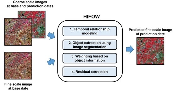
The first issue is of great importance for crop field monitoring at a fine scale, and the last two issues are associated with the extraction of temporal change information in crop fields. To this end, a four-step weighted function-based approach is adopted in HIFOW to create prediction results satisfying the above three issues. Methodological developments and the potential of HIFOW are demonstrated through STIF experiments on blending Sentinel-2 and RapidEye images at two agricultural sites.

2. Methods

As shown in Figure 1, HIFOW consists of four analytical steps: (1) temporal relationship modeling (hereafter referred to as TM), (2) object extraction using image segmentation, (3) weighting based on object information (hereafter referred to as WO), and (4) residual correction. The detailed explanations of each processing step are given as follows:

2.1. Temporal Relationship Modeling (TM)

In this step, a coarse-scale temporal relationship between FTCS images obtained at base and prediction dates is first estimated through local linear regression modeling. This step is employed to estimate temporal variability in spectral reflectance between the base and prediction dates.

Let $t_0$ and $t_p$ be the base date and the prediction date, respectively. In addition, suppose that $C\left(X, b_n,t_0\right)$ and $C\left(X, b_n,t_p\right)$ are the reflectance in the nth spectral band ($b_n$) of a coarse-scale pixel with its centroid $X$ of the FTCS imagery at $t_0$ and $t_p$, respectively. This study considers a local regression model to quantify local variability instead of a global regression model [33]. The local regression model, which uses $C\left(X, b_n,t_0\right)$ and $C\left(X, b_n,t_p\right)$ as an independent variable and a dependent variable, respectively, is fitted within the local window:

$$C\left(X, b_n,t_p\right)=a_0\left(X, b_n\right)+a_1\left(X, b_n\right)C\left(X, b_n,t_0\right)+R\left(X, b_n\right),$$

(1)

where $a_0\left(X, b_n\right)$ and $a_1\left(X, b_n\right)$ are two regression coefficients for the intercept and slope within the local window, respectively. $R\left(X, b_n\right)$ is the residual at a coarse scale that cannot be explained by the independent variable.

The linear relationship between the CTFS images modeled using Equation (1) is then applied to the CTFS imagery at $t_0$. Let $F\left(x, b_n,t_0\right)$ be the fine-scale CTFS imagery at any fine-scale pixel $x$ in the spectral band $b_k$ at $t_0$, where $x$ is located within the coarse-scale pixel $X$. Then, the initial prediction at $t_p$ (${\widehat{F}}_{TM}\left(x, b_n,t_p\right)$, hereafter referred to as the TM prediction) is obtained by applying the regression coefficients estimated from Equation (1):

$${\widehat{F}}_{TM}\left(x, b_n,t_p\right)=a_0\left(X, b_n\right)+a_1\left(X, b_n\right)F\left(x, b_n,t_0\right),$$

(2)

where all fine-scale pixels within any coarse-scale pixel ($x\in X$) share the same regression coefficients.

2.2. Object Extraction Using Image Segmentation

As a milestone of HIFOW, quantitative information of objects extracted through image segmentation using all available images is extracted in the second step to account for the characteristics of fine-scale images. More specifically, two image segmentation procedures using different inputs were designed to not only extract change information but also reflect spatial structures at a fine scale. First, multi-temporal image segmentation was presented to detect any temporal and structural changes from $t_0$ to $t_p$ within the study area. Second, fine-scale objects are also extracted from the CTFS imagery at $t_0$ to reflect the shape or structure at a fine scale in the prediction result.

The object-based approach is promising for STIF in small-scale croplands in that boundaries between crop fields and detailed spatial patterns within crop fields can be preserved by assigning a different weight per object, unlike the pixel-based approach in the existing STIF models. In this study, the multi-resolution segmentation approach [34] was applied to extract objects from input images.

As the first object extraction procedure, this study newly presents multi-temporal segmentation using two images at different dates as inputs to highlight changed objects with temporal variations in reflectance between the base and prediction dates. To this end, multi-spectral bands of the FTCS images at $t_0$ and $t_p$ are used sequentially as inputs for multi-resolution segmentation.

The multi-temporal segmentation approach for object-based change detection is illustrated in Figure 2. Suppose that two objects, A and B, called super-level objects, have been extracted from the FTCS imagery at $t_0$(Figure 2a). In the multi-temporal segmentation approach, further object extraction proceeds using the FTCS imagery at $t_p$ and the boundary information from the first segmentation result. Using the boundaries between A and B as supplementary information enables any object in the FTCS imagery at $t_0$ to be divided into other sub-level objects in the FTCS imagery at $t_p$ (i.e., B1 and B2 in Figure 2b) while preserving the object boundaries at $t_0$. Significant changes in reflectance of the FTCS imagery at $t_p$ result in the further sub-division of any super-level object at $t_0$. These sub-level objects can be regarded as objects, including spectral and structural changes between $t_0$ and $t_p$. Meanwhile, if the boundary or shape of any super-level object (i.e., A in Figure 2b) does not change, it can be considered that the object has no significant reflectance change that causes a change in shape or structure from $t_0$ to $t_p$. Such objects are regarded as non-changed ones. After binary labeling of the changed and non-changed objects (Figure 2c), the label information on temporal changes is used to assign different weights to changed and non-changed objects in step 3.

The objects at a fine scale are further extracted through image segmentation using the CTFS imagery at $t_0$ to obtain fine-scale structural information. The structural information includes boundaries between objects with different spectral responses within the same land-cover type, as well as boundaries between different land-cover types. Since pixels within a specific object are likely to have similar spectral reflectance, the object boundary information at a fine scale can be used to extract pixels with spectral similarity for determining weights in the third step of HIFOW.

2.3. Weighting Based on Object Information (WO)

In the third step, a specific procedure is presented that determines the weight fully reflecting temporal variations in reflectance. The key idea in step 3 is to determine the weight that not only complements the partial temporal change information from the TM prediction but also reflects the spectral patterns of the FTCS imagery at $t_p$. If the weight is assigned solely to one information source (i.e., the TM prediction or the FTCS imagery at $t_p$), the characteristics of images acquired at both $t_0$ and $t_p$ cannot be fully reflected in the prediction result. Therefore, it is reasonable to consider the weight to be applied to all the available information sources, including the TM prediction and the FTCS imagery at $t_p$. However, the two sources of information on temporal change have differing levels of richness of change information. Thus, the weight inter-connected by the relative importance of the two information sources is determined to fully utilize the available data.

To reflect the temporal variability in the weight, the absolute difference in reflectance between FTCS images at $t_0$ and $t_p$ is used as a measure of temporal change. The absolute difference measures the magnitude of the temporal change. Since only FTCS images are available at $t_0$ and $t_p$, it is not feasible to calculate the difference at a fine scale. Thus, the approximate absolute temporal difference is measured from the FTCS imagery resampled to the fine scale. Furthermore, the spatial context is considered to determine the weight based on the temporal difference. The spatial contextual information can be accounted for by quantifying the contribution of neighboring pixels using the fine-scale object information in step 2. To this end, a local search neighborhood centered at each fine-scale pixel is first set up to calculate the contributions from neighboring pixels for the weight determination. Pixels belonging to the same fine-scale object as the central pixel are selected as the neighboring ones within the search neighborhood. This selection procedure is considered because any pixels within the same object are likely to be spectrally similar and have the same land-cover type.

As a measure of temporal variability, the local temporal difference index (D) within the search neighborhood is defined as:

$$D\left(x_k, b_n\right)=\left| C_F\left(x_k, b_n,t_p\right)-C_F\left(x_k, b_n,t_0\right)\right|,$$

(3)

where $C_F$ is the FTCS imagery resampled to the fine scale. $x_k$ denotes the locations of the selected neighboring pixels within the predefined local search neighborhood centered at $x$.

As different land-cover types are likely to exhibit different temporal variability, D in Equation (3) is further normalized using the maximum value to adjust the range of the D values. The weight at $x$ is then calculated as the average of normalized D values within the search neighborhood as:

$$w\left(x, b_n\right)=\frac{1}{K}{{\displaystyle \sum }}_{k=0}^K\frac{D\left(x_k, b_n\right)}{D_{max}},$$

(4)

where $K$ and $D_{max}$ are the number of selected neighboring pixels and the maximum D value within the search neighborhood, respectively.

As the weight $w$ in Equation (4) directly reflects the temporal difference between $t_0$ and $t_p$, it is further used to impose the relative importance between the TM prediction and the FTCS imagery at $t_p$. As for the criterion for determining the relative importance using a single weight value $w$, this study assigns different weights to changed and non-changed objects extracted from multi-temporal segmentation in step 2. The TM prediction can account for the temporal variability of pixels with fewer temporal changes. On the other hand, the temporal variability of significantly changed pixels can be better explained by the FTCS imagery at $t_p$ than by the TM prediction. Thus, the importance of the FTCS imagery at $t_p$ is relatively more significant than that of the TM prediction, which does not have enough information at $t_p$. In contrast, more weight should be assigned to the TM prediction for any pixel within non-changed objects because the temporal variability is sufficiently explained by the TM prediction.

Based on the above relative importance of temporal changes, the prediction (${\widehat{F}}_{WO}$) in step 3 is defined as the different weighted sum of changed and non-changed objects:

$${\widehat{F}}_{WO}\left(x, b_n,t_p\right)=\left\{\begin{array}{cc}\left(1-w\left(x, b_n\right)\right){\widehat{F}}_{TM}\left(x, b_n,t_p\right)+w\left(x, b_n\right)C_F\left(x, b_n,t_p\right)& \mathrm{if} x\in O_{C } \\ w\left(x, b_n\right){\widehat{F}}_{TM}\left(x, b_n,t_p\right)+\left(1-w\left(x, b_n\right)\right)C_F\left(x, b_n,t_p\right)& \mathrm{if} x\in O_{NC}\end{array}\right.,$$

(5)

where $O_{C }$ and $O_{NC }$ are the changed and non-changed objects labeled in step 2. Hereafter, ${\widehat{F}}_{WO}$ is referred to as the WO prediction.

2.4. Residual Correction

The WO prediction obtained in step 3 may contain smoothed or blurred phenomena through the weighted combination procedure. Thus, improvement in the WO prediction is required to mitigate the blurring effects. In addition, there remain residuals after the regression modeling in step 1. The residuals indicate the components that cannot be accounted for by independent variables. In the first step, the FTCS imagery at $t_0$ is used as the independent variable to account for the spectral variability of the FTCS imagery at $t_p$. As a result, the residuals may contain temporal variation not modeled with regression. Thus, the residual correction can provide supplementary information, thereby improving the quality of the WO prediction.

As the residual correction requires the residuals at a fine scale, the coarse-scale residuals in Equation (1) should be spatially downscaled. In this study, as a simple but efficient downscaling method, a spline interpolator widely applied to the spatial downscaling of raster data [35,36] is employed for the residual downscaling.

The final HIFOW prediction (${\widehat{F}}_{HIFOW}$), which is considered the FST imagery, is generated by adding the fine-scale residuals to the WO prediction in step 3:

$${\widehat{F}}_{HIFOW}\left(x, b_n,t_p\right)={\widehat{F}}_{WO}\left(x, b_n,t_p\right)+\widehat{R}\left(x, b_n\right),$$

(6)

where $\widehat{R}\left(x, b_n\right)$ is the fine-scale residual at $x$ estimated by the spline interpolator.

3. Materials and Experimental Setup

3.1. Study Areas

Experiments were conducted at two agricultural sites in Korea, Hapcheon (Site 1) and Haenam (Site 2), to evaluate the practicability of HIFOW (Figure 3). The two agricultural sites were selected because phenological changes in crops and structural changes in fields are distinct, and crops are grown in small-scale fields. The availability of multi-temporal cloud-free images is usually limited in Korea. Hence, when the cloud-free regions were first extracted, the area covered by the two sites was relatively small. The total areas of the two sites are 676 ha and 1156 ha, respectively.

Site 1 includes small crop fields where garlic and onions are mainly grown, as well as small reservoirs and built-up areas. Paddy rice fields are the primary land-cover type of Site 2. Some grasslands within unmanaged paddy fields and parts of lakes also exist at Site 2. Site 2 is also covered with cabbage fields and barren lands in the northeastern and eastern parts. As shown in Figure 3, spatial heterogeneity between the two sites is quite different. The crop field size at Site 2 is relatively larger than that at Site 1. When class homogeneity is calculated as an indicator of the landscape homogeneity [37], class homogeneity for Site 1 is 0.78 with a standard deviation value of 0.22. In contrast, Site 2 has a class homogeneity value of 0.85 with a standard deviation value of 0.2, which indicates Site 1 is more heterogeneous than Site 2. Thus, the two sites were adequate for the comparative study.

3.2. Satellite Images

Sentinel-2 images with a spatial resolution of 10 m and 20 m and RapidEye images with a spatial resolution of 5 m were used as inputs for the STIF experiments (

Table 1. Summary of Sentinel-2 and RapidEye images used for the experiments.

Specification		Sentinel-2	RapidEye
Product type		Ortho Level-1C	Ortho Level-3A
Spatial resolution		10 m (Green, Red, NIR 1) 20 m (Red-edge)	5 m
Spectral band (Central wavelength)		Green (560 nm) Red (665 nm) Red-edge (705 nm) NIR 1 (842 nm)	Green (555 nm) Red (658 nm) Red-edge (710 nm) NIR 1 (805 nm)
Acquisition date	$t_0$2 (Site 1)	14 March 2018	12 March 2018
	$t_p$3 (Site 1)	10 May 2018	10 May 2018
	$t_0$2 (Site 2)	2 June 2019	4 June 2019
	$t_p$3 (Site 2)	10 October 2019	9 October 2019

¹ near infrared, ² base date, and ³ prediction date.

). The two satellite images were selected because they have the appropriate spatial resolution for monitoring small-scale crop fields and also have similar spectral bands, including the red-edge band.

In this study, the Sentinel-2 imagery was regarded as the FTCS imagery. The Sentinel-2 mission provides land surface imagery every 5 days through a combined constellation of two Sentinel-2 satellites (Sentinel-2A and -2B) [38]. Four spectral bands, including green, red, red-edge, and near-infrared (NIR) bands, were used for the experiments because they provide useful information for vegetation monitoring. Out of the four red-edge bands, band 5, with a central wavelength of 705 nm, was selected because its central wavelength is similar to that of the red-edge band of RapidEye imagery (710 nm). The Sentinel-2 reflectance products covering the study sites were downloaded from the Copernicus Open Access Hub [39].

The RapidEye is a constellation of five identical satellites, allowing image acquisition at a maximum of 5.5-day intervals, even though the revisit cycle of each satellite is 28 days [40]. Each RapidEye satellite has a swath width of approximately 77 km, capturing a relatively narrow range of images compared with the Sentinel-2 imagery (290 km). If the study area of interest is not in the path of the five satellites, the image acquisition day is likely to be more than the ideal 5.5 days. Thus, the RapidEye imagery with a spatial resolution of 5 m was considered as the CTFS imagery for STIF. As the input images for STIF should have the same physical quantity [28,41,42], the level-3A products were converted to reflectance [43], as with the Sentinel-2 imagery.

By considering the growth cycles of garlic and onions mainly grown in Site 1, two images acquired in March (growing stage) and May (harvesting stage) were selected as inputs for STIF. In the case of Site 2, two images acquired in June (growing stage) and October (harvesting stage) were also used as inputs for STIF. It should be noted that the spectral change in vegetation between $t_0$ and $t_p$ is significant in both study sites, which makes it suitable to evaluate the ability of HIFOW to depict temporal variability in spectral reflectance in the prediction result. As shown in Table 1, not all cloud-free Sentinel-2 and RapidEye images used in the experiment were obtained on the same date; however, the images acquired on a similar date were considered as pair images due to their similar spectral patterns. The RapidEye image at $t_p$ was assumed to be unavailable for STIF and used as the test data for computation of accuracy statistics.

Several preprocessing procedures were implemented using ENVI software version 5.6 (L3Harris Technologies, Broomfield, CO, USA), including geometric correction with digital topographic maps and sub-setting. When FTCS images (i.e., Sentinel-2 images in this study) need to be converted to a fine scale, we applied bilinear resampling, which has been widely applied in existing STIF studies.

3.3. Parameter Settings for HIFOW

The size of the local neighborhood used for both local regression modeling in step 1 and computation of the local temporal difference index in step 3 was set to five by considering the difference in spatial resolution between Sentinel-2 and RapidEye images as well as the size and distribution of crop fields.

eCognition [44] was utilized for the multi-resolution segmentation of multi-spectral images in step 2. In image segmentation, the optimal values of the scale parameter and the weights for color and shape were set through visual inspection of segmentation results. After examining the different scale parameter values from 50 to 200 with an interval of 10, the optimal scale parameter was set to 100 by visual inspection so that objects of smaller sizes could be generated. With respect to the weights for color and shape, the search range was set from 0.1 to 0.9 with an interval of 0.1. The criteria for selecting optimal weights for color and shape were differently applied to two image segmentation procedures. In multi-temporal segmentation, it is essential to capture changed objects with significant reflectance changes between $t_0$ and $t_p$. Thus, more importance was given to color. The weights for color and shape for multi-temporal segmentation were set to 0.8 and 0.2, respectively. Meanwhile, more weight was assigned to the shape because segmentation using the RapidEye image at $t_0$ aims to extract the structural information at a fine scale. Finally, 0.4 and 0.6 were selected as the optimal weights for color and shape, respectively.

3.4. Comparison and Evaluation

The interim prediction results of individual steps (i.e., TM prediction vs. WO prediction vs. final prediction) were first compared before evaluating the practicability of HIFOW with the existing STIF models. These comparisons can highlight the evolution of prediction results for each processing step and also confirm the effectiveness of individual steps of HIFOW.

The predictive performance of HIFOW was compared with three existing STIF models, including the spatial and temporal adaptive reflectance fusion model (STARFM), flexible spatiotemporal data fusion (FSDAF), and regression model fitting, spatial filtering, and residual compensation (Fit-FC). The three existing STIF models were chosen based on the following reasons: (1) they utilize a single image pair as input data, as in HIFOW, (2) they include the weight determination or local filtering step based on the local neighborhood system, and (3) their source code is publicly available [45,46,47]. For a fair comparison, the size of the local neighborhood or moving window, which is a parameter common to all three models, was set to 5, the same size applied to HIFOW. The number of neighboring pixels that are spectrally similar to the central pixel within the local neighborhood was set to 10 in consideration of the local neighborhood size. Moreover, the minimum number of land-cover classes required for FSDAF was set to 7, corresponding to the number of land-cover types in the two study sites.

The normalized difference vegetation index (NDVI), one of the representative vegetation indices [48,49], was further predicted to illustrate the practicability of HIFOW. The comparison of NDVI prediction was conducted because the two study sites mainly contain vegetation areas, such as crop fields. The NDVI may be calculated from the predicted reflectance values of the red and NIR bands. Such a blend-then-index approach is inevitably affected by errors attached to the prediction of reflectance. Thus, an index-then-blend approach, where the NDVI values calculated from each sensor image are directly fed into the STIF model, is preferred to mitigate error propagation problems [50]. In this study, the index-then-blend approach was employed for the prediction of NDVI.

For the quantitative assessment of prediction performance, accuracy statistics were computed by comparing the prediction results with the RapidEye image at $t_p$ that was not used for STIF. The root mean square error (RMSE) and the correlation coefficient (CC) were computed as quantitative accuracy measures. The relative RMSE (rRMSE) was also computed to consider the different ranges of individual spectral reflectance values. Given the actual RapidEye imagery ($F(x$)) and the predicted result ($\widehat{F}(x$)), the RMSE, rRMSE, and CC are calculated as:

$$\mathrm{RMSE}=\sqrt{\frac{1}{L}{\displaystyle \sum }_{l=1}^L{\left(\widehat{F}\left(x_l\right)-F\left(x_l\right)\right)}^2},$$

(7)

$$\mathrm{rRMSE}=\frac{\mathrm{RMSE}}{\mu },$$

(8)

$$\mathrm{CC}=\frac{\frac{1}{L}{{\displaystyle \sum }}_{l=1}^L\left(F\left(x_l\right)-\mu \right)\left(\widehat{F}\left(x_l\right)-\widehat{\mu }\right)}{\mathsf{\sigma } \mathsf{\sigma } ^},$$

(9)

where L is the total number of pixels. $\mu$ and $\mathsf{\sigma }$ are the mean and standard deviation values for the actual imagery, respectively. $\widehat{\mu }$ and $\mathsf{\sigma } ^$ are the mean and standard deviation values for the predicted imagery, respectively.

The relative improvement index (RI) was also computed to compare RMSE for HIFOW with other STIF models. The RI in the RMSE of HIFOW over a certain STIF model is defined as:

$$\mathrm{RI}\left(\%\right)=\frac{{\mathrm{RMSE}}_M-{\mathrm{RMSE}}_{\mathrm{HIFOW}}}{{\mathrm{RMSE}}_M}\times 100,$$

(10)

where ${\mathrm{RMSE}}_{\mathrm{HIFOW}}$ and ${\mathrm{RMSE}}_M$ denote the RMSE values of HIFOW and the specific STIF model M, respectively.

In addition to the above accuracy measures, the structural similarity (SSIM) was computed to measure the spatial similarity between actual RapidEye imagery and the prediction result [51]:

$$\mathrm{SSIM}=\frac{\left(2\mu \widehat{\mu }+c_1\right)\left(2\mathrm{Cov}+c_2\right)}{\left({\mu }^2+{\widehat{\mu }}^2+c_1\right)\left({\mathsf{\sigma }}^2+{ \mathsf{\sigma } ^}^2+c_2\right)},$$

(11)

where Cov denotes the covariance between the actual RapidEye imagery and the predicted result (i.e., the numerator in Equation (9)). $c_1$ and $c_2$ are two constants to avoid the division instability. SSIM ranges between zero and one, and its ideal value is one. The closer the SSIM value is to one, the better the prediction results represent the structure of the actual RapidEye imagery.

4. Results

4.1. Comparison between Interim Results of HIFOW

Figure 4 shows the multi-temporal segmentation results obtained from step 2 in a certain sub-area of Site 2 for illustration purposes. Figure 4a exhibits the object boundaries extracted from the Sentinel-2 imagery at $t_0$. The segmentation result for the Sentinel-2 imagery at $t_p$ in Figure 4b contains some objects further divided into sub-level objects while preserving the object boundary at $t_0$. The sub-level objects indicate that they experienced substantial changes in reflectance between $t_0$ and $t_p$, which can be regarded as changed objects, as shown in Figure 4c. Thus, the use of the object boundaries from the image at $t_0$ as constraint for image segmentation at $t_p$ enabled changed sub-areas to be highlighted as a single object.

Table 2. Band-wise accuracy statistics of interim prediction results of HIFOW on the two study sites. The best case is shown in bold.

Statistics	Band	Site 1			Site 2
		TM 1 Prediction	WO 2 Prediction	HIFOW 3 Prediction	TM 1 Prediction	WO 2 Prediction	HIFOW 3 Prediction
RMSE 4	Green	0.0098	0.0199	0.0054	0.0195	0.0166	0.0165
	Red	0.0169	0.0120	0.0089	0.0235	0.0175	0.0174
	Red-edge	0.0208	0.0298	0.0187	0.0195	0.0159	0.0167
	NIR	0.0270	0.0182	0.0152	0.0379	0.0290	0.0285
rRMSE 5	Green	0.0787	0.1590	0.0433	0.1942	0.1647	0.1643
	Red	0.1357	0.0958	0.0714	0.2330	0.1735	0.1726
	Red-edge	0.1668	0.2387	0.1500	0.1935	0.1578	0.1658
	NIR	0.2160	0.1455	0.1220	0.3762	0.2883	0.2833
CC 6	Green	0.8206	0.7277	0.9549	0.7571	0.8755	0.8830
	Red	0.7909	0.9050	0.9572	0.7103	0.8450	0.8604
	Red-edge	0.5470	0.8124	0.7646	0.8256	0.8780	0.8831
	NIR	0.8980	0.9607	0.9815	0.9037	0.9477	0.9548
SSIM 7	Green	0.8477	0.7631	0.9605	0.8352	0.8741	0.9453
	Red	0.8099	0.9137	0.9604	0.8394	0.8855	0.9453
	Red-edge	0.6087	0.8438	0.7920	0.7486	0.7766	0.9239
	NIR	0.9010	0.9618	0.9819	0.8614	0.9076	0.9599

¹ temporal relationship modeling, ² weighting based on object information,³ high spatial resolution image fusion using object-based weighting, ⁴ root mean square error, ⁵ relative root mean square error, ⁶ correlation coefficient, and ⁷ structural similarity.

lists the accuracy statistics of the interim results by individual steps of HIFOW. The HIFOW prediction showed superior prediction performance at both study sites. As analysis steps were applied sequentially, the predictive performance improved accordingly, except for green and red-edge bands at Site 1. The CC of the WO prediction for the red-edge band was higher than that of the HIFOW prediction; however, the HIFOW prediction still yielded the best RMSE and rRMSE.

Similar results were also obtained at Site 2. The RMSE and CC of the WO prediction were significantly improved by approximately 20% and 11%, respectively, compared with the TM prediction. The significant differences in RMSE and CC between the WO and HIFOW predictions were not observed. However, the increase in SSIM was prominent in the HIFOW prediction. The residuals retaining the overall structural information within the Sentinel-2 imagery at $t_p$ could increase the SSIM value through the residual correction.

In addition, the improvement in the prediction performance by the sequential applications of individual steps was more pronounced at Site 1 than at Site 2. As Site 1 is more locally heterogeneous than Site 2, this result demonstrates the effectiveness of the sequential application of individual steps of HIFOW for heterogeneous landscapes.

Figure 5 represents the interim results with the actual RapidEye imagery at Site 2, where one sub-area is also zoomed in for visual comparison. The TM prediction failed to produce spectral patterns consistent with the actual RapidEye imagery in several sub-areas. This spectral distortion is mainly due to the temporal variability of spectral reflectance between $t_0$ and $t_p$. As the June imagery was used as the independent variable in the regression modeling of step 1, such a temporal variability could not be well captured in the TM prediction. Meanwhile, the spectral distortion decreased by applying steps 3 and 4.

In the zoomed images, it is clearly seen that spatial details, including a specific spatial pattern inside the crop field, were lost in the TM prediction. On the contrary, many spatial details were reproduced in the WO predictions. The weighted combination using object information in step 3 significantly decreased the spectral distortion near the field boundary in the TM prediction. The relatively clearly captured boundaries of crop fields resulted from the use of object information from the RapidEye imagery at $t_0$. The residual correction created many enhanced spatial patterns in the HIFOW prediction. These detailed spatial patterns confirm the improved accuracy statistics of the HIFOW predictions in Table 2.

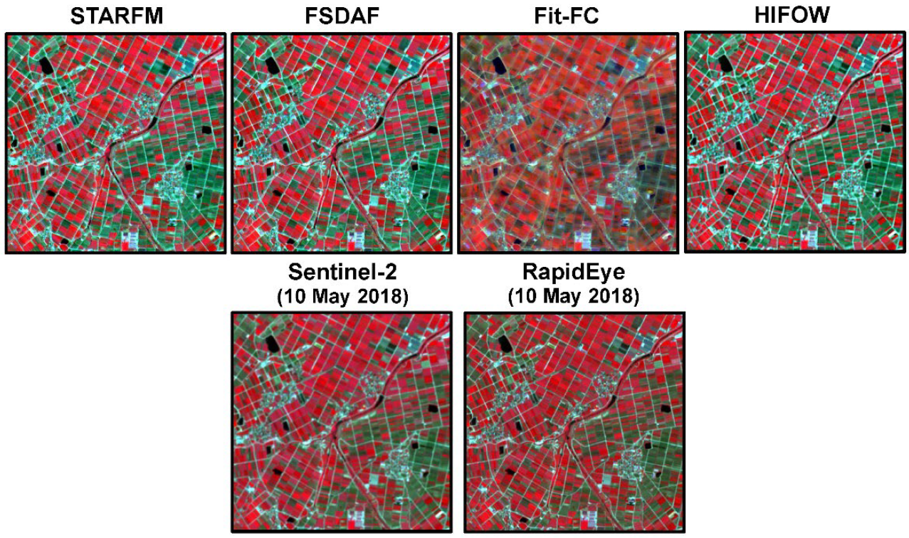
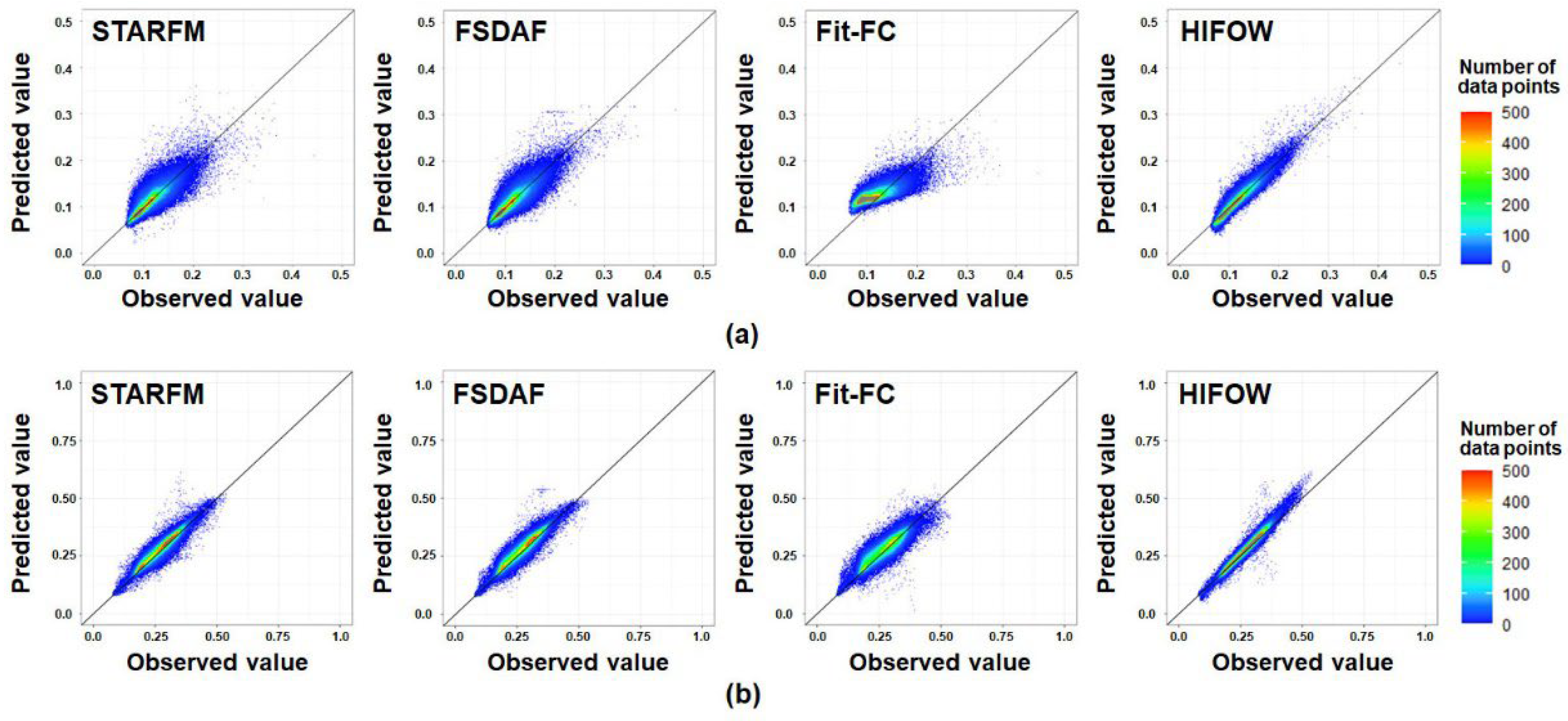
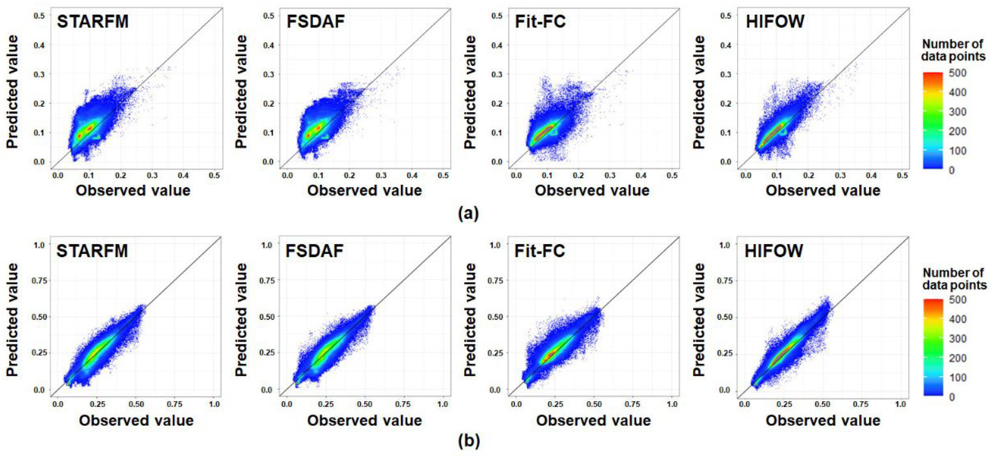
4.2. Comparison with other STIF Models

Figure 6 shows the prediction results of different STIF models at Site 1. The barren lands in the eastern part of the study site appeared brighter than the actual RapidEye imagery, whereas their spectral patterns were predicted to be darker by Fit-FC. Moreover, most spectral patterns of Fit-FC were spatially blurred and not consistent with the actual RapidEye imagery. Consequently, it is expected that Fit-FC would yield the worst RMSE and SSIM.

No apparent differences between the prediction results of HIFOW and the other two models were observed at Site 1 from the visual comparison. However, their differences are clearly shown at Site 2 (Figure 7). The prediction results of STARFM and FSDAF were very similar, with the greenish color (i.e., very low spectral reflectance in the NIR band) for grasslands grown in central unmanaged paddy fields. This result is mainly due to the strong effects of the RapidEye image at $t_0$. As shown in Figure 3, relatively low spectral reflectance in the NIR band in June was observed in these fields where the land-cover type was barren in June. As the land-cover type was changed to grassland in October, STARFM and FSDAF could not depict the spectral pattern at $t_p$. On the other hand, the prediction result of Fit-FC represented the temporal change in the reflectance of grassland well. However, the blurred boundaries of some cabbage fields in the northern and northeastern parts of the study area were observed in the Fit-FC prediction. Meanwhile, HIFOW produced the prediction results where the color was similar to the actual RapidEye image, except for some grassland fields with low reflectance in the NIR band.

The differences between the prediction results of the four STIF models are more clearly highlighted in some zoomed-in sub-areas (Figure 8). The results of STARFM and FSDAF at Site 1 contained spatially degraded boundaries and spectral distortions. In the FSDAF prediction, some artifacts were more pronounced than STARFM. The pixel-based classification contained in FSDAF may result in such artifacts. Severe spectral distortion was observed in the Fit-FC prediction (e.g., dark blue color patches in Figure 8). In contrast, blurred boundaries became more apparent, and the color and spatial details of the actual RapidEye image were well-represented in the HIFOW prediction.

Similar results were also obtained from Site 2. Similar to Site 1, STARFM and FSDAF produced similar prediction results with spectral distortion (e.g., light green field). Discontinuity of some pixels near the field boundary or inside the crop field was observed in the STARFM prediction. With respect to the Fit-FC prediction, the color tone was relatively similar to the actual RapidEye image, and the boundaries were clearly restored, compared with STARFM and FSDAF. However, there is still spectral distortion with isolated pixels due to salt and pepper effects. Moreover, spatial details inside the field were missing. Although a somewhat blurred prediction was obtained, HIFOW produced results with within-field details and spectral patterns similar to the actual image. The restoration of the fine-scale structures at $t_p$ could be achieved in the HIFOW prediction.

Table 3. Band-wise accuracy statistics of different STIF models at the two study sites. The best case is shown in bold.

Statistics	Band	Site 1				Site 2
		STARFM	FSDAF	Fit-FC	HIFOW	STARFM	FSDAF	Fit-FC	HIFOW
RMSE	Green	0.0084	0.0082	0.0170	0.0054	0.0248	0.0252	0.0188	0.0165
	Red	0.0140	0.0137	0.0229	0.0089	0.0300	0.0299	0.0215	0.0174
	Red edge	0.0192	0.0194	0.0206	0.0187	0.0230	0.0235	0.0238	0.0167
	NIR	0.0195	0.0218	0.0274	0.0152	0.0350	0.0356	0.0358	0.0285
rRMSE	Green	0.0673	0.0657	0.1361	0.0432	0.2461	0.2508	0.1872	0.1643
	Red	0.1121	0.1097	0.1833	0.0713	0.2982	0.2975	0.2140	0.1726
	Red edge	0.1537	0.1553	0.1649	0.1497	0.2285	0.2330	0.2360	0.1658
	NIR	0.1561	0.1745	0.2194	0.1217	0.3478	0.3535	0.3556	0.2833
CC	Green	0.8757	0.8880	0.6643	0.9549	0.6699	0.6434	0.7804	0.8830
	Red	0.8668	0.8748	0.7655	0.9572	0.6209	0.6151	0.7415	0.8604
	Red edge	0.6560	0.6521	0.6199	0.7646	0.7639	0.7437	0.7732	0.8831
	NIR	0.9551	0.9460	0.8943	0.9815	0.9188	0.9145	0.9110	0.9548
SSIM	Green	0.8929	0.9027	0.7115	0.9605	0.9139	0.8860	0.8658	0.9453
	Red	0.8777	0.8848	0.7985	0.9604	0.8900	0.8815	0.8731	0.9453
	Red edge	0.6972	0.6933	0.6667	0.7920	0.9027	0.8775	0.8665	0.9239
	NIR	0.9563	0.9475	0.8974	0.9819	0.9396	0.9267	0.8954	0.9599

reports quantitative assessment results for different STIF models. As expected, the accuracy statistics of HIFOW were consistent with the visual comparison results. HIFOW achieved the best prediction performance in terms of all accuracy statistics for both study sites. The RI in the RMSE of HIFOW is also listed in

Table 4. Relative improvement in RMSE of HIFOW over three STIF models at the two study sites (unit: %).

Band	Site1			Site2
	STARFM	FSDAF	Fit-FC	STARFM	FSDAF	Fit-FC
Green	35.7	34.1	68.2	33.2	34.5	12.2
Red	36.4	35.0	61.1	42.1	42.0	19.4
Red edge	2.6	3.6	9.2	27.4	28.8	29.7
NIR	22.1	30.3	44.5	18.5	19.9	20.3

. HIFOW improved the relative prediction accuracy from 2.6% to 68.2% at Site 1 and from 12.2% to 42.1% at Site 2. Furthermore, HIFOW exhibited much higher SSIM values than the other three models for all the spectral bands of both sites. The improvement in prediction accuracy of HIFOW was more significant in the green and red bands than in the red-edge and NIR bands. The relative improvement in prediction accuracy of HIFOW was not substantial for the red-edge band at Site 1. Meanwhile, the prediction performance of HIFOW for the red-edge band at Site 2 was much improved compared with Site 1. Except for the red-edge band, the relative improvement in RMSE of HIFOW over the other three models was much more pronounced at Site 1 than at Site 2, indicating the superiority of HIFOW for heterogeneous landscapes.

When comparing the prediction performance between the existing three models, the worst STIF model was Fit-FC in terms of RMSE, except for the green and red bands at Site 2. As expected from Figure 6–8, the SSIM of Fit-FC was the lowest for all spectral bands of both sites due to spatial blurring and severe spectral distortion. STARFM yielded the best RMSE for the red-edge and NIR bands at both sites and the highest SSIM for all spectral bands at Site 2. The RMSE and SSIM of FSDAF were better than those of STARFM and Fit-FC for the green and red bands at Site 1, whereas the RMSE of FSDAF was the worst for the green and red bands at Site 2.

The quantitative accuracy assessment results were further analyzed using the scatter-density plots of predicted values versus actual values in the red and NIR bands for individual models at both sites (Figure 9 and Figure 10). The two spectral bands were selected because they are usually utilized for the NDVI calculation.

With respect to Site 1, the data points of HIFOW were spread around the diagonal line and were more aggregated, consequently achieving a higher accuracy of HIFOW (Figure 9). The data points of STARFM and FSDAF were distributed similarly for both spectral bands; thus, the two models had similar RMSE values, as shown in Table 3. The noticeable result was obtained from the Fit-FC prediction for the red band. Most of the observation values of the red band from the actual RapidEye image are between 0.07 and 0.15. Fit-FC overestimated the values in this interval. Moreover, large values were seriously underestimated in the Fit-FC prediction. For the NIR band, the data points of the Fit-FC prediction exhibited greater dispersion and less aggregation, which led to the dark color in some crop fields, as shown in Figure 6. These unreliable predictions led to the poorest prediction performance of Fit-FC in terms of all the accuracy statistics. Some overestimated outliers, approximately 0.2 and 0.3 for the red and NIR bands, respectively, were observed in the HIFOW prediction. However, as these values were not too many and were scattered, their impact on the accuracy of statistics was insignificant.

With respect to Site 2, all STIF models presented more dispersion than Site 1 for two spectral bands (Figure 10). However, HIFOW still generated more aggregated predictions within the interval over which most actual values lie. Moreover, the data points of the HIFOW prediction fell closer to the diagonal line than those of other models. In particular, the dispersion was more severe for the red band than for the NIR band. The overestimation was observed for all models. Fit-FC and HIFOW presented more aggregation than STARFM and FSDAF. The greater density of Fit-FC and HIFOW for the NIR band was reflected in the central grassland fields. Consequently, the reflectance of the grassland was depicted well in the predictions of Fit-FC and HIFOW. The relatively low CC value of HIFOW for the red band in Table 3 resulted from scattered outliers around an actual value of 0.1.

4.3. NDVI Prediction Results

Figure 11 presents the accuracy assessment results of NDVI predictions using the index-then-blend approach. It reveals that HIFOW yielded the best prediction performance with the lowest RMSE, the largest CC, and the largest SSIM for both sites. Compared with STARFM, FSDAF, and Fit-FC, HIFOW increased the RMSE by 14.1–45.67% for Site 1 and 34.7–36.6% for Site 2. The RMSE of HIFOW at Site 1 was lower than that at Site 2 (0.0477 for Site 1 vs. 0.0736 for Site 2), and the SSIM of Site 1 was also greater than that of Site 2. The CC also showed almost similar results to the SSIM. Fit-FC was the poorest STIF model in the NDVI prediction, as well as in the prediction of reflectance.

Figure 12 illustrates the visual comparison results of NDVI predictions and absolute errors of different STIF models in the zoomed sub-area on Site 1. The other three models produced blurred results at the boundaries between crop fields and inside the crop fields. As a result, the absolute errors near the boundaries were greater than 0.2 for FSDAF and Fit-FC. In contrast, clear boundaries and consistent values within crop fields were restored in the HIFOW prediction. These results demonstrate the superiority of HIFOW for the prediction of NDVI and reflectance.

5. Discussion

5.1. Novelty of HIFOW

HIFOW was designed to consider three additional challenges associated with the STIF of high spatial resolution images, as mentioned in the introduction. All four steps of HIFOW are logically inter-linked within a unified framework. The TM prediction in step 1 is used as input for the weighted combination in step 3. The object extraction results in step 2 are also utilized in step 3. The residuals in step 1 and the OW prediction in step 3 are combined in step 4 to obtain a final prediction result.

Existing STIF models tend to generate prediction results greatly affected by the pair images at $t_0$. Thus, prediction performance is likely to decrease as the temporal distance or spectral variability between $t_0$ and $t_p$ becomes greater [31]. The acquisition of high spatial resolution images is often limited compared with coarse spatial resolution images. Thus, there is a great demand for effectively utilizing images acquired when $t_0$ and $t_p$ are temporally distant. As a solution to these limitations, HIFOW adopted the assumption that the temporal change in the FTCS imagery from $t_0$ to $t_p$ is also maintained in the CTFS imagery to reflect the change in spectral reflectance when the difference between image acquisition dates is great. This assumption was adopted because the temporal difference in spectral patterns is usually more influential than the difference in spectral patterns between the CTFS and FTCS images. STARFM also adopts this assumption for STIF. However, STARFM could not fully depict the spectral pattern at $t_p$ in this study when the difference in spectral reflectance between $t_0$ and $t_p$ was significant (Figure 6 and Figure 7). HIFOW could overcome the limitation through weighted combinations of information sources with different information richness for temporal variability. More weights were assigned to the spectral pattern from the resampled FTCS imagery at $t_p$ for changed objects, whereas more weights were assigned to the TM prediction in step 1 for non-changed objects. The latter weight assignment was implemented because only temporal differences in spectral reflectance need to be taken into account for non-changed objects. These different weighted combinations of complementary information based on the relative importance could generate a prediction result that reflects both temporal variability and spectral patterns at $t_p$.

The other novelty of HIFOW lies in the use of structural information in an object unit, not a pixel unit, which has great potential in blending fine-scale images. STARFM and Fit-FC consider the spatial contextual information by searching spectrally similar neighbor pixels, similar to HIFOW. However, the spatial contextual information is purely based on spectral reflectance in a pixel unit, which failed to fully represent meaningful spatial details in this study. On the other hand, the use of object-based information through image segmentation in HIFOW enabled reliable prediction of spatial details because any object belonging to the same land-cover type could be further divided into sub-level objects according to their spectral variability. As a result, HIFOW achieved the best SSIM values in both sites and better accuracy at Site 1 with more class heterogeneity than at Site 2 (Table 2, Table 3 and Table 4), which clearly demonstrates the benefit of using object-based information. This advantage can be more highlighted when fine-scale images are used for STIF in heterogeneous landscapes.

Although steps 2 and 3 are the key components of HIFOW, the application of residual correction as a final step also led to superior prediction performance, as shown in Table 2, which indicates that all four steps of HIFOW are essential to obtain satisfactory prediction results. The residuals from regression modeling contain two types of information: (1) temporal variability that regression modeling could not quantify and (2) spatial information in the FTCS imagery at $t_p$ that was not captured by the FTCS imagery at $t_0$. Due to the effect of the latter information, the residual correction notably led to a significant improvement in structural similarity. As the spatial resolution ratio between Sentinel-2 and RapidEye images is two for the green, red, and NIR bands, the contribution of the residual correction was more pronounced. As expected, the HIFOW prediction showed a lower SSIM on Site 1 and a larger RMSE on Site 2 for the red-edge band (Table 2). This result is mainly due to the relatively larger spatial resolution ratio of the red-edge band than the green, red, and NIR bands. Nevertheless, the HIFOW prediction achieved the best RMSE for the case with a lower SSIM on Site 1 and the best SSIM for the case with a lower RMSE on Site 2.

The superior accuracy of HIFOW over the other STIF models for the NDVI prediction further confirms its ability to blend other variables from multi-sensor remote sensing images with different resolutions, although extensive experiments are required for blending other variables besides reflectance and NDVI.

When visually comparing the HIFOW prediction with the Sentinel-2 image at $t_p$, spatial details of the images were depicted in the results, as well as the temporal change between $t_0$ and $t_p$, since HIFOW contains a procedure that explicitly accounts for the spectral pattern from the CTFS image at $t_p$. Other than this nature of HIFOW, structural change information is also considered through the weight determination based on the object information. Therefore, it is anticipated that HIFOW could be beneficial in detecting objects undergoing severe structural changes due to floods, wildfires, and landslides at a fine scale.

5.2. Future Research Directions

The performance of any STIF model is affected by several influential factors [52,53]. Despite its promising prediction performance, HIFOW does not have any procedure to correct radiometric inconsistency between multi-sensor images at $t_0$ caused by different sensor types and differences in image acquisition dates. Multi-sensor images have different bandwidths and spectral responses for the same spectral bands. For example, the RapidEye imagery has wider bandwidths than the Sentinel-2 imagery [54]. These different radiometric characteristics of multi-sensor images would affect the prediction performance of STIF. The HIFOW prediction contained the blurring phenomenon to some extent, which may result from the radiometric inconsistency between multi-sensor images. To alleviate the effects of radiometric inconsistency, radiometric normalization, or relative radiometric correction [54,55], should be considered as a preprocessing step of HIFOW.

Apart from the radiometric inconsistency, the spatial resolution ratio between coarse and fine images is one of the influential factors in STIF. The spatial resolution ratio of Sentinel-2 and RapidEye images used in this study is only two for the green, red, and NIR bands, or up to four for the red-edge band. The lower accuracy for the red-edge band mainly resulted from the relatively larger spatial resolution ratio between Sentinel-2 and RapidEye images. Zhou et al. [52] reported that the prediction performance generally worsens as the spatial resolution ratio increases. A similar result was found in our previous study [54], where blending Sentinel-2 and PlanetScope images yielded a worse prediction accuracy than blending Sentinel-2 and RapidEye images. The spatial resolution ratios of the former and latter cases were four and two, respectively. The considerable difference in spatial resolution tends to increase blocky artifacts in the prediction result, which cannot be fully alleviated by residual correction. This phenomenon was not observed in our experiments due to the small spatial resolution ratio. Moreover, HIFOW could alleviate the artifacts by adopting the object-based approach and considering the spatial context. Extensive experiments using multi-sensor images with different spatial resolution ratios should be performed to verify the robustness of HIFOW to the spatial resolution ratio.

Since the use of object-based information is one of the critical parts of HIFOW, the quality of segmentation results may affect the prediction performance. The segmentation quality usually depends on several factors, including segmentation algorithms and parameter settings. In this study, optimal parameters for image segmentation using eCognition were empirically determined via a trial-and-error approach, and the segmentation results were assessed by visual inspection. Instead of using multi-resolution image segmentation of commercial software, other segmentation algorithms (e.g., watershed-based clustering [56] and simple linear iterative clustering (SLIC) [57]) and freely available software or libraries (e.g., scikit-image [58]) can be applied to image segmentation. Thus, the influence of segmentation quality on prediction performance should be further assessed in future work.

Recently, Zhang et al. [59] presented an object-based STIF model with multi-resolution segmentation, linear injection, and spatial filtering. The object extraction and selection of spectrally similar pixels in their approach may be similar to HIFOW. However, HIFOW differs from their approach in that change information is directly extracted from multi-temporal image segmentation, and residual correction is further applied to complement temporal variations. As the availability of high spatial resolution satellite images increases, it is worth comparing the predictive performance of HIFOW with other STIF models developed for blending multi-sensor high spatial resolution images [32,59].

The main objective of this study was to develop an advanced STIF model for high spatial resolution satellite images. Thus, the fused FST images were not directly utilized to monitor the small-scale croplands via time-series analysis. STIF requires multi-sensor image pairs at $t_0$ and the FTCS imagery at $t_p$. The input images must be cloud-free. However, the availability of cloud-free fine spatial resolution images is much more limited than coarse or medium spatial resolution images because of their low temporal resolution. Thus, the limited availability of cloud-free fine spatial resolution satellite images is an obstacle to applying STIF models. This limitation from a data availability perspective can be overcome by combining STIF tasks with cloud removal or image reconstruction [60]. Future research will be directed toward the practical application of STIF combined with image reconstruction for crop field monitoring.

6. Conclusions

This paper presents a new STIF model, called HIFOW, to blend multi-sensor high spatial resolution satellite images for small-scale cropland monitoring. The four-step approach can not only quantify temporal variability between the base and prediction dates but also reflect structural information and spectral patterns at the prediction date. The prediction performance of HIFOW for STIF of high spatial resolution images was evaluated from experiments on two small agricultural sites using Sentinel-2 and RapidEye images. Compared with the existing STIF models, HIFOW achieved superior prediction performance for all spectral bands in terms of accuracy and structural similarity. HIFOW improved the relative prediction accuracy by up to 68.2% for Site 1 and 42.1% for Site 2 and exhibited the largest structural similarity value. Furthermore, HIFOW exhibited the lowest prediction accuracy (0.048 for Site 1 and 0.074 for Site 2) and the largest structural similarity (0.970 for Site 1 and 0.954 for Site 2) for the NDVI prediction. Object-based change and structural information obtained from image segmentation could facilitate reflecting detailed spatial features, such as field boundaries and specific patterns, with less spectral distortion in the HIFOW prediction. These results confirmed the feasibility of HIFOW to construct a time-series image set suitable for monitoring small-scale croplands.

References

1. Rogan, J.; Chen, D. Remote sensing technology for mapping and monitoring land-cover and land-use change. Prog. Plann. 2004, 61, 301–325. [Google Scholar] [CrossRef]
2. Maktav, D.; Erbek, F.S.; Jürgens, C. Remote sensing of urban areas. Int. J. Remote Sens. 2006, 26, 655–659. [Google Scholar] [CrossRef]
3. Ozdogan, M.; Yang, Y.; Allez, G.; Cervantes, C. Remote sensing of irrigated agriculture: Opportunities and challenges. Remote Sens. 2010, 2, 2274–2304. [Google Scholar] [CrossRef] [Green Version]
4. Muller-Karger, F.; Roffer, M.; Walker, N.; Oliver, M.; Schofield, O.; Abbott, M.; Graber, H.; Leben, R.; Goni, G. Satellite remote sensing in support of an integrated ocean observing system. IEEE Geosci. Remote Sens. Mag. 2013, 1, 8–18. [Google Scholar] [CrossRef]
5. Ryu, S.; Kwon, Y.-J.; Kim, G.; Hong, S. Temperature vegetation dryness index-based soil moisture retrieval algorithm developed for Geo-KOMPSAT-2A. Remote Sens. 2021, 13, 2990. [Google Scholar] [CrossRef]
6. Park, N.-W.; Kim, Y.; Kwak, G.-H. An overview of theoretical and practical issues in spatial downscaling of coarse resolution satellite-derived products. Korean J. Remote Sens. 2019, 35, 589–607. [Google Scholar]
7. Dawbin, K.W.; Evans, J.C. Large area crop classification in New South Wales, Australia, using Landsat data. Int. J. Remote Sens. 1988, 9, 295–301. [Google Scholar] [CrossRef]
8. Wardlow, B.D.; Egbert, S.L. Large-area crop mapping using time-series MODIS 250 m NDVI data: An assessment for the U.S. Central Great Plains. Remote Sens. Environ. 2008, 112, 1096–1116. [Google Scholar] [CrossRef]
9. Kussul, N.; Lemoine, G.; Gallego, F.J.; Skakun, S.V.; Lavreniuk, M.; Shelestov, A.Y. Parcel-based crop classification in Ukraine using Landsat-8 data and Sentinel-1A data. IEEE J. Sel. Top. Appl. Earth Obs. Remote Sens. 2016, 9, 2500–2508. [Google Scholar] [CrossRef]
10. Kim, Y.; Kyriakidis, P.C.; Park, N.-W. A cross-resolution, spatiotemporal geostatistical fusion model for combining satellite image time-series of different spatial and temporal resolutions. Remote Sens. 2020, 12, 1553. [Google Scholar] [CrossRef]
11. Cadastral Statistical Annual Report 2021. National Spatial Data Infrastructure Portal. Available online: https://nsdi.go.kr (accessed on 4 July 2022).
12. Zhang, H.; Li, Q.; Liu, J.; Shang, J.; Du, X.; McNairn, H.; Champagne, C.; Dong, T.; Liu, M. Image classification using RapidEye data: Integration of spectral and textual features in a random forest classifier. IEEE J. Sel. Top. Appl. Earth Obs. Remote Sens. 2017, 10, 5334–5349. [Google Scholar] [CrossRef]
13. Jin, Y.; Guo, J.; Ye, H.; Zhao, J.; Huang, W.; Cui, B. Extraction of arecanut planting distribution based on the feature space optimization of PlanetScope imagery. Agriculture 2021, 11, 371. [Google Scholar] [CrossRef]
14. Sagan, V.; Maimaitijiang, M.; Bhadra, S.; Maimaitiyiming, M.; Brown, D.R.; Sidike, P.; Fritschi, F.B. Field-scale crop yield prediction using multi-temporal WorldView-3 and PlanetScope satellite data and deep learning. ISPRS J. Photogramm. Remote Sens. 2021, 174, 265–281. [Google Scholar] [CrossRef]
15. Ghamisi, P.; Rasti, B.; Yokoya, N.; Wang, Q.; Höfle, B.; Bruzzone, L.; Bovolo, F.; Chi, M.; Anders, K.; Gloaguen, R.; et al. Multisource and multitemporal data fusion in remote sensing: A comprehensive review of the state of the art. IEEE Geosci. Remote Sens. Mag. 2019, 7, 6–39. [Google Scholar] [CrossRef] [Green Version]
16. Zhu, X.; Cai, F.; Tian, J.; Williams, T.K.-A. Spatiotemporal fusion of multisource remote sensing data: Literature survey, taxonomy, principles, applications, and future directions. Remote Sens. 2018, 10, 527. [Google Scholar] [CrossRef] [Green Version]
17. Belgiu, M.; Stein, A. Spatiotemporal image fusion in remote sensing. Remote Sens. 2019, 11, 818. [Google Scholar] [CrossRef] [Green Version]
18. Gao, F.; Masek, J.; Schwaller, M.; Hall, F. On the blending of the Landsat and MODIS surface reflectance: Predicting daily Landsat surface reflectance. IEEE Trans. Geosci. Remote Sens. 2006, 44, 2207–2218. [Google Scholar]
19. Zhu, X.; Chen, J.; Gao, F.; Chen, X.; Masek, J.G. An enhanced spatial and temporal adaptive reflectance fusion model for complex heterogeneous regions. Remote Sens. Environ. 2010, 114, 2610–2623. [Google Scholar] [CrossRef]
20. Wang, Q.; Atkinson, P.M. Spatio-temporal fusion for daily Sentinel-2 images. Remote Sens. Environ. 2018, 204, 31–42. [Google Scholar] [CrossRef] [Green Version]
21. Wu, M.; Niu, Z.; Wang, C.; Wu, C.; Wang, L. Use of MODIS and Landsat time series data to generate high-resolution temporal synthetic Landsat data using a spatial and temporal reflectance fusion model. J. App. Remote Sens. 2012, 6, 063507. [Google Scholar]
22. Gevaert, C.M.; García-Haro, F.J. A comparison of STARFM and an unmixing-based algorithm for Landsat and MODIS data fusion. Remote Sens. Environ. 2015, 156, 34–44. [Google Scholar] [CrossRef]
23. Huang, B.; Song, H. Spatiotemporal reflectance fusion via sparse representation. IEEE Trans. Geosci. Remote Sens. 2012, 50, 3707–3716. [Google Scholar] [CrossRef]
24. Song, H.; Huang, B. Spatiotemporal satellite image fusion through one-pair image learning. IEEE Trans. Geosci. Remote Sens. 2013, 51, 1883–1896. [Google Scholar] [CrossRef]
25. Tan, Z.; Yue, P.; Di, L.; Tang, J. Deriving high spatiotemporal remote sensing images using deep convolutional network. Remote Sens. 2018, 10, 1066. [Google Scholar] [CrossRef] [Green Version]
26. Jia, D.; Song, C.; Cheng, C.; Shen, S.; Ning, L.; Hui, C. A novel deep learning-based spatiotemporal fusion method for combining satellite images with different resolutions using a two-stream convolutional neural network. Remote Sens. 2020, 12, 698. [Google Scholar] [CrossRef] [Green Version]
27. Zhang, H.; Song, Y.; Han, C.; Zhang, L. Remote sensing image spatiotemporal fusion using a generative adversarial network. IEEE Trans. Geosci. Remote Sens. 2021, 59, 4273–4286. [Google Scholar] [CrossRef]
28. Zhu, X.; Helmer, E.H.; Gao, F.; Liu, D.; Chen, J.; Lefsky, M.A. A flexible spatiotemporal method for fusing satellite images with different resolutions. Remote Sens. Environ. 2016, 172, 165–177. [Google Scholar] [CrossRef]
29. Emelyanova, I.V.; McVicar, T.R.; Van Niel, T.G.; Li, L.T.; van Dijk, A.I.J.M. Assessing the accuracy of blending Landsat-MODIS surface reflectances in two landscapes with contrasting spatial and temporal dynamics: A framework for algorithm selection. Remote Sens. Environ. 2013, 133, 193–209. [Google Scholar] [CrossRef]
30. Chen, B.; Huang, B.; Xu, B. Comparison of spatiotemporal fusion models: A review. Remote Sens. 2015, 7, 1798–1835. [Google Scholar] [CrossRef] [Green Version]
31. Park, S.; Kim, Y.; Na, S.-I.; Park, N.-W. Evaluation of spatio-temporal fusion models of multi-sensor high-resolution satellite images for crop monitoring: An experiment on the fusion of Sentinel-2 and RapidEye images. Korean J. Remote Sens. 2020, 35, 807–821, (In Korean with English Abstract). [Google Scholar]
32. Jiang, J.; Zhang, Q.; Yao, X.; Tian, Y.; Zhu, Y.; Cao, W.; Cheng, T. HISTIF: A new spatiotemporal image fusion method for high-resolution monitoring of crops at the subfield level. IEEE J. Sel. Top. Appl. Earth Obs. Remote Sens. 2020, 13, 4607–4626. [Google Scholar] [CrossRef]
33. Kim, Y.; Park, N.-W. Impact of trend estimates on predictive performance in model evaluation for spatial downscaling of satellite-based precipitation data. Korean J. Remote Sens. 2017, 33, 25–35. [Google Scholar] [CrossRef] [Green Version]
34. Benz, U.C.; Hofmann, P.; Willhauck, G.; Lingenfelder, I.; Heynen, M. Multi-resolution, object-oriented fuzzy analysis of remote sensing data for GIS-ready information. ISPRS J. Photogramm. Remote Sens. 2004, 58, 239–258. [Google Scholar] [CrossRef]
35. Immerzeel, W.W.; Rutten, M.M.; Droogers, P. Spatial downscaling of TRMM precipitation using vegetative response on the Iberian Peninsula. Remote Sens. Environ. 2009, 113, 362–370. [Google Scholar] [CrossRef]
36. Sharifi, E.; Saghafian, B.; Steinacker, R. Downscaling satellite precipitation estimates with multiple linear regression, artificial neural networks, and spline interpolation techniques. J. Geophys. Res. Atmos. 2019, 124, 789–805. [Google Scholar] [CrossRef] [Green Version]
37. Park, S.; Park, N.-W. Effects of class purity of training patch on classification performance of crop classification with convolutional neural network. Appl. Sci. 2020, 10, 3773. [Google Scholar] [CrossRef]
38. Gascon, F.; Bouzinac, C.; Thépaut, O.; Jung, M.; Francesconi, B.; Louis, J.; Languille, F. Copernicus Sentinel-2A calibration and products validation status. Remote Sens. 2017, 9, 584. [Google Scholar] [CrossRef] [Green Version]
39. ESA, Copernicus Open Access Hub. Available online: https://scihub.copernicus.eu (accessed on 13 December 2021).
40. Tyc, G.; Tulip, J.; Schulten, D.; Krischke, M.; Oxfort, M. The RapidEye mission design. Acta Astronaut. 2005, 56, 213–219. [Google Scholar] [CrossRef]
41. Bai, B.; Tan, Y.; Donchyts, G.; Haag, A.; Weerts, A. A simple spatio–temporal data fusion method based on linear regression coefficient compensation. Remote Sens. 2020, 12, 3900. [Google Scholar] [CrossRef]
42. Wei, X.; Chang, N.B.; Bai, K. A comparative assessment of multisensor data merging and fusion algorithms for high-resolution surface reflectance data. IEEE J. Sel. Top. Appl. Earth Obs. Remote Sens. 2020, 13, 4044–4059. [Google Scholar] [CrossRef]
43. Chander, G.; Haque, M.O.; Sampath, A.; Brunn, A.; Trosset, G.; Hoffmann, D.; Anderson, C. Radiometric and geometric assessment of data from the RapidEye constellation of satellites. Int. J. Remote Sens. 2013, 34, 5905–5925. [Google Scholar] [CrossRef]
44. eCognition. Available online: https://geospatial.trimble.com/products-and-solutions/ecognition (accessed on 23 May 2022).
45. STARFM. Available online: https://www.ars.usda.gov/research/software/download/?softwareid=432 (accessed on 28 March 2022).
46. FSDAF. Available online: https://xiaolinzhu.weebly.com/open-source-code.html (accessed on 28 March 2022).
47. Fit-FC. Available online: https://github.com/qunmingwang/Fit-FC (accessed on 28 March 2022).
48. Maselli, F.; Chiesi, M.; Pieri, M. A new method to enhance the spatial features of multitemporal NDVI image series. IEEE Trans. Geosci. Remote Sens. 2019, 57, 4967–4979. [Google Scholar] [CrossRef]
49. Sun, R.; Chen, S.; Su, H.; Mi, C.; Jin, N. The effect of NDVI time series density derived from spatiotemporal fusion of multisource remote sensing data on crop classification accuracy. ISPRS Int. J. Geo.-Inf. 2019, 8, 502. [Google Scholar] [CrossRef] [Green Version]
50. Jarihani, A.A.; McVicar, T.R.; Van Niel, T.G.; Emelyanova, I.V.; Callow, J.N.; Johansen, K. Blending Landsat and MODIS data to generate multispectral indices: A comparison of “Index-then-Blend” and “Blend-then-Index” approaches. Remote Sens. 2014, 6, 9213–9238. [Google Scholar] [CrossRef]
51. Wang, Z.; Bovik, A.C.; Sheikh, H.R.; Simoncelli, E.P. Image quality assessment: From error visibility to structural similarity. IEEE Trans. Image Process. 2004, 13, 600–612. [Google Scholar] [CrossRef] [PubMed] [Green Version]
52. Zhou, J.; Chen, J.; Chen, X.; Zhu, X.; Qiu, Y.; Song, H.; Rao, Y.; Zhang, C.; Cao, X.; Cui, X. Sensitivity of six typical spatiotemporal fusion methods to different influential factors: A comparative study for a normalized difference vegetation index time series reconstruction. Remote Sens. Environ. 2021, 252, 112130. [Google Scholar] [CrossRef]
53. Liu, M.; Ke, Y.; Yin, Q.; Chen, X.; Im, J. Comparison of five spatio-temporal satellite image fusion models over landscapes with various spatial heterogeneity and temporal variation. Remote Sens. 2019, 11, 2612. [Google Scholar] [CrossRef] [Green Version]
54. Park, S.; Na, S.-I.; Park, N.-W. Effect of correcting radiometric inconsistency between input images on spatio-temporal fusion of multi-sensor high-resolution satellite images. Korean J. Remote Sens. 2021, 37, 999–1011, (In Korean with English Abstract). [Google Scholar]
55. Zhao, Y.; Huang, B.; Song, H. A robust adaptive spatial and temporal image fusion model for complex land surface changes. Remote Sens. Environ. 2018, 208, 42–62. [Google Scholar] [CrossRef]
56. Vincent, L.; Soille, P. Watersheds in digital spaces: An efficient algorithm based on immersion simulations. IEEE Trans. Pattern Anal. Mach. Intell. 1991, 13, 583–598. [Google Scholar] [CrossRef] [Green Version]
57. Achanta, R.; Shaji, A.; Smith, K.; Lucchi, A.; Fua, P.; Süsstrunk, S. SLIC superpixels compared to state-of-the-art superpixel methods. IEEE Trans. Pattern Anal. Mach. Intell. 2012, 34, 2274–2282. [Google Scholar] [CrossRef] [PubMed] [Green Version]
58. Scikit-Image: Image Processing in Python. Available online: https://scikit-image.org/docs/stable/api/skimage.segmentation.html (accessed on 13 September 2022).
59. Zhang, H.; Sun, Y.; Shi, W.; Guo, D.; Zheng, N. An object-based spatiotemporal fusion model for remote sensing images. Eur. J. Remote Sens. 2021, 54, 86–101. [Google Scholar] [CrossRef]
60. Shen, H.; Li, X.; Cheng, Q.; Zeng, C.; Yang, G.; Li, H.; Zhang, L. Missing information reconstruction of remote sensing data: A technical review. IEEE Geosci. Remote Sens. Mag. 2015, 3, 61–85. [Google Scholar] [CrossRef]
Figure 1. Schematic diagram of four processing steps employed in this study. Blocks in green denote the major steps of HIFOW.
Agronomy 12 02572 g001
Figure 2. Illustration of object-based change detection through multi-temporal segmentation: (a) Two objects, A and B, at the base date; (b) three objects, A, B1, and B2, at the prediction date, where object B at the base date is sub-divided into two objects, B1 and B2; (c) labeling of the changed and non-changed objects, where NC and C indicate the non-changed and changed objects, respectively.
Agronomy 12 02572 g002
Figure 3. Sentinel-2 and RapidEye color composite images at the two sites (NIR-red-green as RGB).
Agronomy 12 02572 g003
Figure 4. Illustration of multi-temporal segmentation results in the sub-area of Site 2. All color composite images are displayed with NIR-red-green as RGB: (a) Object boundaries superimposed on Sentinel-2 imagery at the base date (2 June 2018); (b) object boundaries superimposed on Sentinel-2 imagery at the prediction date (10 October 2018); and (c) changed objects highlighted in blue, where black polygons denote the objects boundaries in both (a,b).
Agronomy 12 02572 g004
Figure 5. Interim prediction results of HIFOW and actual RapidEye imagery at Site 2 (NIR-red-green as RGB). The black box marked in the first-row imagery is zoomed in the second row.
Agronomy 12 02572 g005
Figure 6. Prediction results of different STIF models with Sentinel-2 and RapidEye images at the prediction date (10 May 2018) at Site 1. All color composite images are displayed with NIR-red-green as RGB.
Agronomy 12 02572 g006
Figure 7. Prediction results of different STIF models with Sentinel-2 (10 October. 2019) and RapidEye images (9 October. 2019) at the prediction date at Site 2. All color composite images are displayed with NIR-red-green as RGB.
Agronomy 12 02572 g007
Figure 8. Prediction results of different STIF models with Sentinel-2 and RapidEye images in the zoomed-in sub-areas at the two sites. The sub-area marked with a white box in the Sentinel-2 imagery is enlarged. All color composite images are displayed with NIR-red-green as RGB.
Agronomy 12 02572 g008
Figure 9. Scatter-density plots of predicted values versus actual values for different STIF models on Site 1: (a) red band; (b) NIR band.
Agronomy 12 02572 g009
Figure 10. Scatter-density plots of predicted values versus actual values for different STIF models on Site 2: (a) red band; (b) NIR band.
Agronomy 12 02572 g010
Figure 11. Accuracy statistics of the NDVI prediction results for different STIF models at both sites: (a) RMSE; (b) CC; and (c) SSIM.
Agronomy 12 02572 g011
Figure 12. NDVI prediction results (first row) and absolute error distributions (second row) at the zoomed sub-area on Site 1. The sub-area marked with the black box in the left RapidEye NDVI image is enlarged.
Agronomy 12 02572 g012