Article

Smart Farm Irrigation: Model Predictive Control for Economic Optimal Irrigation in Agriculture

1
Departamento de Ingeniería, Universidad Loyola Andalucía, 41704 Dos Hermanas, Spain
2
IFAPA Centro de Alameda del Obispo, Junta de Andalucía, 14004 Córdoba, Spain
*
Author to whom correspondence should be addressed.
These authors contributed equally to this work.
Agronomy 2021, 11(9), 1810; https://doi.org/10.3390/agronomy11091810
Submission received: 2 August 2021 / Revised: 1 September 2021 / Accepted: 6 September 2021 / Published: 9 September 2021

Abstract

:
The growth of the global population, together with climate change and water scarcity, has made the shift towards efficient and sustainable agriculture increasingly important. Undoubtedly, the recent development of low-cost IoT-based sensors and actuators offers great opportunities in this direction since these devices can be easily deployed to implement advanced monitoring and irrigation control techniques at a farm scale, saving energy and water and decreasing costs. This paper proposes an economic and periodic predictive controller taking advantage of the irrigation periodicity. The goal of the controller is to find an irrigation technique that optimizes water and energy consumption while ensuring adequate levels of soil moisture for crops, achieving the maximum crop yield. For this purpose, the developed predictive controller makes use of soil moisture data at different depths, and it formulates a constrained optimization problem that considers energy and water costs, crop transpiration, and an accurate dynamical nonlinear model of the water dynamics in the soil, reflecting the reality. This controller strategy is compared with a classical irrigation strategy adopted by a human expert in a specific case study, demonstrating that it is possible to obtain significant reductions in water and energy consumption without compromising crop yields.

1. Introduction

Globally, agriculture is the largest consumer of water, accounting for approximately 70% of total water consumption, up to 80% in some areas [1]. Deficient water management is a huge concern, not only due to the depletion of the vital resource but also because over-irrigation results in the higher use of energy, loss of competitiveness, a reduction in crop productivity, and pollution of aquifers by fertilizers [2]. Consequently, policymakers in Europe are creating strategies to increase the sustainability of food production along with a complete value change, stressing the need for efficient management of water resources (see, for instance, the Farm to Fork Strategy [3] of the European Green Deal [4]).
Even in countries with a high degree of irrigation modernization, irrigation scheduling is based on the experience of farmers and/or technical advisors [5]. The variety of factors (weather, soil, crop, irrigation system, etc.) to take into account requires farmers’ dedication, perseverance, and expertise in implementing an optimized irrigation strategy [6]. In this context, the paradigm of precision sustainable irrigation now seems inexorably linked to digital tools and irrigation automation in order to alleviate the time and expertise requirements for farmers.
Recent advances in the Internet of Things (IoT) are based on the farm scale to increase crop productivity and water use efficiency while lowering energy costs and reducing the environmental footprint. The better performance of automated irrigation scheduling may be attributed to its faster response to changes in soil–plant–weather conditions, as well as its ability to self-tune the irrigation requirements according to the precise conditions of each plot. In addition, some studies concluded that no single sensor on its own will indicate the optimal amount of water applied, while mathematical methods, such as the control model, could help to identify and implement optimal irrigation management [7].
Automatized irrigation scheduling, based on the FAO’s water balance model and/or moisture sensors, has received significant research attention in the last few decades [8]. The approach of the FAO’s soil water balance is the most common method for calculating irrigation requirements, where the water inputs in the soil–plant system are compared with the outputs [9].
Based on science-driven techniques, simple and elaborated approaches have been used for optimizing irrigation through automatic irrigation controllers [6]. One of the simplest approaches is to set in the irrigation automata a conservative general irrigation program, an automated system that switches on/off the irrigation system whenever the soil moisture is below/above predetermined thresholds [10]. Another simple approach used in automated irrigation involves soil moisture sensors or tensiometers centered on initiating/terminating the irrigation when the measurements provided by the sensors rise above or fall below pre-established thresholds [11]. A more elaborate approach is to determine irrigation doses via the water balance, but using feedback from plant or soil sensors [8]. This combination of water balance and sensors demonstrates the ability to calculate irrigation doses via the water balance with a site-specific adaptive response to sensors [6].
However, the optimization of the energy used in irrigation has not been included in this type of irrigation automation approach, despite the importance of this aspect. Energy consumption in pressurized irrigation systems has been shown to have increased dramatically in recent years in countries such as Spain, which may lead to the highest production costs for farmers [12]. Refs. [13,14] reported the energy costs in Spain in approximately 40% of total water costs on average, reaching peaks of 65%. Under this scenario of water scarcity and an increase in energy demand, it is, therefore, necessary to include energy costs when implementing optimal irrigation scheduling.
Different types of automatic control algorithms have been applied to improve irrigation management. Ref. [8] proposed a very simple tuning mechanism to increase a coefficient in the water balance model by a fixed amount when the crop water status is interpreted as too low, and vice versa. Proportional integrative derivative (PID) control is a widely used method in control engineering that has been applied both in irrigation canal control [15] and farm irrigation [16] with success. Model predictive control (MPC) has been also successfully applied both in irrigation canal control [17] and irrigation plots [18]. In particular, MPC techniques are very flexible control measures and can optimize the predicted future system behavior, solving constraints and applying optimal control at every sample time [19].
Ref. [20] implement a controller irrigation strategy for cotton farms, considering a heterogeneous field and defining different management zones. The performance of the controller is tested using OZCOT (a simulation model for cotton crop management), and it is compared to the results obtained with sensor-based (relay) techniques. A different approach is taken in [21], where the water dynamics in the soil are described using a linear parameter varying model, and a zone-based MPC with asymmetric zone tracking penalties is proposed. One drawback of the works referenced above is the use of simple water balance models with only one root layer to describe the dynamics of soil moisture, which may lead to problems in capturing the nonlinear dynamics of the water in the soil. According to our knowledge, there is no work in the literature regarding the predictive control (MPC) and optimization at farm scale of both water and energy consumption. From an energy viewpoint, the existing works have focused only on the optimization of the energy use in pressurized irrigation networks, taking into account both the investment and operational costs [22,23].
In this work, a predictive controller has been applied to a case study of a strawberry plot to predict and manage where and how much irrigate in order to minimize the applied water volume and energy costs without compromising crop yields. For more precise and efficient implementation of the predictive controller, we also considered the irrigation uniformity.
The main contributions of this paper include:
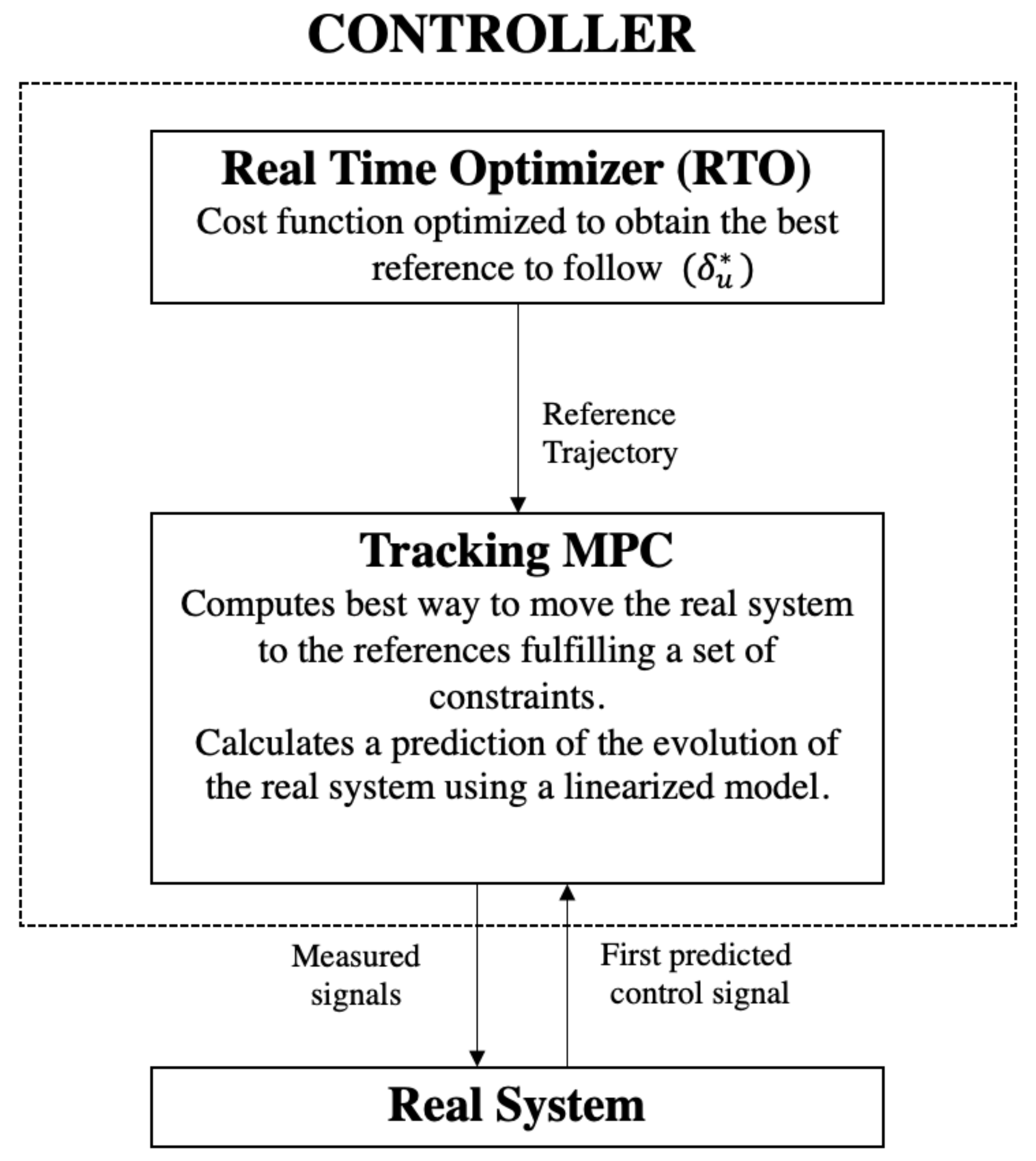
  • A controller design, tested in a case study, reducing both irrigation and electricity costs at farm scale without compromising crop yield.
    The controller is composed of two layers. The first one is real-time optimization (RTO) with a nonlinear model, and its function is to compute the best economic trajectory, taking into account the periodic behavior of the main system variables, the constraints related to the soil moisture, and the water and electricity costs. The second layer is based on the MPC for tracking developed in [24], which guarantees convergence and recursive feasibility even when the parameters of the cost function change with time. It adaptation makes it possible to take into account the uniformity of irrigation, as analyzed in [25], avoiding decreasing crop yield.
  • Comparison between the proposed controller (RTO + MPC) strategy and a classical irrigation strategy, taking into account the water and energy costs.
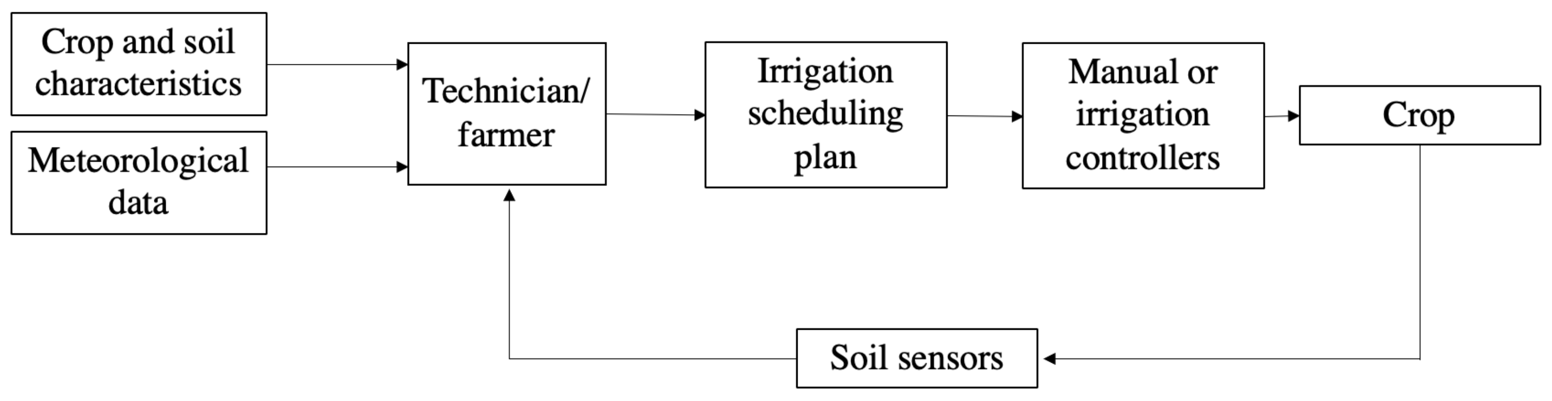
The paper is structured as follows: Section 2 presents the system structure. Section 3 introduces the nonlinear dynamical model that characterizes the dynamics of soil water, taking into account the relationship between soil moisture and transpiration to determine the crop yield. Section 4 formulates the proposed controller (RTO + MPC) and its associated variables, constraints and objectives. Section 5 presents the simulation results over a real case study of strawberries in the province of Huelva (Spain). Finally, Section 6 draws the main conclusions of this paper.

2. System Structure

The main goal for optimizing irrigation is saving water, fertilizer and energy, minimizing costs without decreasing yield. Traditionally, irrigation decisions are made by farmers or field technicians.
Figure 1 shows the scheme of the traditional irrigation strategy considering the use of soil sensors. The technician/farmer analyzes the information, such as crop and soil characteristics, the meteorological data and the soil sensor data, collected from the crop field to formulate an irrigation scheduling plan. This irrigation scheduling plan is executed manually or through irrigation controllers.
Based on this concept, our proposed controller considers the water soil dynamics using an agro-hydrological model with constraints on the upper and bottom soil moisture levels. Once a day (every 24 h), the RTO obtains the soil moisture value from the sensor, adjusting the optimal signal to the energy costs, and changes the reference (best irrigation schedule), which will be sent to the MPC so that it can follow it. The MPC obtains the sensor data every 15 min and creates a trajectory, seeking to reach the RTO signal, saving water and energy without compromising the crop yield. Figure 2 shows the proposed controller scheme.

3. Model Description

The most common way to measure the soil moisture in cultivated plots is through the volumetric water content (VWC), which is the ratio of water volume to soil volume. This variable plays a crucial role in irrigation control. Available water (AW) is the range between the permanent wilting point (PWP), the soil moisture level at which plants cannot extract water from the soil, and below the field capacity (FC), the amount of water content held in soil after excess water has drained away. Moreover, there is a soil moisture range where the plant can grow without compromising the crop yield, named readily available water (RAW). Management allowed depletion (MAD) is the desired soil–water deficit at the time of irrigation [26]. The MAD used in the proposed model is the lower limit of RAW. Providing irrigation water at this limit, the crop does not suffer from water stress, which can reduce yields.
A crucial and yet overlooked aspect in the design of advanced controllers for irrigation systems is to consider an appropriate dynamical model to predict the soil water fluxes. Expert agronomists rely on information from several sources (soil, plant, and atmosphere), to properly manage the irrigation requirements of the crops [27].

3.1. Soil Water Dynamics

Here, we rely on an extended version of the model in [28], which consists of nonlinear partial differential equations, characterizing the hydrological cycle between the crop, the soil, and the atmosphere, further developed and tested by the authors of this paper in [29]. With this hydrological model, a predictive controller (RTO + MPC) can optimize irrigation using the soil as a water buffer, where the variations are caused by both inflows, irrigation, and precipitation and outflows, transpiration, and evaporation. We assume that the irrigation water enters the ground in the same way as precipitation, and only vertical hydrological dynamics are considered. The soil is divided into N + 1 layers: the surface layer, root zone (further divided into N 1 layers), and drainage zone are shown in Figure 3. The equations to describe the water dynamics are as follows:
d θ 1 d t = 1 D 1 I r r + P t Q 1 , i ( θ 1 , θ 2 ) 1 ρ w E
d θ i d t = 1 D i Q ^ i ( θ i , θ i + 1 ) 1 ρ w T 3 , i = 2 N 1
d θ N d t = 1 D N + 1 Q N , N + 1 ( θ N , θ N + 1 ) Q N + 1 ( θ N + 1 )
where θ i is the volumetric water content of each layer (soil moisture), Q i , i + 1 are the water flux between layers with the nonlinear dependence of θ i described in [28], Q ^ i = Q i 1 , i Q i , i + 1 , D i is the soil thickness of each layer, I r r is the irrigation depth, P t is the precipitation, Q N + 1 is the flux out of the drainage zone, E and T are evaporation from the soil surface and transpiration from the vegetation canopy, respectively, and ρ w is the water density. The soil moisture at different levels is thus computed at each time step as influenced by precipitation, evaporation, transpiration, and drainage. The flux of the drainage zone is free by default [30] and this flux is important to know because drainage is water lost as a consequence of over-irrigation.
To characterize the water flows between zones, Equation (36) in [31] can be used, which, after a finite difference discretization, yields:
Q i , i + 1 = ψ ^ 0.5 D ^ + 1 K ^ ψ ^
ψ ^ = ψ i + 1 ψ i
D ^ = D i + D i + 1
K ^ = K i ψ i K i + 1 ψ i + 1
ψ i , i + 1 = ψ s a t θ i θ s a t b
K i = K s a t θ i θ s a t 2 b + 3
where K i is the hydraulic conductivity of each layer, ψ i is the matrix potential of each layer, θ s a t is the soil porosity, K s a t is the hydraulic conductivity at saturation, b is an empirical parameter related to soil texture, and the drainage out of the bottom layer is assumed to be K N + 1 . The runoff occurs when surface soil water content θ 1 exceeds the porosity θ s a t .

3.2. Crop Yield

Transpiration is the process of water movement through a plant and its evaporation from aerial parts, such as leaves, stems, and flowers. Water is absorbed by roots from the soil, and of all the water absorbed by plants, less than 5% remains in the plant for growth [32]; the crop consumes the most water in the process of transpiration.
According to [33], the water availability in the soil can often limit transpiration, reducing crop yields. The most common method to determine the water content in the soil is through soil moisture sensors.
For strawberry, the case study in this paper, the equation relating the soil moisture to transpiration was extracted from [34]:
T a = 5 × 10 6 x p 3 0.0015 x p 2 + 0.1564 x p 2.817
where T a is the actual crop transpiration and x p is the soil water content as a percentage.
Considering the relationship between soil moisture and transpiration, crop yield can be estimated, because, according to [35], only the transpiration portion directly influences the crop yield. The crop water production function presented in [36] is:
( 1 Y a Y m ) = K y ( 1 T a T m )
K y = 1.01 ± S E 0.0083
where Y a is actual crop yield, Y m is the potential crop yield, T a is the actual transpiration, and T m is the potential transpiration. The potential crop yield is between 0 and 1, T m is governed by atmospheric conditions and crop characteristics [37], and K y is the slope of the linear relationship.
Water yield production functions are useful for irrigation scheduling, for the estimation of water requirements and maximum yield, and for the determination of irrigation application efficiency [38].

4. Model Predictive Control Algorithm

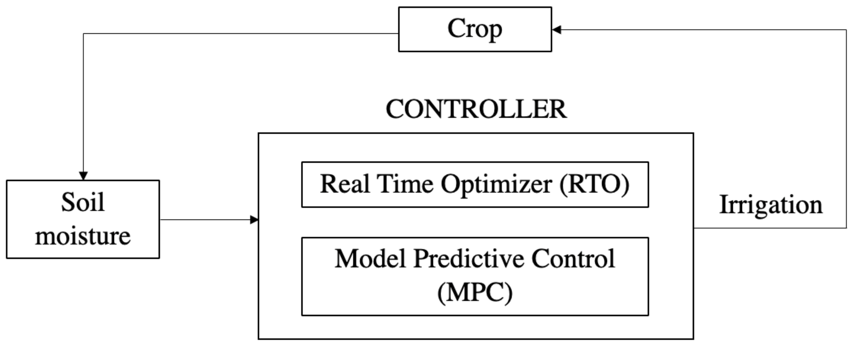
4.1. Predictive Control Hierarchical Structure

Based on Figure 2, the structure of the proposed economic and periodic predictive controller is shown in Figure 4. The input for the tracking MPC is an optimized reference trajectory, which is obtained from a real-time optimizer layer (RTO). Once daily, this RTO obtains the soil moisture sensor value and considers a complex economic function, providing the best periodic trajectory, which must be tracked to obtain the best results in controlling a linear or nonlinear model.
The tracking MPC layer makes use of a linearized version of the model Equations (1a), (1b) and (1c) to predict, during a time window equal to the system period (1 day), the evolution of the soil moisture, the water, and energy consumption. This layer must move the system to maintain the soil moisture as close as possible to the value given by the RTO. This periodic aspect helps to ensure the controller’s stability since the system does not have to stabilize in an operating point but a periodic trajectory. However, following a classic receding horizon paradigm, only the first control action is applied and, after that, the system outputs (soil moisture) are measured again with the sensor and the MPC tracking problem is recursively solved. It is important to remark that the tracking layer tries to approach the optimal references. This second layer guarantees the recursive feasibility and stability even when changes in certain parameters of the reference ( δ u ) occur; this layer follows the developments in [24]. This is an interesting controller that increases the reachability region compared to other classic tracking controllers.
The control objective in the second layer is usually to derive a control law δ u ( k ) = κ ( x ( k ) , w ( k ) ) such that the evolution of the closed-loop system fulfils the constraints (usually, the maximum and minimum in the soil moisture and irrigation flow) and the periodic tracking converge asymptotically to the nearest signal to that computed by the RTO ( δ u ).

4.2. Model Linearization

The nonlinear agro-hydrological model Equations (1a), (1b) and (1c) are too complex for MPC. To simplify the MPC work, a linear approximation is found to the nonlinear model at equilibrium points, where the crop has a maximum yield. A linear time-invariant (LTI) model is obtained from the linearization:
x ( k + 1 ) = A x ( k ) + B u ( k ) + B d w ( k )
y ( k ) = C x ( k )
Model Equations (5a) and (5b) have four constant matrices, where A is the system matrix, B is the control matrix, B d is the disturbance matrix, and C is the output matrix. Furthermore, k is the time index, the x ( k ) R 4 represents the states of the model, y ( k ) the output system, u ( k ) R 1 represents the control action, and w ( k ) R 2 the disturbances associated with this model. In this case, the states (and outputs) of the dynamical model are the soil moisture in every layer (output), of which the last layer is dismissed because it has the same behavior as layer 4 and this layer could be used to determine the water loss; the control action is the irrigation (input) and the disturbances are transpiration T and evaporation E.
The linearization was carried out using the System Identification in MATLAB, employing an algorithm called Prediction Error Minimization (PEM) and simulated input–output data. The comparison between some of the outputs (soil moistures) of the nonlinear model Equations (1a),(1b) and (1c), and the linearized model is shown in Figure 5, where the first and second layer show good identification, and the third and fourth figure apparently show a weaker fit with the nonlinear model, but the identification range is very small (0.001 cm 3 cm 3 ) in comparison with the range between PWP and saturation soil moisture [0.09 0.395] cm 3 cm 3 .

4.3. Economic and Periodic Model Predictive Control

In our economic and periodic MPC formulation for farm irrigation systems, both the soil moisture ( x ( k ) ) and irrigation depth ( u ( k ) ) are restricted within limits related to the crop water requirements and the irrigation system, respectively. Moreover, the system performance is a weighted combination of soil moisture, water consumption, and energy and water costs. These terms are captured by a quadratic economic cost function V p ( k , x , u ) , which depends on both the system state and control inputs.
In this paper, we focus on the periodic operation of a closed-loop system with a fixed period Y of 24 h. The quasi-periodic behavior of the main dynamic variables involved at a farm scale (radiation, crop transpiration, electricity prices) enables us to take advantage of a periodic RTO and tracking layer to achieve better performance, taking into account that we are using a linear model instead of a nonlinear model.
The main goal of this control structure consists of managing the irrigation to achieve optimal economic performance, which optimizes the cost function, reducing the irrigation depth and the costs associated with the water and energy. This performance cost function V p is used by a real-time optimization (RTO) layer to provide an optimal trajectory. The optimal trajectory to operate the system is derived from the solution of the following optimization problem(6a), (6b), (6c) and (6d) where the initial state is a free variable:
min x ( 0 ) , u T k = 0 Y 1 V p ( x ( 0 ) , u T )
s . t . x ( k + 1 ) = A x ( k ) + B u ( k ) + B d w ( k ) ,
( x ( k ) , u ( k ) ) Z r , k 0 ,
x ( 0 ) = x ( Y )
where x are the states, and the set Z r is a closed polyhedron that encloses the above-mentioned restrictions that affect the soil moisture and irrigation depth. The optimal state and input trajectories (bold letters denote trajectories of signals over the prediction horizon/period) are x and u , respectively.
The optimal solution ( x T , u T ) of problem (6a) ( P P ( x , w ) ) is used by the tracking optimization problem, which is denoted as P N ( x , w ) . The objective of this problem is to move the real system to the nearest position to the optimal trajectory ( x T , u T ) .
min x 0 r , u r , u V N ( x , x , u , w ; x 0 r , u r , x r , w )
s . t . x ( 0 ) = x ( k )
x ( k + 1 ) = A x ( k ) + B u ( k ) + B d w ( k )
y ( k ) = C x ( k ) + C u ( k ) k Z N
( x , u ) Z r
x ( N ) = x r ( N )
x r ( k + 1 ) = A x r ( k ) + B u r ( k ) + B d w ( k )
( x r , u r ) Z r
y r ( k ) = C x r ( k ) + C u r ( k ) k Z T
x r ( 0 ) = x r ( Y ) i = 1 Y
where x r and u r are reachable trajectories by the linear model of the controller used to avoid a problematic situation (loss of recursive feasibility, etc.) for the MPC controller. For more details, see [39].
The cost function of this controller, considering the respective matrices’ weights ( Q , R , W , S ) , is defined as follows:
V N ( x , w ; x 0 r , u r , u ) = V S ( x , w ; x 0 r , x r , x , u r , u ) + V T ( x 0 r , u r )
and
V S = k = 0 N 1 x ( k ) x r ( k ) Q 2
+ u ( k ) u r ( k ) R 2 V T ( x 0 r , u r ) = k = 0 Y 1 x r ( k ) x T ( k ) W 2
+ u r ( k ) u T ( k ) S 2
In general, the initial soil moisture is an argument for the tracking optimization problem, and considering that this controller presents a large reachability region and the size of the admissibility for the soil moisture, the possibility of the optimization problem becoming unfeasible is strongly reduced.
The constraints of the optimization variables are divided into four groups: constraint (7a) imposes that the initial state of the predicted trajectory is equal to the state of the system at time step k; constraints (7b) and (7c) provide the predicted state and input trajectories; constraint (7f) states that the predicted state must reach the artificial reference in Y steps; and constraints (7g)–(7i) provide the artificial reference state and input trajectories. The artificial inputs and states are the decision variables of the optimization problem. These trajectories are reachable trajectories by the model and must be near to the reference, or if possible, must converge to the reference if the reference provided by the RTO is reachable by the model.
It must be noted that we propose the use of a nominal controller, not a robust controller. We avoid unfeasibilities by using a soft constraint in the lower constraints of the soil moisture.

4.4. Economic Cost Function for Agriculture

The economic cost function is composed of four main terms. The first term weighs deviations of the soil moisture below the setpoint established as the minimum soil water content permissible (MAD). The second term uses a time-varying weight to minimize the energy cost related to irrigation water. The third term minimizes the use of water. Finally, the last term tries to maintain the minimum level of soil moisture that guarantees the potential (maximum) crop evapotranspiration.
V p ( x , u ) = w p 1 f 1 ( x o p ; x ) + w p 2 f 2 ( u ) + w p 3 f 3 ( u ) + w p 4 f 4 ( x )
f 1 ( x ) = k = 0 Y 1 x ( k ) x o p Q
f 2 ( u ) = k = 0 Y 1 C e l e c ( k ) u ( k )
f 3 ( u ) = k = 0 Y 1 C w a t e r u ( k )
f 4 ( x ) = k = 0 Y 1 T a ( k )
where C e n e r g y is a time-varying electric cost, C w a t e r is a fixed cost associated with the water per m 3 , x o p are the operational point values per layer established as the minimum soil water content permissible (MAD), and w p i are the corresponding weights.

5. Simulation Results

5.1. Case Study

We use a case study corresponding to a strawberry farm located in Almonte (Spain); the strawberry cultivar is Sabrina. The cultivars differ in yield and water consumption, determining different crop yields [40]. The farm soil is sandy and strawberry is cultivated under a plastic tunnel with an average size of 6.6 × 50 m. The strawberries were planted in trapezoidal raised beds measuring 0.60 m at the base, 0.50 m at the top, with a height of 0.50 m. Beds were separated by 1.1 m, so each tunnel had six beds and was covered with black plastic mulch. Two rows of plants were placed along the bed with subsurface drip irrigation tape in the center. Plants were spaced 0.25 m apart. A significant number of farmers apply water in pulses of 30–40 min [25,41]. The crops need more water at the end of the season, in June. During June, farmers apply water between 60 and 90 min a day. In this specific case, we consider the classical irrigation in pulses of 35 min twice a day: this is a total of 70 min. Water was supplied by drip irrigation using emitters spaced every 0.2 m, with a flow rate of 5 l h m at a pressure of 1 MPa. The irrigation depth was ≈6.88 l m 2 .
The classical irrigation described above and the controller irrigation system proposed in this paper are compared in terms of the quantity of water for irrigating crops, energy costs, and crop yield. The water price used in the case study is constant and equal to 0.35 Euros m 3 [42] and the electricity tariff per hour in Spain, presented in Table 1, was extracted from [43].
In all the simulation analyses, for both strategies, we use the nonlinear Equations (1a) and (1b) with the first four soil layers (except drainage layer), and the thickness of the layers (3, 12, 12, 12, centimeters) was considered. The term P t is assumed zero because the strawberries were cultivated under plastic (tunnel greenhouse).
Furthermore, note that the evapotranspiration E T c includes evaporation and transpiration. E T c is an important concept and is a common concern in hydrology, ecology, and meteorology [44]. According to [45], the transpiration T is the result of reference evapotranspiration ( E T o ), which is multiplied by the crop coefficient K c . The crop coefficient K c for the Sabrina cultivar is above 0.85 in June [46]. As the beds were covered by black plastic sheets inside polytunnels, it was assumed that the crop evapotranspiration E T c was only due to plant transpiration, because there was no evaporation from the soil [47], so E is neglected for this application. Moreover, the simulations use real values for strawberries Y corresponding to a cloudless day in June. These values are shown in Figure 6d with Y for 3 days (4320 min).
According to Equation (3), the soil moisture can be expressed as soil water content as a percentage. Undertaking a transformation to cm 3 cm 3 , the following values for a sandy soil were assumed. Field capacity (FC) value was 0.16 cm 3 cm 3 , and the permanent wilting point (PWP) was 0.09 cm 3 cm 3 . The soil characterization values [48] are shown in Table 2.
The crop yield analysis is crucial because water can be conserved by working within the RAW soil moisture range. Thus, the setpoint x o p in Equations (10a) and (10b) established as the minimum soil water content permissible was assigned to 0.15. The authors established this as the MAD value, which is around 85% of available water (FC-PWP) in the case of strawberries cultivated in Huelva. In this range of readily available water (RAW), plants are neither waterlogged nor water-stressed [26].
For this analysis, we considered homogeneous soil and crops, and irrigation uniformity influenced by filling/emptying water dynamics.

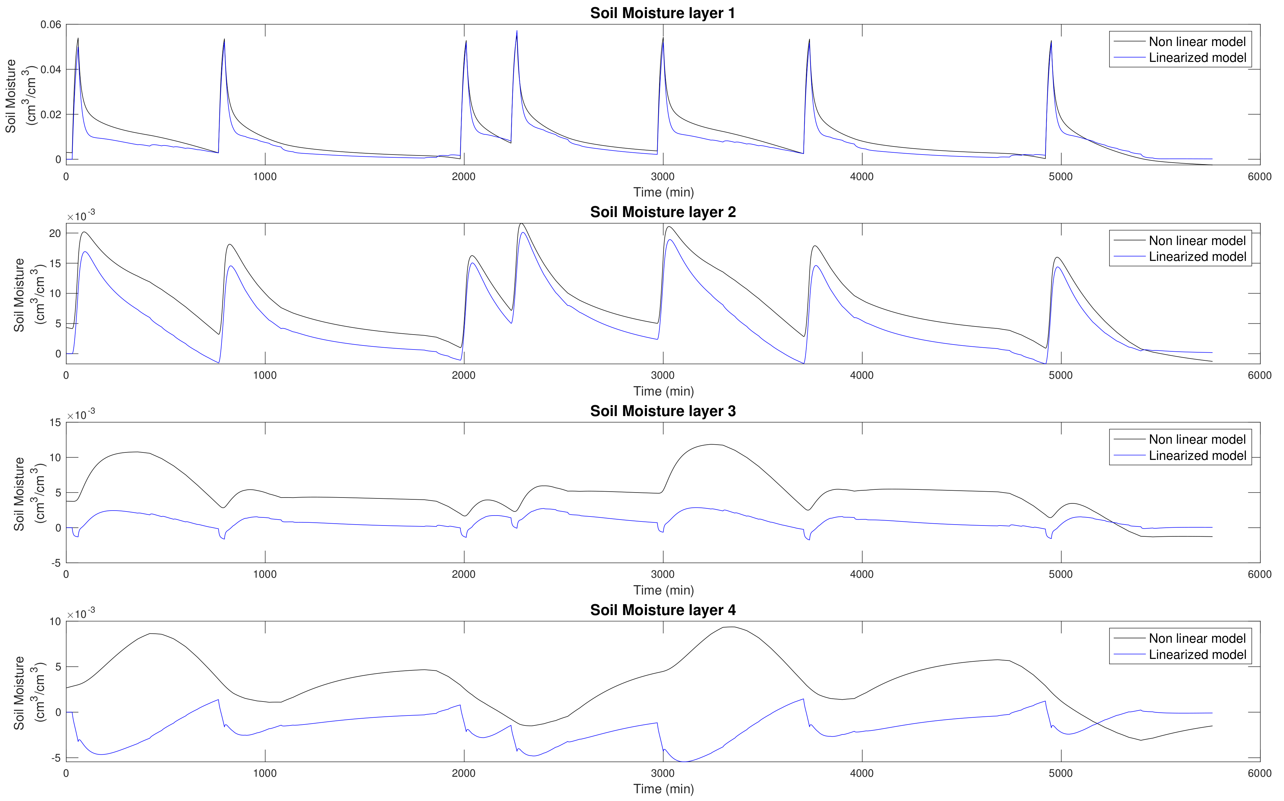
5.2. Linear Model Used in the Controller Strategy

The field capacity plays a key role when using the soil as a water buffer or reservoir because, above it, the water excess is rapidly drained. A thorough simulation analysis of the nonlinear model Equations (1a), (1b) and (1c) make it possible to estimate the field capacity. To this end, simulations with wet layers free of crops were conducted, and the points at which free drainage becomes negligible were determined. These values (soil moisture x e q , irrigation u e q , transpiration T and evaporation E) were used as equilibrium points for the model linearization.
According to the LTI model Equations (5a) and (5b), the values for equilibrium points were the following:
x e q = 0.154 0.153 0.152 0.151 cm 3 cm 3
u e q = 0
T = 0
E = 0
The model linearization around the FC with a sampling time of 15 min results in the following normalized system matrices presented in model Equations (5a) and (5b):
A = 0.1000 0.0050 0.0051 0.0146 0.4248 0.0145 0.0128 0.3353 0.2559 0.0141 0.0133 0.1218 0.008 6.9467 × 10 4 9.6372 × 10 4 0.0021
B = 0.0216 4.4488 × 10 3 1.9269 × 10 6 0.2392 2.9900 × 10 5 7.4813 × 10 7 0.1481 1.5443 × 10 5 2.5278 × 10 7 0.0035 3.9564 × 10 3 1.305 × 10 8
C = 0.3195 0.0213 0.0261 0.0426 0.0131 0.0012 0.0029 0.0955 0.0014 8.5556 × 10 4 6.2345 × 10 4 0.0427 0.0134 0.0017 0.0042 0.0165
The MPC has restrictions very near to the operational point x o p to check the controller performance. In this case study, x o p = x e q .
The constraints and weights used in RTO and MPC are summarized in Table 3. The constraints are the lowest and highest value of the soil moisture ( x m i n , x m a x ) and irrigation flow ( u m i n , u m a x ) in which the controller can work. The weights ( w p 1 , w p 2 , w p 4 ) indicate the importance of each of the cost functions for agriculture presented in Section 4.4.
In the controller, specifically in the RTO function cost, we take into account the electricity and water cost, the transpiration, and the deviation of the actual soil moisture concerning the setpoint. The weight w p 1 penalizes the soil moisture deviation from the setpoint. w p 2 , w p 3 gives greater importance to the minimization of electricity and water costs and w p 4 gives importance to the transpiration. The w p 1 is very small because the priority is to minimize the irrigation, taking into account the electricity cost, water cost, and transpiration. The RTO gives a reference signal to the MPC and tries to track this signal, taking into account the soil moisture operational point.
As detailed in Section 4, the proposed controller is composed of RTO + MPC. The RTO uses the linearized model to obtain the best signal that the MPC can follow. In Figure 6a, we present the RTO and proposed controller (RTO + MPC) signal: the proposed controller uses the linearized model for evaluation. With this, we can confirm that the controller perfectly follows the RTO signal and irrigation begins when the electricity prices are lower.
Both irrigation strategies, the classical and the proposed (RTO + MPC) controller strategy, were also evaluated using the real agro-hydrological model Equations (1a), (1b) and (1c). In Figure 6b, the results are slightly different because the real agro-hydrological model is highly nonlinear. It similarly achieves periodicity, important for irrigation systems.

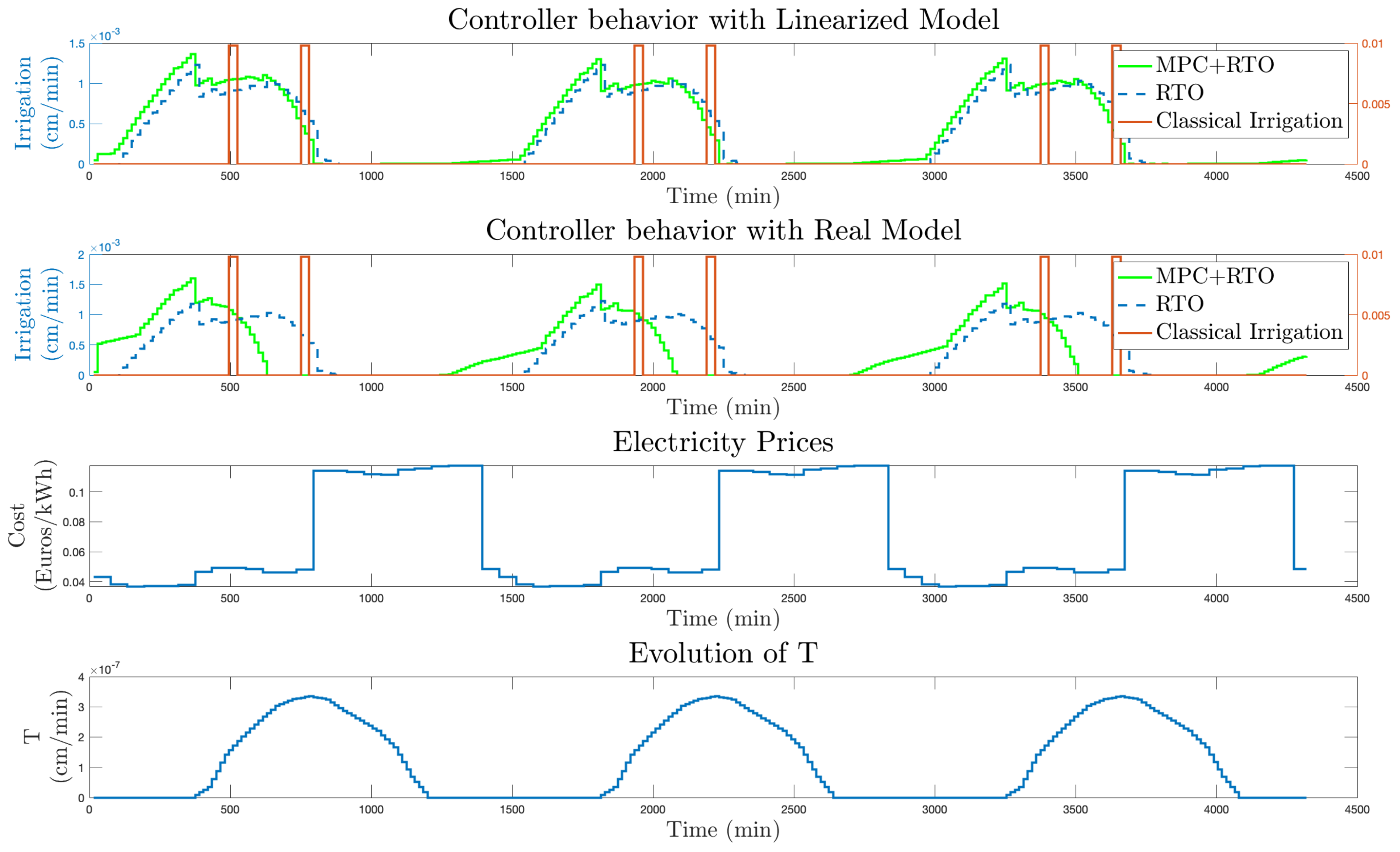
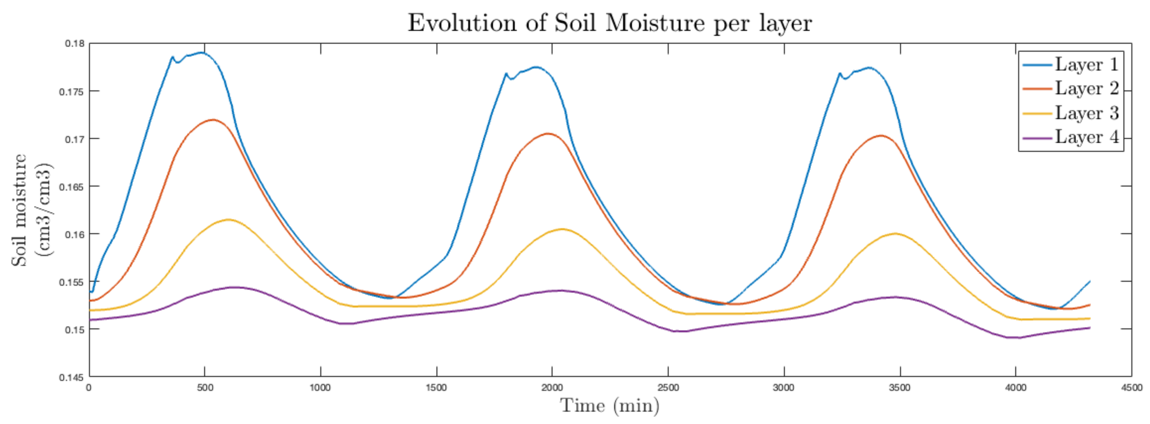
5.3. Results Using the Real (Nonlinear) Agro-Hydrological Model to Simulate Soil Moisture Evolution

We compare two irrigation strategies, classical irrigation and the proposed RTO + MPC irrigation strategy. Both scenarios take into account the evolution of the electricity price and transpiration, as depicted in Figure 6c,d.
Both strategies were evaluated using simulations with a duration of 3 days (4320 min) during the month of June, and in order to simplify the simulation, we assumed that the energy consumption was 0.4 kWh m 3 . Figure 6b shows the amount of applied water for the classical irrigation and proposed controller strategy (RTO + MPC) together with the references provided by RTO. The proposed controller tries to trigger irrigation when electricity prices are lower—see Figure 6c—without compromising crop yield—see Figure 6a,b.
The soil moisture evolution per layer in the described classical irrigation and proposed controller (RTO + MPC) strategy is shown in Figure 7 and Figure 8, respectively. The classical irrigation strategy’s operational range is within [0.145 0.208] cm 3 cm 3 and the proposed (RTO + MPC) controller’s operational range is within [0.149 0.179] cm 3 cm 3 . Therefore, soil moisture layers are above the operational point at almost any time cm 3 cm 3 .
The soil moisture signal is given by the controller strategy (MPC + RTO) to track the signal given by the RTO and stay above the MAD in the four layers (Figure 9). Soil moisture in layers 1 and 2 was above FC at a certain time, which is normal, since the soil water flows from the first layers and seeps down into the lower soil layers. This downward movement fulfils deeper layers. However, even in the last layer (layer 4), the soil moisture does not drop below the MAD level (0.15 cm 3 cm 3 ). Therefore, within these soil moisture ranges and considering the Equations (3), (4a) and (4b), the crop yield was maximum for both the classical and proposed controller (RTO + MPC) strategies.
Furthermore, a simulation of 30 days during the whole month of June was also conducted, with the same conditions as the 3-day simulation and taking advantage of the periodicity of the controller. A summary of the obtained results over 30 days is presented in Table 4.
Crop water requirements during the whole month were around 157.5 l m 2 . Therefore, the total water applied to the crop was higher than 157.5 l m 2 so as not to reduce the crop yield in both irrigation strategies (Table 4). For the classical and proposed (RTO + MPC) irrigation strategies, irrigation application efficiency was 76.2% and 94.3%, respectively. Thus, the proposed controller (RTO + MPC) strategy was more efficient than the classical irrigation strategy. Likewise, the proposed controller (RTO + MPC) strategy reduced the energy cost by more than 50% in comparison to the classical irrigation strategy, without compromising the crop yield.
Based on the results obtained in these simulations, it can be considered that the predictive control proposed in this work (RTO+ MPC) is an efficient tool for optimal irrigation management. The use of this type of predictive controller in irrigation scheduling broadens the possibilities of optimizing irrigation, considering multiple management variables in real time. In this sense, we encourage the research and technical community to use this type of predictive controller in future scenarios of multiple IoT devices for monitoring the different variables in the soil–plant–atmosphere–irrigation system.

6. Conclusions

A predictive controller has been developed for optimal irrigation management at a farm scale. The proposed controller strategy incorporates a multi-layer agro-hydrological model and an economic cost function. The economic cost function is composed of four terms, deviation of the soil moisture from an operational point, minimization of energy costs, minimization of water costs, and the last term to maintain the potential crop evapotranspiration to guarantee the maximum yield.
The proposed predictive controller (RTO + MPC) was compared with a classical irrigation strategy in a real scenario, showing a significant reduction in water consumption and energy costs without compromising crop production.
Because of the results obtained in this work, the authors wish to emphasize that in order to implement an irrigation control system based on soil moisture, it is important to consider the real (nonlinear) water dynamics in the soil to ensure that the results are representative of reality.
This work has been an initial step towards implementing automatic irrigation based on multivariable inputs obtained from IoT-based devices. The presented predictive controller has high potential to improve not only water use efficiency but also energy costs, without reducing crop yields. Further studies will reveal further details of their benefits for the economic optimization of irrigation scheduling.

Author Contributions

Conceptualization, G.C., D.L. and P.M.; methodology, P.M., M.P. and G.C.; software, G.C. and M.P.; validation, M.P. and G.C.; formal analysis, G.C. and D.L.; investigation, G.C.; writing—original draft preparation, G.C., M.P., P.M., D.L.; writing—review and editing, G.C., D.L. and M.P.; visualization, G.C. and D.L.; supervision, M.P. and P.M.; project administration, P.M.; funding acquisition, P.M. All authors have read and agreed to the published version of the manuscript.

Funding

This work has been partially funded by the project “INNOREGA: RIEGO SOSTENIBLE BASADO EN MONITORIZACIÓN DISTRIBUIDA E INTELIGENCIA ARTIFICIAL (PP.AVA. AVA2019.024), funded by FEDER 2014–2020 (“Programa Operativo de Crecimiento Inteligente”, Junta de Andalucía). The authors would like to acknowledge Junta de Andalucía and the European Regional Development Fund for partially funding this work under the project IRRIGATE (Grant PY20 RE 017).

Institutional Review Board Statement

Not applicable.

Informed Consent Statement

Not applicable.

Data Availability Statement

Not applicable.

Acknowledgments

The authors wish to acknowledge the contribution of Pedro Gavilán as leader of the INNOREGA project (PP.AVA.AVA2019.024).

Conflicts of Interest

The authors declare no conflict of interest.

References

  1. Enescu, F.M.; Bizon, N.; Onu, A.; Răboacă, M.S.; Thounthong, P.; Mazare, A.G.; Șerban, G. Implementing blockchain technology in irrigation systems that integrate photovoltaic energy generation systems. Sustainability 2020, 12, 1540. [Google Scholar] [CrossRef] [Green Version]
  2. García, I.F.; Montesinos, P.; Poyato, E.C.; Díaz, J.R. Optimal design of pressurized irrigation networks to minimize the operational cost under different management scenarios. Water Resour. Manag. 2017, 31, 1995–2010. [Google Scholar] [CrossRef]
  3. European Commission. Farm to Fork Strategy; European Commission: Brussels, Belgium, 2019. [Google Scholar]
  4. European Commission. Communication from the Commission to the European Parliament, the European Council, the Council, the European Economic and Social Committee and the Committee of the Regions; The European Green Deal. COM/2019/640 Final; European Commission: Brussels, Belgium, 2019. [Google Scholar]
  5. Incrocci, L.; Thompson, R.B.; Fernandez-Fernandez, M.D.; De Pascale, S.; Pardossi, A.; Stanghellini, C.; Rouphael, Y.; Gallardo, M. Irrigation management of European greenhouse vegetable crops. Agric. Water Manag. 2020, 242, 106393. [Google Scholar] [CrossRef]
  6. Domínguez-Niño, J.M.; Oliver-Manera, J.; Girona, J.; Casadesús, J. Differential irrigation scheduling by an automated algorithm of water balance tuned by capacitance-type soil moisture sensors. Agric. Water Manag. 2020, 228, 105880. [Google Scholar] [CrossRef]
  7. McCarthy, A.C.; Hancock, N.H.; Raine, S.R. Advanced process control of irrigation: The current state and an analysis to aid future development. Irrig. Sci. 2013, 31, 183–192. [Google Scholar] [CrossRef]
  8. Casadesús, J.; Mata, M.; Marsal, J.; Girona, J. A general algorithm for automated scheduling of drip irrigation in tree crops. Comput. Electron. Agric. 2012, 83, 11–20. [Google Scholar] [CrossRef]
  9. Doorenbos, J. Guidelines for predicting crop water requirements. FAO Irrig. Drain. Pap. 1977, 24, 1–179. [Google Scholar]
  10. Muñoz-Carpena, R.; Dukes, M.D. Automatic Irrigation Based on Soil Moisture for Vegetable Crops; University of Florida: Gainesville, FL, USA, 2005. [Google Scholar]
  11. Cáceres, R.; Casadesús, J.; Marfà, O. Adaptation of an automatic irrigation-control tray system for outdoor nurseries. Biosyst. Eng. 2007, 96, 419–425. [Google Scholar] [CrossRef]
  12. Perea, R.G.; Poyato, E.C.; Díaz, J.R. Forecasting of applied irrigation depths at farm level for energy tariff periods using Coactive neuro-genetic fuzzy system. Agric. Water Manag. 2021, 256, 107068. [Google Scholar] [CrossRef]
  13. Rodríguez Díaz, J.; Camacho Poyato, E.; Blanco Pérez, M. Evaluation of water and energy use in pressurized irrigation networks in Southern Spain. J. Irrig. Drain. Eng. 2011, 137, 644–650. [Google Scholar] [CrossRef]
  14. García, I.F.; Díaz, J.R.; Poyato, E.C.; Montesinos, P.; Berbel, J. Effects of modernization and medium term perspectives on water and energy use in irrigation districts. Agric. Syst. 2014, 131, 56–63. [Google Scholar] [CrossRef]
  15. Lozano, D.; Arranja, C.; Rijo, M.; Mateos, L. Simulation of automatic control of an irrigation canal. Agric. Water Manag. 2010, 97, 91–100. [Google Scholar] [CrossRef] [Green Version]
  16. Romero, R.; Muriel, J.; García, I.; de la Peña, D.M. Research on automatic irrigation control: State of the art and recent results. Agric. Water Manag. 2012, 114, 59–66. [Google Scholar] [CrossRef]
  17. Van Overloop, P.; Clemmens, A.; Strand, R.; Wagemaker, R.; Bautista, E. Real-time implementation of model predictive control on Maricopa-Stanfield irrigation and drainage district’s WM canal. J. Irrig. Drain. Eng. 2010, 136, 747–756. [Google Scholar] [CrossRef]
  18. Delgoda, D.; Malano, H.; Saleem, S.K.; Halgamuge, M.N. Irrigation control based on model predictive control (MPC): Formulation of theory and validation using weather forecast data and AQUACROP model. Environ. Model. Softw. 2016, 78, 40–53. [Google Scholar] [CrossRef]
  19. Shang, C.; Chen, W.H.; Stroock, A.D.; You, F. Robust model predictive control of irrigation systems with active uncertainty learning and data analytics. IEEE Trans. Control Syst. Technol. 2019, 28, 1493–1504. [Google Scholar] [CrossRef] [Green Version]
  20. McCarthy, A.C.; Hancock, N.H.; Raine, S.R. Simulation of irrigation control strategies for cotton using Model Predictive Control within the VARIwise simulation framework. Comput. Electron. Agric. 2014, 101, 135–147. [Google Scholar] [CrossRef] [Green Version]
  21. Mao, Y.; Liu, S.; Nahar, J.; Liu, J.; Ding, F. Soil moisture regulation of agro-hydrological systems using zone model predictive control. Comput. Electron. Agric. 2018, 154, 239–247. [Google Scholar] [CrossRef]
  22. Moreno, M.A.; Carrión, P.A.; Planells, P.; Ortega, J.F.; Tarjuelo, J.M. Measurement and improvement of the energy efficiency at pumping stations. Biosyst. Eng. 2007, 98, 479–486. [Google Scholar] [CrossRef]
  23. Jiménez-Bello, M.; Alzamora, F.M.; Soler, V.B.; Ayala, H.B. Methodology for grouping intakes of pressurised irrigation networks into sectors to minimise energy consumption. Biosyst. Eng. 2010, 105, 429–438. [Google Scholar] [CrossRef]
  24. Limon, D.; Pereira, M.; Muñoz de la Peña, D.; Alamo, T.; Jones, C.N.; Zeilinger, M.N. MPC for Tracking Periodic References. IEEE Trans. Autom. Control 2016, 61, 1123–1128. [Google Scholar] [CrossRef] [Green Version]
  25. Lozano, D.; Ruiz, N.; Baeza, R.; Contreras, J.I.; Gavilán, P. Effect of pulse drip irrigation duration on water distribution uniformity. Water 2020, 12, 2276. [Google Scholar] [CrossRef]
  26. Allen, R.G.; Pereira, L.S.; Raes, D.; Smith, M. Crop Evapotranspiration-Guidelines for Computing Crop Water Requirements-FAO Irrigation and Drainage Paper 56; FAO: Rome, Italy, 1998; Volume 300, p. D05109. [Google Scholar]
  27. Puerto, P.; Domingo, R.; Torres, R.; Pérez-Pastor, A.; García-Riquelme, M. Remote management of deficit irrigation in almond trees based on maximum daily trunk shrinkage. Water relations and yield. Agric. Water Manag. 2013, 126, 33–45. [Google Scholar] [CrossRef]
  28. Qin, J.; Liang, S.; Yang, K.; Kaihotsu, I.; Liu, R.; Koike, T. Simultaneous estimation of both soil moisture and model parameters using particle filtering method through the assimilation of microwave signal. J. Geophys. Res. Atmos. 2009, 114. [Google Scholar] [CrossRef]
  29. Cáceres Rodríguez, G.; Millán Gata, P.; Pereira Martín, M.; Lozano, D. Economic model predictive control for smart and sustainable agriculture. In Proceedings of the European Control Conferences ECC, Saint-Petersburg, Russia, 12–15 May 2020. [Google Scholar]
  30. Raoult, N.; Delorme, B.; Ottlé, C.; Peylin, P.; Bastrikov, V.; Maugis, P.; Polcher, J. Confronting Soil Moisture Dynamics from the ORCHIDEE Land Surface Model with the ESA-CCI Product: Perspectives for Data Assimilation. Remote Sens. 2018, 10, 1786. [Google Scholar] [CrossRef] [Green Version]
  31. Sellers, P.; Randall, D.; Collatz, G.; Berry, J.; Field, C.; Dazlich, D.; Zhang, C.; Collelo, G.; Bounoua, L. A revised land surface parameterization (SiB2) for atmospheric GCMs. Part I: Model formulation. J. Clim. 1996, 9, 676–705. [Google Scholar] [CrossRef]
  32. Sterling, T.M. Transpiration: Water movement through plants. J. Nat. Resour. Life Sci. Educ. 2005, 34, 123. [Google Scholar] [CrossRef]
  33. Tanner, C.; Sinclair, T. Efficient water use in crop production: Research or research? In Limitations to Efficient Water Use in Crop Production; American Society of Agronomy: Madison, WI, USA, 1983; pp. 1–27. [Google Scholar]
  34. Martínez-Ferri, E.; Carrera, M.; Soria, C.; Ariza, M.T. Cultivar choice as a water saving strategy in strawberry. Book of Abstracts BP2021, Proceedings of the Reunión de la Sociedad de Biología de Plantas/XVII Congreso Hispano-luso de Biología de Plantas, Vigo, Spain, 7–8 July 2021. pp. 442–443. Available online: https://bp2021.eu/wp-content/uploads/2021/08/book_of_abstracts_bp2021.pdf (accessed on 1 September 2021).
  35. De Wit, C. Transpiration and Crop Yields: Agricultural Research Reports 64.6; PUDOC: Wageningen, The Netherlands, 1958. [Google Scholar]
  36. Serrano, L.; Carbonell, X.; Save, R.; Marfà, O.; Peñuelas, J. Effects of irrigation regimes on the yield and water use of strawberry. Irrig. Sci. 1992, 13, 45–48. [Google Scholar] [CrossRef]
  37. Kroes, J.; Van Dam, J.; Bartholomeus, R.; Groenendijk, P.; Heinen, M.; Hendriks, R.; Mulder, H.; Supit, I.; Van Walsum, P. SWAP Version 4; Technical Report; Wageningen Environmental Research: Wageningen, The Netherlands, 2017. [Google Scholar]
  38. Stewart, J.; Hagan, R.; Pruitt, W.; Kanks, R.; Riley, J.; Danilson, R.; Franklin, W.; Jackson, E. Optimizing Crop Production through Control of Water and Salinity Levels; Utah Water Research Laboratory: Logan, UT, USA, 1977; pp. 1–151. [Google Scholar]
  39. Limon, D.; Pereira, M.; De La Peña, D.M.; Alamo, T.; Grosso, J.M. Single-layer economic model predictive control for periodic operation. J. Process Control 2014, 24, 1207–1224. [Google Scholar] [CrossRef] [Green Version]
  40. Ariza, M.T.; Miranda, L.; Gómez-Mora, J.A.; Medina, J.J.; Lozano, D.; Gavilán, P.; Soria, C.; Martínez-Ferri, E. Yield and Fruit Quality of Strawberry Cultivars under Different Irrigation Regimes. Agronomy 2021, 11, 261. [Google Scholar] [CrossRef]
  41. Morillo, J.G.; Díaz, J.A.R.; Camacho, E.; Montesinos, P. Linking water footprint accounting with irrigation management in high value crops. J. Clean. Prod. 2015, 87, 594–602. [Google Scholar] [CrossRef]
  42. Chamorro, J. Sobre el Precio del Agua para la Agricultura; iAgua: Madrid, Spain, 2018. [Google Scholar]
  43. Selectra. Tarifa de luz en España; Selectra: Madrid, Spain, 2020. [Google Scholar]
  44. Zhang, S.; Wen, X.; Wang, J.; Yu, G.; Sun, X. The use of stable isotopes to partition evapotranspiration fluxes into evaporation and transpiration. Acta Ecol. Sin. 2010, 30, 201–209. [Google Scholar] [CrossRef]
  45. Lozoya, C.; Mendoza, C.; Mejía, L.; Quintana, J.; Mendoza, G.; Bustillos, M.; Arras, O.; Solís, L. Model predictive control for closed-loop irrigation. IFAC Proc. Vol. 2014, 47, 4429–4434. [Google Scholar] [CrossRef] [Green Version]
  46. Lozano, D.; Ruiz, N.; Gavilán, P. Consumptive water use and irrigation performance of strawberries. Agric. Water Manag. 2016, 169, 44–51. [Google Scholar] [CrossRef]
  47. García Morillo, J.; Rodríguez Díaz, J.; Camacho, E.; Montesinos, P. Drip irrigation scheduling using HYDRUS 2-D numerical model application for strawberry production in South-West Spain. Irrig. Drain. 2017, 66, 797–807. [Google Scholar] [CrossRef]
  48. Clapp, R.B.; Hornberger, G.M. Empirical equations for some soil hydraulic properties. Water Resour. Res. 1978, 14, 601–604. [Google Scholar] [CrossRef] [Green Version]
Figure 1. Operation diagram of the traditional irrigation strategy.
Agronomy 11 01810 g001
Figure 2. Schematic diagram of the proposed predictive controller (RTO + MPC).
Agronomy 11 01810 g002
Figure 3. A schematic of the soil layer model with the proposed division into N + 1 layers.
Agronomy 11 01810 g003
Figure 4. Flowchart of the proposed controller (RTO + MPC) and the real system.
Agronomy 11 01810 g004
Figure 5. Soil water content as a function of time for nonlinear and linearized models in the first four soil layers.
Agronomy 11 01810 g005
Figure 6. Scaled irrigation flow by the economic MPC controller, optimal consumption by RTO, and classical irrigation strategies during 3 days using (a) linearized and (b) real (nonlinear) model, (c) electricity prices, and (d) transpiration.
Agronomy 11 01810 g006
Figure 7. Soil moisture dynamics per soil layer for the classical irrigation strategy.
Agronomy 11 01810 g007
Figure 8. Soil moisture dynamics per soil layer for the predictive controller (RTO + MPC) irrigation strategy.
Agronomy 11 01810 g008
Figure 9. Soil moisture dynamics per soil layer of RTO trajectory and RTO + MPC predictive control.
Agronomy 11 01810 g009
Table 1. Electricity tariff per hour in Spain (not including fixed energy term or electricity bill taxes).
HourPrice [€/kWh]
00 h0.04271
01 h0.03788
02 h0.03653
03 h0.03682
04 h0.03666
05 h0.03735
06 h0.04621
07 h0.04904
08 h0.04904
09 h0.04815
10 h0.04592
11 h0.04598
12 h0.04784
13 h0.11382
14 h0.11368
15 h0.11306
16 h0.11148
17 h0.11107
18 h0.11448
19 h0.1154
20 h0.11681
21 h0.11744
22 h0.11744
23 h0.04818
Table 2. Soil hydraulic parameters used in the case study.
θ sat K sat ψ sat b Y m K y T m
Distributionuniformuniformuniformuniformuniformuniformuniform
Unit cm 3 / cm 3 cm/mincm-cm/min-cm/min
Value0.3951.056124.0511 2.153 × 10 4
Table 3. Table of constraints and weights for controller.
Controller
VariableRange/ValuesUnit
( x m a x , x m i n ) 0.20 0.09 cm 3 / cm 3
( u m i n , u m a x ) 0 cm/min
( w p 1 , w p 2 , w p 4 ) 0.01 40 40 20 -
E0cm/min
Table 4. Table of comparison between classical irrigation and the proposed controller in June.
Study TermsClassicalControllerUnits
Irrigation206.6166.5 l / m 2
Application efficiency76.294.3%
Energy variable cost65.2629.97 Euros / ha
Publisher’s Note: MDPI stays neutral with regard to jurisdictional claims in published maps and institutional affiliations.

