Land Degradation Vulnerability Mapping in a Newly-Reclaimed Desert Oasis in a Hyper-Arid Agro-Ecosystem Using AHP and Geospatial Techniques

Abstract

Modelling land degradation vulnerability (LDV) in the newly-reclaimed desert oases is a key factor for sustainable agricultural production. In the present work, a trial for using remote sensing data, GIS tools, and Analytic Hierarchy Process (AHP) was conducted for modeling and evaluating LDV. The model was then applied within 144,566 ha in Farafra, an inland hyper-arid Western Desert Oases in Egypt. Data collected from climate conditions, geological maps, remote sensing imageries, field observations, and laboratory analyses were conducted and subjected to AHP to develop six indices. They included geology index (GI), topographic quality index (TQI), physical soil quality index (PSQI), chemical soil quality index (CSQI), wind erosion quality index (WEQI), and vegetation quality index (VQI). Weights derived from the AHP showed that the effective drivers of LDV in the studied area were as follows: CSQI (0.30) > PSQI (0.29) > VQI (0.17) > TQI (0.12) > GI (0.07) > WEQI (0.05). The LDV map indicated that nearly 85% of the total area was prone to moderate degradation risks, 11% was prone to high risks, while less than 1% was prone to low risks. The consistency ratio (CR) for all studied parameters and indices were less than 0.1, demonstrating the high accuracy of the AHP. The results of the cross-validation demonstrated that the performance of ordinary kriging models (spherical, exponential, and Gaussian) was suitable and reliable for predicting and mapping soil properties. Integrated use of remote sensing data, GIS, and AHP would provide an effective methodology for predicting LDV in desert oases, by which proper management strategies could be adopted to achieve sustainable food security.

1. Introduction

The new atlas of desertification [1] defined dryland as regions where the aridity index (the ratio between the total annual precipitation to the annual potential evapotranspiration) is lower than 0.65, including hyper-arid, arid, semi-arid, and sub-humid regions. The dryland occupy nearly 40% of the world’s land area and supports about two billion of the human population, 90% of whom live in developing countries [2]. However, food security in the dryland, especially in developing countries, is threatened by human pressure on agricultural lands, climate change, and soil erosion [3]. In the drylands, a desert oasis is a promising area for establishing new communities and economic development [4]. It is an efficient eco-geographical landscape, which allows flourishing vegetation or human settlement owing to a stable water supply [5,6].

The Western Desert occupies nearly 68% of the total area of Egypt and includes several oases, i.e., Dakhla, Kharga, Bahariya, Siwa, and Farafra [7,8]. Farafra Oasis was included in the New Valley project in the 1960s aiming at exploiting the groundwater of the Nubian Sandstone aquifer (NSA) [9]. This oasis is characterized by the presence of a large quantity of groundwater with good quality, many of which appear on the surface of the earth in the wintertime, and thus, resulted in many farmlands on flat areas [10]. However, the desert oases are a fragile ecosystem and are affected by degradation hazards that threaten agricultural sustainability [4,11,12]. Salinization/alkalization, waterlogging and wind erosion are the most effective drivers for land degradation in irrigated desert oases [13,14,15]. Therefore, timely and early detection of land degradation vulnerability is crucial for sustainable agricultural production in these areas [3].

Land degradation vulnerability (LDV) is the susceptibility of an area to loss of productivity due to various factors responsible, including climatic dryness, poor soil, and vegetation quality [16]. The assessment of LDV is the process of identification and quantification of pressure on land resources owing to several factors influencing the land system quality [17]. Therefore, diagnosis of LDV is a complex process since it requires analyzing numerous measurements related to soil properties and soil-environmental covariates like climate, topography, and vegetation [3,18]. At present, multifactor vulnerability models have been developed to quantify the current situation of land degradation in many arid and hyper-arid regions [17,19,20]. These models used equal levels and ranking regardless the relative importance of each factor. This, in turn, makes the precise assessment of LDV too difficult as each variable has a different degree of influence, thereby, affecting the level of LDV [21]. Statistical-based methods, including principal component analysis/factor analysis (PCA/FA) have been widely used to estimate the weights of parameters or indicators when developing an index [22,23]. The PCA/FA assumes linear relationships among the selected parameters [24]. However, non-linear relationships also occur among them [25]. Furthermore, at least 150–300 cases are required to obtain satisfactory results from PCA/FA [25]. Therefore, a multi-criteria decision method; Analytic Hierarchy Process (AHP) developed by Saaty [26] represents an effective tool for solving such decision problems. The AHP is a theory of measurement through pairwise comparisons, depending on the judgments of experts to derive a priority number within a 1–9 scale [27]. This method also provides the possibility of selecting various quantitative and qualitative criteria in the presentation of proposed alternatives [28].

Geospatial techniques, including remote sensing (RS) and geographic information system (GIS) are modern tools, which have been commonly used for modelling and assessment of LDV [3]. Remotely-sensed imageries provide a better representation of various spatial data in a rapid, consistent, reliable, and cost-effective manner over wide areas compared with traditional methods [29]. On the other hand, GIS can gather, update, manipulate, store, and integrate spatially referenced datasets to be included in spatial modeling [30,31]. The combined use of geospatial technologies and AHP in zoning LDV areas enhances the decision-making process and provides better accuracy on a regional to local scale [3,16]. Previous case studies demonstrated that the integration of geospatial technologies and AHP proved successful in assessing LDV in many desert areas worldwide, such as in China [12], Iraq [32], and the Aral Sea basin in Central Asia [33].

Under Egyptian local conditions, efforts have been conducted for modelling LDV in newly-reclaimed desert areas. Most of them considered various factors affecting soil productivity using standard and adjusted Mediterranean desertification and land use (MEDALUS) approaches [34,35], and/or FAO/UNEP and UNESCO provisional methodology [36]. However, these methods use equal weights for all parameters when mapping LDV, while each criterion has a point value and depends on physical, geomorphological, and environmental impact regarding land degradation [37]. Therefore, the current work is a trial for using AHP to prioritize variables and indices affecting soil performance in Farafra Oasis to be integrated under the GIS environment for allocating LDV zones. The proposed model would broaden the insight into active degradation processes in the inland desert oases in order to adopt proper land management strategies, thereby achieving sustainable agricultural production.

2. Materials and Methods

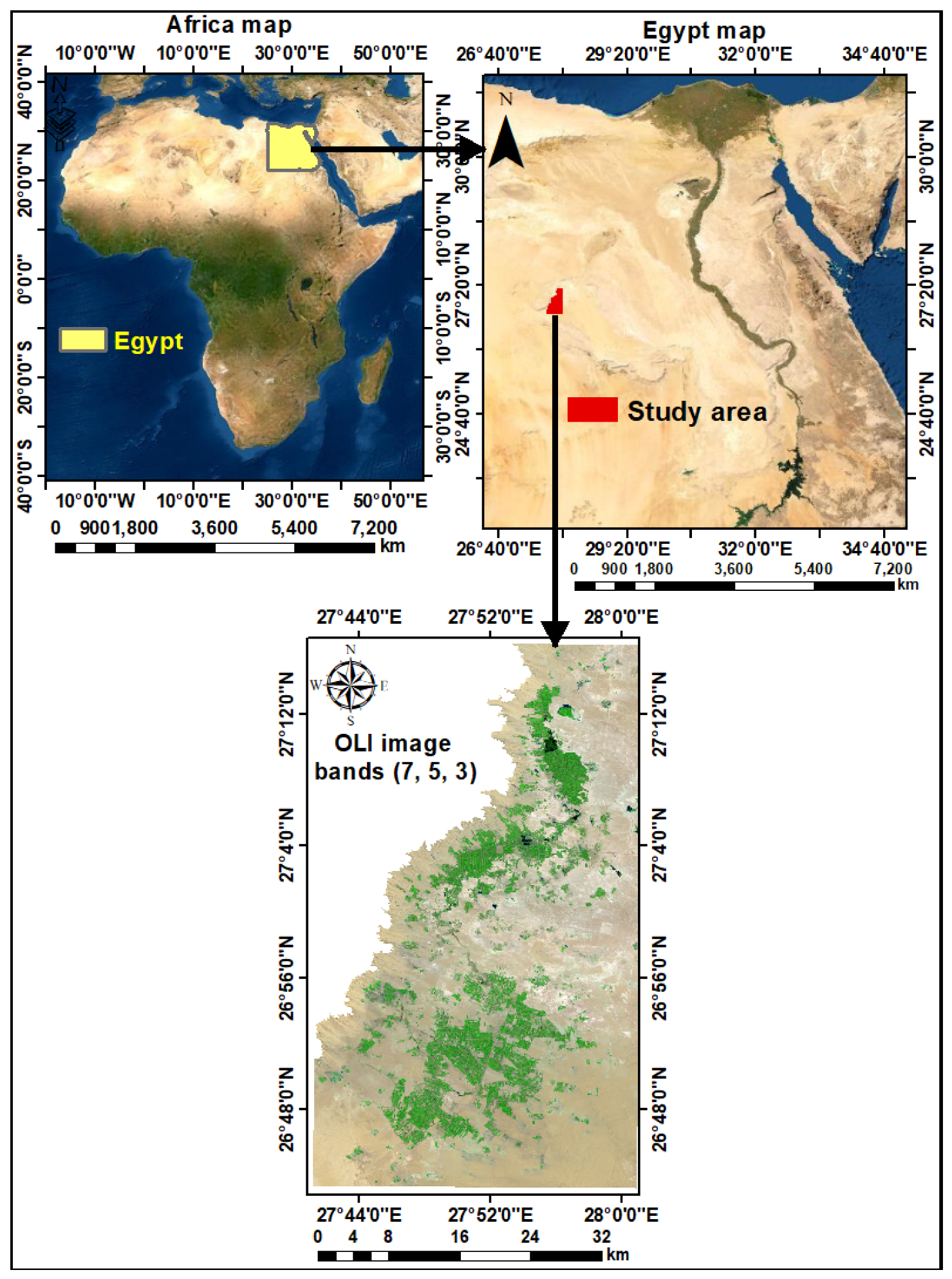
2.1. Area of Study

Farafra Oasis is located in the central part of the Egyptian Western Desert. The studied area (1445.66 km², i.e., 144,566 ha) is located in UTM zone 35 between latitudes 26°43′19″ to 27°16′23″ N and longitudes 27°41′14″ to 28°01′8″ E (Figure 1).

2.1.1. Climate

The climatic data (average of 15 years from 2005 to 2020) collected from El-Farafra station (latitude: 27°03′30″ N: longitude: 27°59′21″ E, elevation: 28.3 m) indicate that the minimum temperate is 4.9 °C and occurs during January, while the highest one is 38.5 °C and occurs during July. The mean annual temperature is 22.6 °C and the total annual rainfall is 21.4 mm. According to Soil Survey Staff [38], the soil temperature regime is Thermic and the soil moisture regime is Torric. The mean annual potential evapotranspiration (PET) is 3.5 mm day⁻¹. The area is a hyper-arid zone with an aridity index <0.01. The mean annual relative humidity averages 39.8%, while the mean annual wind speed is 10.4 km/h⁻¹.

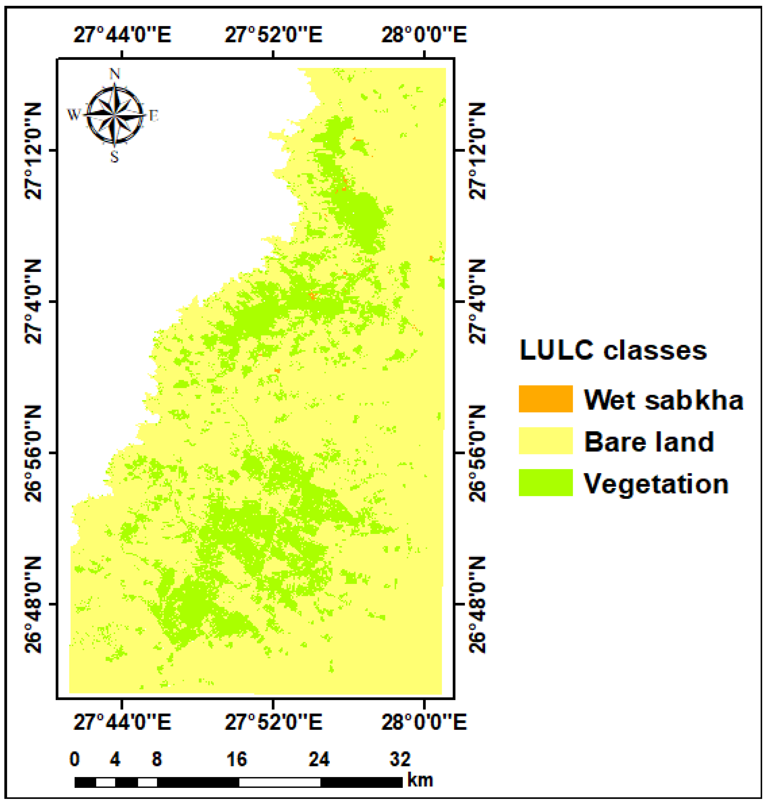
2.1.2. Land Use/Land Cover

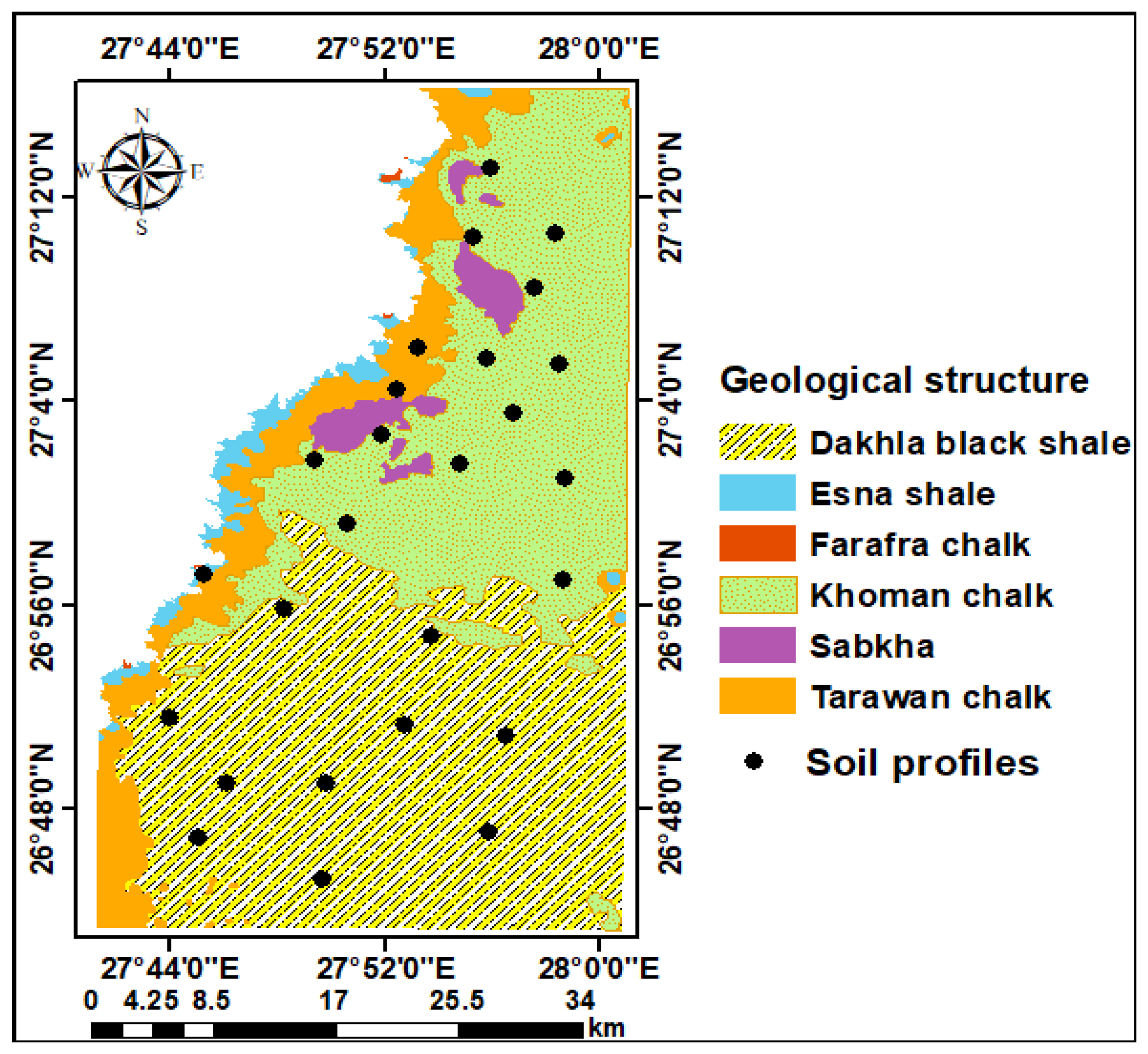
The area is dominated by three land use/land cover classes: bare land, vegetation (natural and cropland), and bare wet sabkha (Figure 2). These classes occupied 1223.30, 220.84, and 1.52 km², which represented 84.62%, 15.28%, and 0.10% of the total area, respectively. The natural vegetation occurred in scattered areas covered with halophytic species (Chenopodiaceae) around the sabkha. The croplands include field crops, orchards, and vegetable crops.

2.1.3. Geology

The geological map [39] shown in Figure 3 illustrates that the area is dominated by sedimentary sequences of Palaeocene, Eocene and Quaternary eras. The western parts of the area are dominated by Farafralimestones (lower Eocene), and chalky limestone of Paleocene (Tarawan Formation). The remaining parts are covered with Quaternary Formations (Sabkha), chalk of Upper Cretaceous (Dakhla and Khoman Formations).

2.2. Data Used

It is well known that LDV is affected by a wide range of factors [16,17,19], and thus, a range of evaluation criteria have been identified based on literature (

Table 1. Data characterizing land degradation vulnerability.

Index	Parameter	Class	Description	Score	Reference
Geology	Parent material	1	Shale, schist, basic, ultra-basic, Conglomerates, unconsolidate	0.1	[40]
		2	Limestone, marble, granite, Rhyolite, Ignibrite, gneiss, siltstone, sandstone	0.5
		3	Marl, Pyroclastics	1.0
Topography	Slope, %	1	Gently sloping: <5	0.1	[41]
		2	Sloping: 5–10	0.3
		3	Strongly sloping: 10–15	0.5
		4	Moderately steep: 15–30	0.6
		5	Steep: 30–60	0.8
		6	Very steep: >60	1.0
	Aspect	1	North	0.1	[42]
		2	South	0.3
		3	Flat	0.6
		4	East	0.8
		5	West	1.0
	Topographic wetness index (TWI)	1	Very high: >5	0.1
		2	High: 5–4	0.3
		3	Moderate: 4–3	0.6
		4	Low: 3–2	0.8
		5	Very low: <2	1.0
	Curvature	1	Liner: −0.1 to 0.1	0.2
		2	Convex: >0.1	0.5
		3	Concave: <−0.1	1.0
Physical soil quality	Depth, cm	1	Very deep: >150	0.1	[43]
		2	Deep: 150–100	0.3
		3	Moderately deep: 100–50	0.6
		4	Shallow: 50–30	0.8
		5	Very shallow: <30	1.0
	Gravel, %	1	Few: <5	0.1	[41]
		2	Common: 5–15	0.3
		3	Many: 15–40	0.6
		4	Abundant: 40–80	0.8
		5	Dominant: >80	1.0
	Texture	1	Clay	0.1	[30]
		2	Sandy clay, silty clay	0.3
		3	Sandy clay loam, silty clay loam, clay loam	0.6
		4	Sandy loam, loam, silt loam, silt	0.8
		5	Sand, loamy sand	1.0
	Bulk density (BD), Mg m−3	1	None: <1.2	0.1	[43]
		2	Slight: 1.2–1.4	0.3
		3	Moderate: 1.4–1.6	0.6
		4	Strong:1.6–1.8	0.8
		5	Extreme: >1.8	1.0
Chemical soil quality	pH	1	Neutral: 6.6–7.3	0.1	[44]
		2	Slightly alkaline: 7.4–7.8	0.3
		3	Moderately alkaline: 7.9–8.4	0.6
		4	Strongly alkaline: 8.5–9.0	0.8
		5	Very strongly alkaline: >9.0	1.0
	Electrical conductivity (EC), dS m−1	1	None: <4	0.1	[43]
		2	Slight: 4–8	0.3
		3	Moderate: 8–16	0.6
		4	Strong: 16–32	0.8
		5	Extreme: >32	1.0
	Exchangeable sodium percentage (ESP)	1	None: <10	0.1	[43]
		2	Slight: 10–15	0.3
		3	Moderate: 15–30	0.6
		4	Strong: 30–50	0.8
		5	Extreme: >50	1.0
	Organic matter (OM), g kg−1	1	Very high: >50	0.1	[30]
		2	High: 50–30	0.3
		3	Moderate: 30–17	0.6
		4	Low: 17–10	0.8
		5	Very low: <10	1.0
	CaCO3, g kg−1	1	Non-calcareous: 0 g	0.1	[41]
		2	Slightly calcareous: 0–20	0.3
		3	Moderately calcareous: 20–100	0.6
		4	Strongly calcareous: 100–250	0.8
		5	Extremely calcareous: >250	1.0
	Gypsum, g kg−1	1	Non-gepsiric: 0	0.1	[41]
		2	Slightly gypsiric: 0–50	0.3
		3	Moderately gypsiric: 50–150	0.6
		4	Strongly gypsiric: 150–600	0.8
		5	Extremely gypsiric: >600	1.0
Wind erosion	Climate erosivity factor (CE)	1	Very low: <20	0.1	[45]
		2	Low: 20–50	0.3
		3	Moderate: 50–70	0.6
		4	Severe: 70–100	0.8
		5	Extreme: >100	1.0
	Soil erodible fraction (EF), %	1	Very slight: <0.2	0.1	[46]
		2	Slight: 0.2–0.3	0.3
		3	Moderate: 0.3–0.4	0.6
		4	High: 0.4–0.5	0.8
		5	Very high: >0.5	1.0
	Surface crust factor (SCF) (dimensionless)	1	Very high: <0.1	0.1	[46]
		2	High: 0.1–0.3	0.3
		3	Moderate: 0.3–0.5	0.6
		4	Low: 0.5–0.7	0.8
		5	Very low: >0.7	1.0
	Surface roughness factor (SRF) (dimensionless)	1	Very high: <0.15	0.1	[47]
		2	High: 0.15–0.3	0.3
		3	Moderate: 0.3–0.5	0.6
		4	Low: 0.5–0.7	0.8
		5	Very low: >0.7	1.0
	Fractional vegetation cover (FVC) (dimensionless)	1	Very high density >0.8	0.1	[48]
		2	High density: 0.8–0.6	0.3
		3	Moderate density: 0.6–0.4	0.6
		4	Low density: 0.4–0.2	0.8
		5	Very low density: <0.2	1.0
Vegetation	NDVI	1	Very high: >0.6	0.1	[16]
		2	High: 0.6–0.5	0.3
		3	Moderate: 0.5–0.40	0.6
		4	Low: 0.4–0.3	0.8
		5	Very low: <0.3	1.0

). Data were collected from RS imageries, field observations, laboratory analyses, and climatic conditions.

Remote Sensing Data

One scene (path 178/row 41) of Landsat 8, Operational Land Imager (OLI) was acquired from the USGS Earth Explorer gateway (http://earthexplorer.usgs.gov/) on 10 January 2021. A Digital Elevation Model (DEM) with a 12.5 m pixel size of Advanced Land Observing Satellite (ALOS) Phased Array type L-band SAR (PALSAR) was also downloaded from the Alaska Satellite Facility (ASF) (https://www.asf.alaska.edu/sar-data/palsar/). Digital processing of satellite imageries was performed using ENVI 5.1 software, including atmospheric correction (FLASH module), stretching, band stacking, mosaicking, and spatial and spectral subsets. Thereafter, an unsupervised classification (ISO DATA classifier) followed by a supervised classification (maximum likelihood) was executed. The normalized difference vegetation index (NDVI) was calculated as follows:

$$\mathrm{NDVI}=\frac{\mathrm{NIR}\left(\mathrm{band}8\right) - \mathrm{RED}\left(\mathrm{band}4\right)}{\mathrm{NIR}\left(\mathrm{band}8\right) + \mathrm{RED}\left(\mathrm{band}4\right)}.$$

Within ArcGIS 10.8 (ESRI Co, Redlands, CA, USA), slope classes, aspect, topographic wetness index (TWI), and curvature were extracted from the DEM. The TWI was calculated according to Haghighi, Darabi [49] as follows:

$$\mathrm{TWI}=\mathrm{Ln}\left(\frac{{\mathrm{A}}_{\mathrm{s}}}{\tan \mathsf{\beta }}\right)$$

where A_s is the local upslope contributing area derived from flow accumulation raster and β is slope raster.

2.3. Field Work and Laboratory Analyses

Twenty-six geo-referenced soil profiles (Figure 2) were due to a 150 cm depth or lithic contact. General features of each profile were extensively observed according to FAO [41]. Ninety-three soil samples were collected from the subsequent horizons. Another set of undisturbed soil cores (100 cm³ volume) were collected from each depth to determine the soil bulk density (BD). At each depth, three replicates of 1 kg each were compiled in one composite sample, kept in polyethylene bags, and transported to the laboratory. Soil samples were air-dried, ground, passed through a 2-mm mesh, and kept for analyses. Soil analyses were performed according to the Soil Survey Staff [50]. The particle size distribution was carried out using the standard pipette method. The pH and EC were measured in the 1:2.5 soil-water suspension for the former and in the soil paste extract for the latter. Soil Organic matter (OM) was determined using the Walkley–Black procedure. The cation exchange capacity (CEC) and exchangeable sodium were determined using the ammonium acetate at pH = 7.0. Calcium carbonate was determined using the calcimeter, while gypsum content was determined using the acetone precipitation method.

2.4. Wind Erosion Calculation

The index of land susceptibility to wind erosion (ILSWE) developed by Fenta et al. [45] was used for estimating wind erosion severity as follows:

$$\mathrm{ILSWE}=\mathrm{CE}\times \mathrm{EF}\times \mathrm{SCF}\times \mathrm{VC}\times \mathrm{SR}$$

where CE is the climatic erosive factor, EF is the wind-erodible fraction factor, SCF is the soil crust factor, VC is the vegetation cover factor and SR is the surface roughness factor.

• Climatic Erosive Factor (CE)

The CE was calculated as follows:

$$\mathrm{E}=\raisebox{1ex}{$1$}\!\left/ \!\raisebox{-1ex}{$100$}\right.{\displaystyle \sum }_{\mathrm{i}=1}^{\mathrm{i}=12}{\mathrm{W}}_{\mathrm{i}}^3\left[\frac{{\mathrm{PET}}_{\mathrm{i}}-{\mathrm{P}}_{\mathrm{i}}}{{\mathrm{PET}}_{\mathrm{i}}}\right]\times {\mathrm{d}}_{\mathrm{i}}$$

where: W_i is the mean monthly wind speed (m s⁻¹) at 2 m height in month i, PET_i is the potential evapotranspiration (mm) in month i, P_i is the precipitation (mm) in a month i, and di is the total number of days in the month i.

• Wind-Erodible Fraction Factor (EF)

The EF was calculated as follows:

$$\mathrm{EF}=\frac{29.09+0.31\mathrm{SA}+0.17\mathrm{SI}+0.33\frac{\mathrm{SA}}{\mathrm{CL}}-2.59\mathrm{SOM}-0.95{\mathrm{CaCO}}_3}{100}$$

where EF is expressed in percent, SA is the sand content, SI is the silt content, CL is the clay content, OM is the organic matter content.

• Soil Crust Factor (SCF)

The SC factor was calculated as follows:

$$\mathrm{SCF}=\frac{1}{1+0:0066{\left(\mathrm{CL}\right)}^2+0.21{\left(\mathrm{OM}\right)}^2}$$

• Vegetation Cover Factor (VCF)

The VCF was expressed by the fractional vegetation cover (FVC) derived from the satellite image. The FVC was computed based on values of NDVI of highly dense vegetation (NDVIv) and bare soil (NDVIs) as follows:

$$\mathrm{FVC}=\frac{\mathrm{NDVI}-{\mathrm{NDVI}}_{\mathrm{s}}}{{\mathrm{NDVI}}_{\mathrm{v}}-{\mathrm{NDVI}}_{\mathrm{s}}}$$

• Surface Roughness Factor (SRF)

The SR was calculated based on the ratio of ridge height to ridge spacing, expressed as an index normally ranging from 0 (high ridges and furrows) to 1 (flat, bare, and smooth field) [51]. The SRF was calculated using the focal statics tools within ArcGIS 10.8 [45] as flows:

$$\mathrm{SRF}=\frac{{\mathrm{DEM}}_{\mathrm{Mean}}-{\mathrm{DEM}}_{\mathrm{Min}}}{{\mathrm{DEM}}_{\mathrm{Max}}-{\mathrm{DEM}}_{\mathrm{Min}}}$$

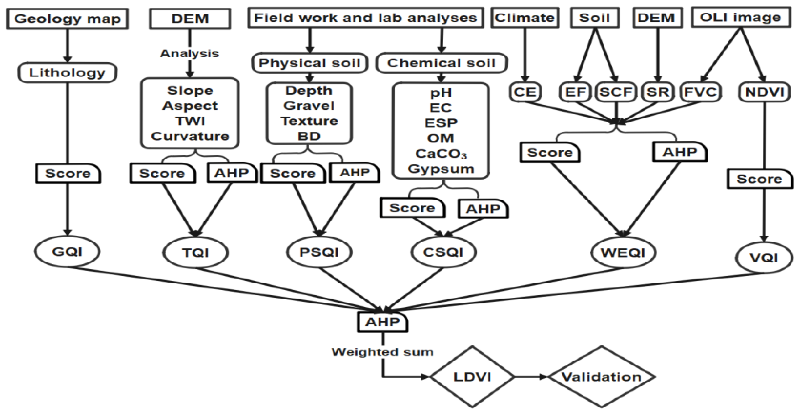
2.5. Modelling Land Degradation Vulnerability

This procedure implied five steps; (1) selecting the criteria, (2) assigning a rating for each criterion, (3) calculating a weight for each criterion, (4) developing five indices (topography, physical soil, chemical soil, wind erosion, and vegetation), and (5) generating the final LDV map.

• Selecting and Generating Thematic Layers of LDV Criteria

A thematic map layer of each criterion has been generated using GIS tools. Thereafter, each layer was given a score ranging from 0.1 to 1.0 (Table 1), where 0.1 was assigned to the lowest class pertaining to the specific LDV index, while 1.0 was assigned to the highest triggering class.

2.5.1. Generating LDV Indices

Six indices characterizing LDV have been developed; Geology index (GI), topographic quality index (TQI), physical soil quality index (PSQI), chemical soil quality index (CSQI) wind erosion quality index (WEQI), and vegetation quality index (VQI). For TQI, PSQI, CSQI, and WEQI, a pairwise comparison matrix was established, and then a comparison of each criterion to one another was done with a rating scale (1 ÷ 9) developed by Saaty [27]. Prioritizing the selected criteria according to their importance depended on literature, consulting local experts and stockholders (n = 10) throughquestionnaires, in addition to authors’ experiences. Hence, a weight value for each criterion was developed. In order to check the reality of the weights, the consistency ratio (CR) was considered, where CR values <0.10 indicate a real estimation, while CR values >0.10 require a revised judgment. After obtaining the weights, a thematic map for each index was generated using the weighted sum algorithm as follows:

$${\mathrm{Index}}_{\mathrm{x}}={\displaystyle \sum }_{\mathrm{i}=1}^{\mathrm{n}}{\mathrm{S}}_{\mathrm{i}}\times {\mathrm{W}}_{\mathrm{i}}$$

where S_i is the score value, W_i is the weight of the criteria and n is the number of criteria.

2.5.2. Geostatistical Analysis

The geostatistical analyst within ArcGIS tools was applied to predict and map soil attributes in unsampled areas using the ordinary kriging (OK) method. The OK is the most robust and common interpolation method [52,53]. The unsampled value Z (S0) is calculated by taking it as a linear combination of the neighboring observations as follows:

$$\mathrm{Z}\left({\mathrm{S}}_0\right) ={\displaystyle \sum }_{\mathrm{i}=1}^{\mathrm{N}}{\mathsf{\lambda }}_{\mathrm{i}}\times \mathrm{Z}({\mathrm{S}}_{\mathrm{i}})$$

where λ_i is the unknown weight for the measured value at the ith location, Z(S_i) is the measured value at the ith location, and N is the number of measured values. Within the OK method, various prediction models are used. However, spherical, exponential, and Gaussian are the most widely accepted used [53,54].

2.5.3. Generating the Final LDV Map

$$\mathrm{LDVI}= \left[\left(\mathrm{GI}\times {\mathrm{W}}_{\mathrm{i}}\right) + \left(\mathrm{TQI}\times {\mathrm{W}}_{\mathrm{i}}\right) + \left(\mathrm{PSQI}\times {\mathrm{W}}_{\mathrm{i}}\right) + \left(\mathrm{CSQI}\times {\mathrm{W}}_{\mathrm{i}}\right) + \left(\mathrm{WEQI}\times {\mathrm{W}}_{\mathrm{i}}\right) + \left(\mathrm{VQI}\times {\mathrm{W}}_{\mathrm{i}}\right)\right]$$

The LDVI was finally classified into five classes: very low (<0.2), low (0.2–0.4), moderate (0.4–0.6), high (0.6–0.8) and very high (>0.8). A flowchart of the methodology used in the current work is shown in Figure 4.

2.6. Model Validation

The model performance was checked considering two types of accuracies; the first one for the AHP based on CR, while the second step for data provided for generating LDV map. In the first step, the AHP was applied two times, considering the average and geometric mean algorithm of the expert opinions. The method with low CR was taken to the next step. In the second step, data were collected from satellite imageries, which were verified by field surveys. The cross-validation technique was performed to test geostatistical models used for predicting soil properties. Such a verification considered prediction errors, including mean error (ME), root means square error (RMSE), mean standardized error (MSE), root mean square standardized error (RMSSE), and average standardized error (ASE).

3. Results

3.1. Geology Index (GI)

As shown in Figure 2, the shale formations cover 731.11 km², representing 50.57% of the total area. Chalk carbonate rocks cover 674.16 km² and account for 46.64% of the total area. The sabkha formations were the least abundant and cover 40.39 km² that represent only 2.79% of the total area. Accordingly, nearly half of the total area was dominated by high-quality parent material (shale), 47% was dominated by moderate quality (chalk), while 3% was dominated by low quality (sabkha formations).

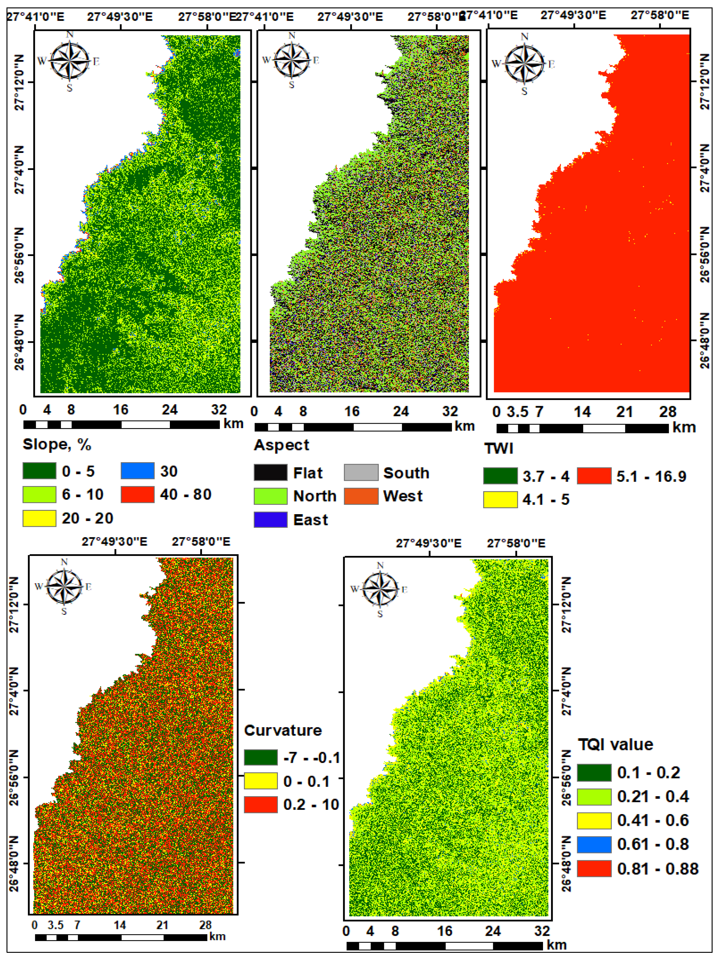
3.2. Topographic Quality Index (TQI)

The spatial distribution of topographic criteria (slope, aspect, TWI, curvature, and TQI) is presented in Figure 5. The DEM analysis indicates the slope gradient varied from 0 to 81%, indicating a flat to very steep slope gradient [41]. The aspect map demonstrates that slopes facing south (south, southeast, and southwest) and slope facing north (north, northeast, and northwest) dominated the studied area. Values of the TWI varied from 3.70 to 16.90, indicating a moderate to very high wetness degree [42]. The topographic curvature map ranged from −7.19 to 10.67. Areas of convex and concave surface dominated the studied area, while flat surface areas covered small parts. The results of the AHP (

Table 2. Pairwise comparison matrix for prioritize factor used.

Indices and Criteria within Each Index	Pair-Wise Comparison Matrix						Weight
	(1)	(2)	(3)	(4)	(5)	(6)
Index
(1) Geology	1	1/3	1/4	1/3	2	1/3	0.07
(2) Topography	3	1	1/3	1/3	3	1/2	0.12
(3) Physical soil quality	4	3	1	1	4	2	0.29
(4) Chemical soil quality	3	3	1	1	4	3	0.30
(5) Wind erosion quality	1/2	1/3	1/4	1/4	1	1/3	0.05
(6) Vegetation quality	3	2	1/2	1/3	3	1	0.17
Consistency ratio (CR)	0.04					Sum	1.00
Topographic quality criteria
(1) Slope	1	2	5	9			0.54
(2) Aspect	1/2	1	4	5			0.31
(3) TWI	1/5	1/4	1	2			0.10
(4) Curvature	1/9	1/5	1/2	1			0.06
Consistency ratio (CR)	0.011					Sum	1.00
Physical soil quality criteria
(1) Depth	1	2	4	8			0.52
(2) Gravel	1/2	1	3	5			0.30
(3) Texture	1/4	1/3	1	2			0.12
(4) Bulk density	1/8	1/5	1/2	1			0.06
Consistency ratio (CR)	0.006					Sum	1.00
Chemical soil quality criteria
(1) pH	1	1/4	1/3	1/2	1/3	2	0.07
(2) EC	4	1	2	5	4	6	0.40
(3) ESP	3	1/2	1	3	3	5	0.25
(4) OM	2	1/5	1/3	1	2	4	0.13
(5) CaCO3	3	1/4	1/3	1/2	1	3	0.11
(6) Gypsum	1/2	1/6	1/5	1/4	1/3	1	0.04
Consistency ratio (CR)	0.048					Sum	1.00
Wind erosion quality criteria
(1) Climate	1	4	5	9	2		0.46
(2) Soil erodibility	1/4	1	3	3	1/3		0.14
(3) Surface crust	1/5	1/3	1	2	1/4		0.07
(4) Surface roughness	1/9	1/3	1/2	1	1/4		0.05
(5) Vegetation cover	1/2	3	4	4	1		0.28
Consistency ratio (CR)	0.032					Sum	1.00

) indicate that slope was the most influence topographic feature (0.54) followed by aspect (0.31) and TWI (0.10), while curvature was the least effective (0.06). When combining the scores of the four variables with their weights, it is clear that the TQI varied from 0.1 to 0.88, indicating very high to very low-quality classes. The spatial distribution of quality grades (

Table 3. Spatial distribution of quality grades in the studied area.

Quality Index	Class	Quality	Area, km2	Area, %
Topography	1	Very high	511.89	35.41
	2	High	672.87	46.54
	3	Moderate	243.10	16.82
	4	Low	14.11	0.98
	5	Very low	3.69	0.26
Physical soil	1	Very high	0.00	0.00
	2	High	352.23	24.36
	3	Moderate	1053.04	72.84
	4	Low	0.00	0.00
	5	Very low	0.00	0.00
Chemical soil	1	Very high	0.00	0.00
	2	High	126.20	8.73
	3	Moderate	855.05	59.15
	4	Low	416.79	28.83
	5	Very low	7.23	0.50
Wind erosion	1	Very high	0.00	0.00
	2	High	0.00	0.00
	3	Moderate	132.07	9.14
	4	Low	1273.20	88.07
	5	Very low	0.00	0.00
Vegetation	1	Very high	0.97	0.07
	2	High	6.78	0.47
	3	Moderate	37.34	2.58
	4	Low	59.90	4.14
	5	Very low	1340.68	92.74
Reference term (Sabkha)			40.65	2.81

) shows that areas of high quality covered 46.54% of the total area, while the remaining area was dominated by very high (35.54%), moderate (16.82%), low (0.98%), and very low (0.26%) quality classes.

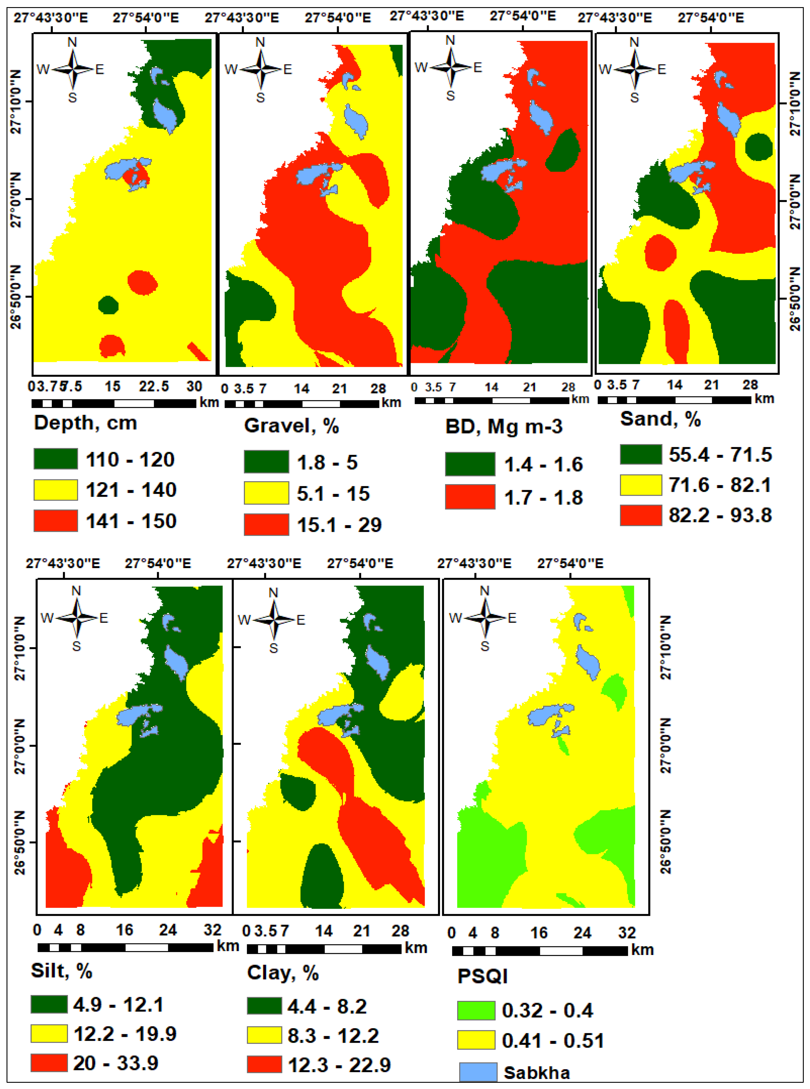
3.3. Physical Soil Quality Index (PSQI)

Maps of the physical soil attributes (effective depth, gravel content, texture, BD, and PSQI) are shown in Figure 6. The results illustrate that soil depth ranged from 110 to 150 cm, while the gravel content ranged from 1.8% to 29.0%. These results indicate a deep soil profile and a few to many gravel content [41]. The percentage ranges of sand, silt, and clay were 55.4% to 89.8%, 4.9% to 31.9%, and 4.4% to 22.9%, respectively. The sand dominated the soil particle size distribution averaging about 79% of the fine earth followed by silt (12%) and clay (9%). The soil BD varied from 1.4 to 1.8 Mg m⁻³, indicating moderate to strong compaction hazards [43]. The results of the AHP (Table 2) show that the maximum weight was assigned to effective soil depth (0.52) followed by gravel content (0.30), texture (0.12), and BD (0.06). The PSQI varied from 0.32 to 0.51, indicating high to moderate quality classes. The spatial analysis (Table 3) shows that the soils with a moderate physical quality degree covered 72.84% of the total area, while high physical quality soils occupied 24.36%.

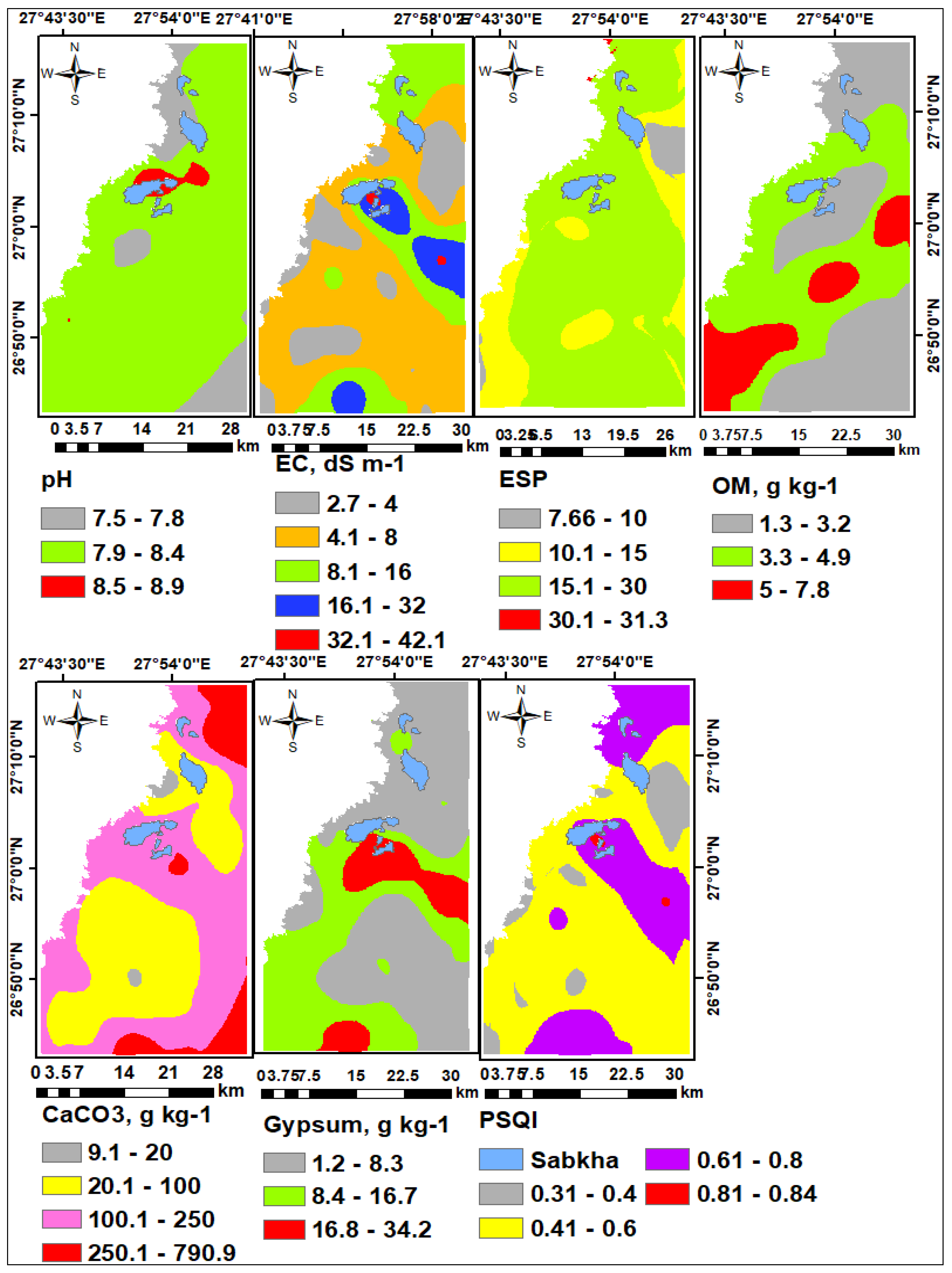
3.4. Chemical Soil Quality Index (CSQI)

The spatial distributions of chemical soil quality attributes (pH, EC, ESP, OM, CaCO₃, and gypsum) as presented in Figure 7. The soil pH ranged from 7.5 to 8.9, while the EC varied from 2.7 to 42.1 dS m⁻¹. These ranges indicate that the soils were slightly to strongly alkaline and non-saline to strongly saline [44]. The ESP varied from 7.7 to 31.3, indicating none to strong sodicity (alkalinity) hazards [43]. The soils had a very low OM content with a range of 1.3 to 7.8 g kg⁻¹. Calcium carbonate and gypsum contents varied from 9.1 to 790.9 g kg⁻¹ for the former and from 1.2 to 34.2 g kg⁻¹ for the latter. This indicates that the soils were moderate to extremely calcareous and slightly gypsiric [41]. The results of the AHP (Table 2) illustrate that EC had the highest weight (0.40) followed by ESP (0.25), OM (0.13), CaCO₃ (0.11), pH (0.07), and gypsum (0.04). The CSQI ranged from 0.32 to 0.84, which indicates a high to very low quality. The spatial analysis (Table 3) illustrates that moderate-quality soils occupied 59.15% of the total area, while high, low, and very low-quality soils covered 8.73%, 28.83%, and 0.50%, respectively.

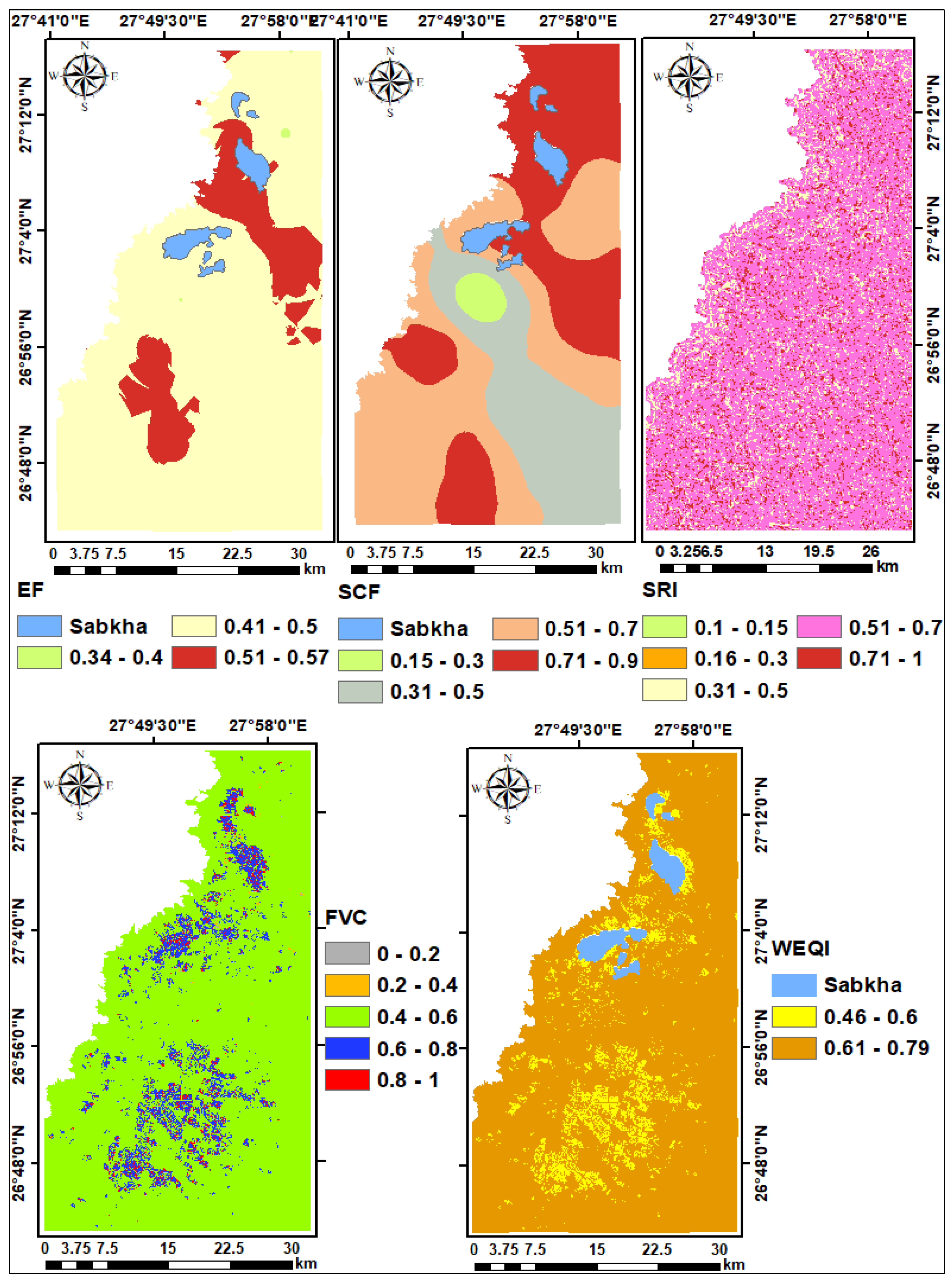
3.5. Wind Erosion Quality Index (WEQI)

The spatial distribution of the four input parameters determining wind erosion hazards is presented in Figure 8. The studied area is characterized by a moderate climate hazard with a CE value of 69.80, and thus the score value of CE was considered as 0.6 [45]. The EF values ranged from 0.34 to 0.57, indicating a moderate to very high soil erodibility [46]. The SCF varied from 0.15 to 0.89, which demonstrates a high to very low surface crust [46]. The SRF varied from 0.11 to 0.86, indicating a very high to very low surface roughness degree [47]. The FVC varied from 0 to 1.0, indicating a very low to very high vegetation density [48]. Results of the AHP show that CE was the most effective driver for wind erosion with a weight value of 0.46 followed by VCF (0.28), EF (0.14), SCF (0.07), and SRF (0.05). The WEQI varied from 0.46 to 0.79, indicating a moderate to low quality. The spatial distribution (Table 3) shows that 88.07% of the total area was under high erosion risks, while 9.14% was prone to moderate risks.

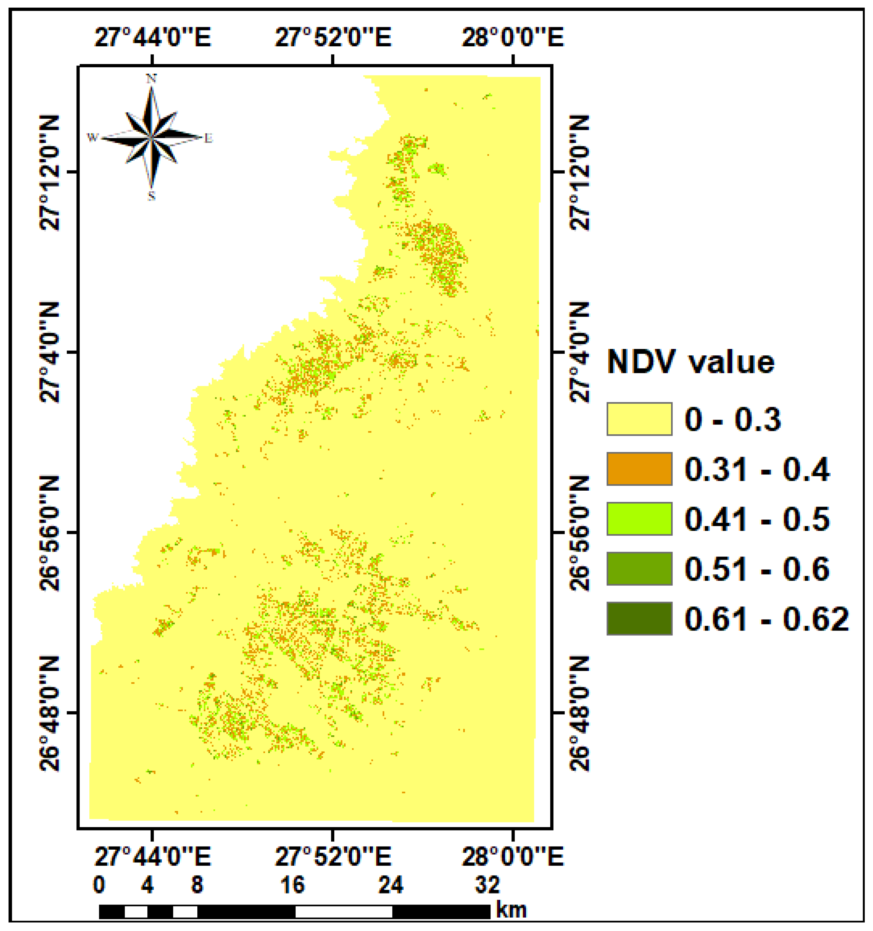
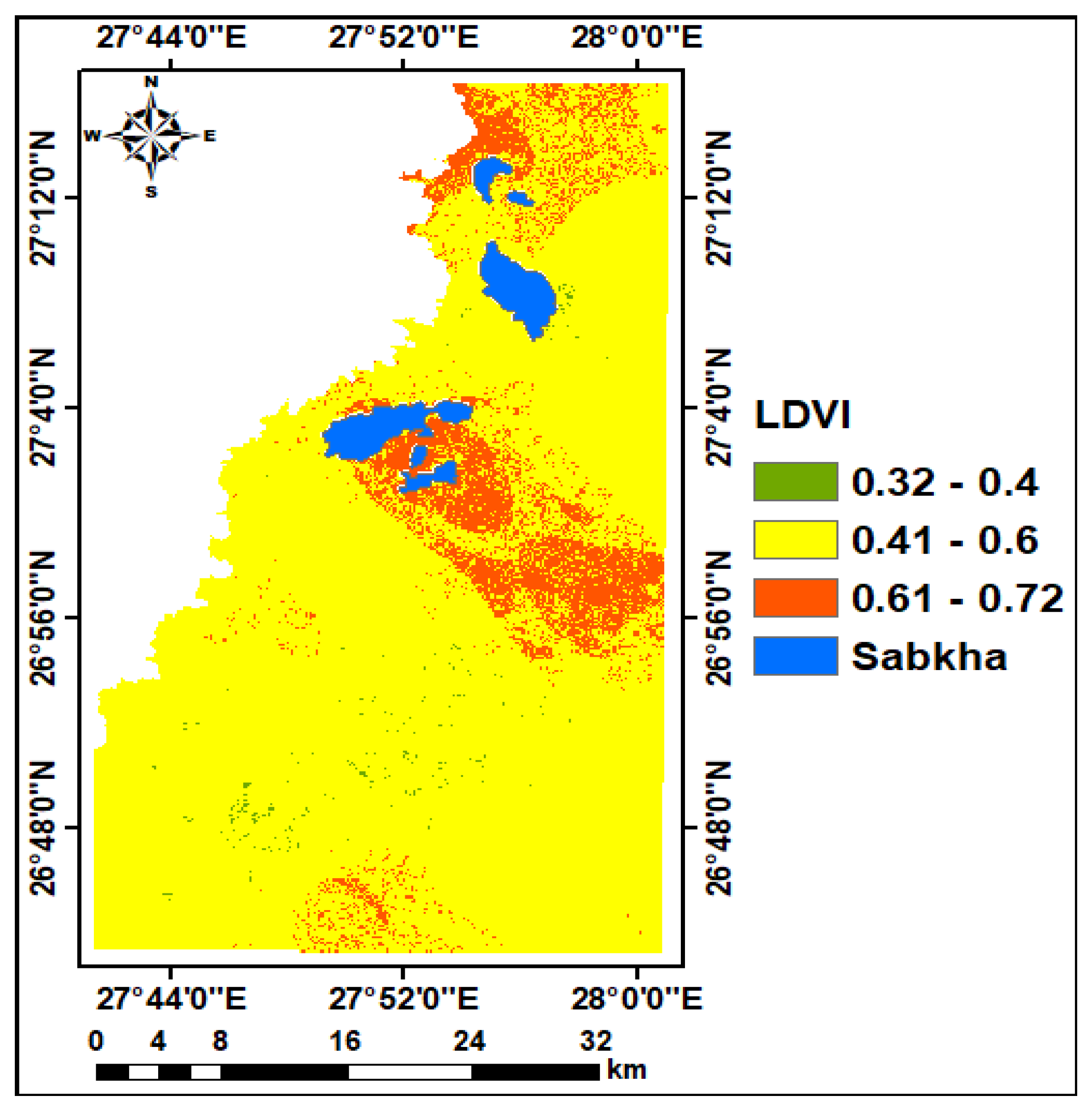
3.6. Vegetation Quality Index (VQI)

The VQI derived from the NDVI varied from 0.1 to 1.0, indicating a very high to very low quality [16]. The results in Figure 9 shows that the very low vegetation cover was the predominant class in the studied area and represented 92.74%. On the other hand, areas characterized by low, moderate, and high vegetation quality occupied 4.14%, 2.58%, and 0.47% of the total area, respectively. The very high vegetation cover was the least abundant class and represented only 0.07% of the total area.

3.7. The Overall LDV Map

The AHP (Table 2) illustrates that CSQI had the greatest priority in LDV with a weight value of 0.30 followed by PSQI (0.29), VQI (0.17), TQI (0.12), GI (0.07), while WEQI had the lowest effect with a weight value of 0.05. The LDVI map (Figure 10) demonstrates that values of LDVI varied from 0.32 to 0.72, indicating moderate to high degradation hazards. The spatial distribution (

Table 4. Spatial distribution of land degradation vulnerability classes in the studied area.

Class	Hazard Degree	Index Value	Area, km2	Area, %
1	Very low	<0.2	0.00	0.00
2	Low	0.2–0.4	7.24	0.50
3	Moderate	0.4–0.6	1232.98	85.29
4	High	0.6–0.8	164.80	11.40
5	Very high	>0.8	0.00	0.00
Reference term (Sabkha)			40.65	2.81
Total			1445.66	100.00

) illustrates that the studied area was vulnerable to low, moderate, and high degradation hazards. Moderate degradation hazards threatened 1232.98 km² that represents 85.29% of the total area. High degradation hazards affected 164.80 km², i.e., 11.40% of the total area. Areas were prone to low degradation hazards affected a small area (7.24 km²) that represented only 0.50% of the total area.

3.8. Validation

The results of the AHP (Table 2) show that values of the CR of all studied parameters and indices were less than 0.1. Cross-validation results (

Table 5. Cross-validation of prediction errors for ordinary kriging models.

Soil Property	Model	ME	RMSE	MSE	RMSSE	ASE
Depth	Gaussian	−0.014	12.390	0.002	1.038	12.072
Gravel	Exponential	0.091	5.466	−0.040	0.976	6.895
BD	Exponential	−0.002	0.096	−0.021	1.052	0.093
EC	Spherical	−0.073	11.929	−0.005	0.982	12.234
ESP	Gaussian	0.073	5.548	0.017	1.068	5.203
CaCO3	Gaussian	0.080	14.600	−0.030	1.160	15.640
Gypsum	Exponential	0.039	9.194	−0.021	1.080	8.339
EF	Exponential	0.004	0.073	0.039	0.930	0.078
SCF	Spherical	−0.005	0.021	−0.080	0.940	0.250
Sand	Exponential	−0.012	10.202	−0.008	0.948	10.818
Silt	Spherical	0.025	6.859	−0.035	1.028	6.649
Clay	Spherical	0.051	5.444	−0.070	1.094	5.540
pH	Spherical	−0.003	0.326	−0.019	1.067	0.306
OM	Exponential	−0.007	1.875	−0.009	1.018	1.818

) indicate that values of ME and MSE were close to 0, while values of RMSSE were close to 1.0. Moreover, the values of RMSE and ASE were rather similar. However, they showed higher values for most of the studied properties. The results also showed that the exponential model was suitable for six soil properties (gravel content, BD, gypsum content, EF, sand, and OM), followed by the spherical model that was proper to five properties (EC, SCF, silt, clay, and pH), and the Gaussian model that was suitable for only three properties (depth, ESP, and CaCO₃).

4. Discussion

4.1. Geology

Parent materials or local geology is an effective soil forming-factor, which plays an obvious role in soil development, especially under aridity conditions. The physicochemical properties of soil bedrock and the rates at which they are uplifted and weathered strongly affect soil properties [55]. Soils derived from different geological formations react differently to soil fertility, erosion, and vegetation [56]. In the studied area, nearly 50% of the soils are covered with shale, which is considered good parent materials [40]. Sedimentary rocks like shale contain sufficient basic cations like Ca²⁺, Na⁺, and K⁺ that provide a high capacity to supply mineral cations to plants [57]. On the other hand, about 47% of the soils are underlain by chalk limestone, which in turn is classified as moderate quality parent material [40]. Limestone usually produces shallow soils with relatively low moisture content and nutrient availability [56].

4.2. Topography

Topographic factors, including slope, aspect, curvature, and TWI play a great role in soil development, productivity, and resistance to various degradation processes [58,59]. In the studied area the slope and aspect were the most effective factor affecting topographic quality and comprised together 0.85 of the total weights. This result is in line with those obtained in previous works [42,58,59]. The slope and aspect showed a wide range, and hence the area showed a wide variation in TQI ranging from very high to very low. However, the topographic analysis indicated that the area would support sustainable agricultural production, where nearly 82% of the total area belonged to very high and high-quality classes.

4.3. Physical Soil Quality

The soils showed physical properties (depth, texture, gravel, and BD) typical for hyper-arid desert conditions, which have been reported in previous studies [7,60]. Under very dry conditions, physical weathering of bedrocks occurs well, while chemical weathering is negligible. Therefore, the resultant soil is usually covered with sand and coarse fragments that increase bulk density [61]. From the four physical properties, effective soil depth and gravel content had the greatest effect on physical quality with weight values of 0.52 and 0.30, respectively. Soil depth is a major constrain in hyper-arid environments due to the presence of highly-weathering resistant bedrock and high carbonate content that prevent complete eluviation, and thus delay the development of soil depth [56,61]. This results in waterlogging problems, especially with inadequate drainage systems [31]. Moreover, high gravel content has a negative effect on biomass production and soil moisture conservation [40]. Both depth and gravel content showed little variations, and thus the PSQI arranged in two quality classes; moderate (73%) and high (24%). Therefore, modern irrigation systems (sprinkler and drip) and establishing effective drainage networks are recommended for sufficient water supply and preventing potential waterlogging.

4.4. Chemical Soil Quality

The soil showed chemical properties (pH, EC, ESP, OM, CaCO₃, and gypsum) typical for the dryland ecosystems, where soil bedrocks and aridity play great effects on soil properties [62]. Sedimentary rocks (shale and limestone) underlain the studied are rich in basic cations (Ca²⁺, Mg²⁺, Na⁺, and K⁺), and thus, the soils tended to have high pH values [57]. Due to the low rainfall, the deep leaching of soluble salts, lime, and gypsum is limited, and thus, they accumulate in soils [56,61]. The soil also showed a very low OM content is due to low vegetation cover and biomass production [62]. Among six chemical soil properties, EC and ESP had the greatest contribution to chemical quality with weight values of 0.40, and 0.25, respectively. These results are in line with previous studies [4,12], which indicate that salinity and/or sodicity are the main chemical degradation process in the hyper-arid oases. Both EC and ESP showed wide ranges of salinity, and sodicity hazards, respectively. This made the CSQI varying from high to very low quality. The moderate and low-quality soils dominated nearly 60% and 29% of the total area, respectively. This requires an effective management strategy to mitigate potential risks. In this context, selecting salt-tolerant crops, establishing adequate drainage systems, and integrated soil and water management practices should be considered.

4.5. Wind Erosion Quality

The analysis of wind erosion factors (CE, EF, SCF, SR, and VCF) showed that the area is highly susceptible to wind erosion risks. This is a common phenomenon in dryland soils [62], especially under hyper-arid climates [4,12]. This is a result of high climate erosivity coupled with low vegetation cover and highly erodible soil fraction [45,46]. Scarce rainfall, high evapotranspiration rate, and high wind velocity aggravate climate erosivity [62]. Low clay and organic matter content in soils promote the detachment of soil particles due to wind action [63]. The absence of dense vegetation cover accelerates soil mass transport [42]. The CE, VCF, and EF were the most effective drivers for wind erosion in the studied area and comprised 0.88 of the total weights. Accordingly, high erosion risks threatened 88% of the total area, while 9% was prone to moderate risks. These findings are in agreement with those reported in the Egyptian National Action Program to Combat Desertification [64], where wind erosion hazards in the western desert oases vary between moderate and severe with an average soil loss rate varying from 4.5 to 66.9 Mg ha⁻¹ year⁻¹. Increasing the vegetation cover seems to be the most effective strategy for controlling wind erosion in the studied area.

4.6. Vegetation Quality

The NDVI has been known as an effective tool for identifying the greenness of the vegetation and patterns of green biomass [16]. The vegetation status in the studied area would be a major driver for land degradation, since low and very low vegetation quality classes occupied nearly 97% of the total area. On one hand, the bare land occupied nearly 85% of the total coverage. On the other hand (according to official statics), field crops dominated 69% of the total cultivated area of which a perennial crop (alfalfa) covers 15%, while annual crops (wheat, barely clover, broad bean, maize, sorghum, and groundnuts) cover 54%. The remaining cultivated area was occupied by orchards (19%); mango, date palm, guava, and vegetable crops (13%); potato, tomato, onion, and arugula. The annual field crops provide low plant cover that in turn accelerate soil erosion as the soils remain bare during the growing periods [40].

4.7. The Final LDV Map

The AHP shows that the soil chemical and physical qualities were the most effective drivers for LDV in the studied area, and represented together 0.59 of the total weights. As a result, the final LDVI showed a trend rather similar to that of the CSQI and PSQI, where areas prone to moderate degradation hazards occupied the majority of the total area (85%), while that prone to high risks occupied nearly 11%. This is logic because scarce rainfall under a hyper-arid climate makes the modifications of major soil limitation (depth, salinity, and alkalinity) more difficult [61,62].

4.8. Validation

When testing the model performance, it is clear that all values of CR (Table 2) were within the acceptable limit of lesser than 0.1 [27]. This, in turn, indicates that the pairwise comparison matrices of LDV indices had good stability and the calculated weights of all parameters and indices were consistent. The results of the cross-validation (Table 5) show that the OK method was suitable and reliable for predicting the spatial distribution of the studied soil properties. These findings were rather similar to those obtained by Aldabaa and Yousif [53], who reported that OK models (spherical, exponential, and Gaussian) were suitable for mapping soil properties of some desert soils near Toshka Lakes. Values of ME and MSE close to 0 illustrate that the predicted values are unbiased [53]. Moreover, values of RMSE close to 1.0 demonstrate that the standard error is accurate [52]. On the other hand, high values of RMSE and ASE suggest that the number of samples should be increased in further studies.

5. Conclusions

In the current work, a novel trial for modelling LDV in hyper-desert oases was conducted and applied within 144,566 ha in Farafra, an inland Western Desert Oases in Egypt. The model based on the integration of data collected from climate conditions, geological maps, remote sensing imageries, field observations and laboratory analyses with AHP is to be used under GIS environment. Six indices determining LDV were generated. Weights derived from the AHP showed that the most effective drivers for land degradation in the studied area were CSQI (0.30) followed by PSQI (0.29), VQI (0.17), TQI (0.12), GI (0.07), while WEQI were the least (0.05). The studied area belonged to three degradation vulnerability classes; low, moderate, and high. The areas susceptible to moderate risks occupied the majority of the total area (85%), while those prone to high and low risks occupied 11% and less than 1%, respectively. The CR for the studied parameters and indices were within the acceptable limit (<0.1), indicating the high accuracy of the pairwise comparisons. Moreover, prediction errors demonstrated that the performance of the geostatistical models was proper and reliable for predicting and mapping soil properties. The combined use of geospatial techniques and AHP would provide better estimation of the current degradation status in the desert oases. The proposed model is a starting point for sustainable agricultural planning in the newly-reclaimed desert oases, particularly in hyper-arid regions.

References

1. Cherlet, M.; Hutchinson, C.; Reynolds, J.; Hill, J.; Sommer, S.; Von Maltitz, G. World Atlas of Desertification; Publications Office of the European Union: Luxembourg, 2018. [Google Scholar]
2. Lucatello, S.; Huber-Sannwald, E. Sustainable development goals and drylands: Addressing the interconnection. In Stewardship of Future Drylands and Climate Change in the Global South: Challenges and Opportunities for the Agenda 2030; Lucatello, S., Huber-Sannwald, E., Espejel, I., Martínez-Tagüeña, N., Eds.; Springer International Publishing: Cham, Switzerland, 2020; pp. 27–40. [Google Scholar]
3. Barman, A.; Basak, N.; Narjary, B.; Mitran, T. Land degradation assessment using geospatial techniques. In Geospatial Technologies for Crops and Soils; Mitran, T., Meena, R.S., Chakraborty, A., Eds.; Springer: Singapore, 2021; pp. 421–453. [Google Scholar]
4. Fargette, M.; Loireau, M.; Sghaier, M.; Raouani, N.; Libourel, T. The future ofoases in North Africa through the prism of a systemic approach: Towards which type of viability and coviability? In Coviability of Social and Ecological Systems: Reconnecting Mankind to the Biosphere in an Era of Global Change: Vol. 2: Coviability Questioned by a Diversity of Situations; Barrière, O., Ed.; Springer International Publishing: Cham, Switzerland, 2019; pp. 19–59. [Google Scholar]
5. Ling, H.; Xu, H.; Fu, J.; Fan, Z.; Xu, X. Suitable oasis scale in a typical continental river basin in an arid region of China: A case study of the Manas River Basin. Quat. Int. 2013, 286, 116–125. [Google Scholar] [CrossRef]
6. Yang, R.; Su, Y.; Kong, J. Effect of tillage, cropping, and mulching pattern on crop yield, soil C and N accumulation, and carbon footprint in a desert oasis farmland. Soil Sci. Plant Nutr. 2017, 63, 599–606. [Google Scholar] [CrossRef] [Green Version]
7. Fadl, M.E.; Abuzaid, A.S. Assessment of land suitability and water requirements for different crops in Dakhla Oasis, Western Desert, Egypt. Int. J. Plant Soil Sci. 2017, 16, 1–16. [Google Scholar] [CrossRef] [Green Version]
8. Abuzaid, A.S.; Abdellatif, A.D. Integration of multivariate analysis and spatial modeling to assess agricultural potentiality in Farafra Oasis, Western Desert of Egypt. Egypt. J. Soil Sci. 2021, 61, 171–180. [Google Scholar]
9. Shalaby, A.; Khedr, H.S. Remote Sensing and GIS for Land Use/Land Cover Change Detection in Dakhla Oasis. In Sustainable Water Solutions in the Western Desert, Egypt: Dakhla Oasis; Iwasaki, E., Negm, A.M., Elbeih, S.F., Eds.; Springer International Publishing: Cham, Switzerland, 2021; pp. 145–159. [Google Scholar]
10. Mohamed, S.H.I. The Egyptian Western Desert: Water, agriculture and culture of oasis communities. In Sustainable Water Solutions in the Western Desert, Egypt: Dakhla Oasis; Iwasaki, E., Negm, A.M., Elbeih, S.F., Eds.; Springer International Publishing: Cham, Switzerland, 2021; pp. 13–26. [Google Scholar]
11. Corti, G.; Cocco, S.; Hannachi, N.; Cardelli, V.; Weindorf, D.; Marcellini, M.; Agnelli, A. Assessing geomorphological and pedological processes in the genesis of pre-deserts oils from southern Tunisia. CATENA 2020, 187, 104290. [Google Scholar] [CrossRef]
12. Pei, H.; Fang, S.; Lin, L.; Qin, Z.; Wang, X. Methods and applications for ecological vulnerability evaluation in a hyper-arid oasis: A case study of the Turpan Oasis, China. Environ. Earth Sci. 2015, 74, 1449–1461. [Google Scholar] [CrossRef] [Green Version]
13. Elbeih, S.F.; Zaghloul, E.A. Hydrologeological and hydrological conditions of Dakhla Oasis. In Sustainable Water Solutions in the Western Desert, Egypt: Dakhla Oasis; Iwasaki, E., Negm, A.M., Elbeih, S.F., Eds.; Springer International Publishing: Cham, Switzerland, 2021; pp. 185–201. [Google Scholar]
14. Liu, X.X.; Xie, Y.; Zhou, D.; Li, X.; Ding, J.; Wu, X.; Wang, J.; Hai, C. Soil grain-size characteristics of Nitrariatangutorum Nebkhas with different degrees of vegetation coverage in a Desert-Oasis ecotone. Pol. J. Environ. Stud. 2020, 29, 3703–3714. [Google Scholar] [CrossRef]
15. King, C.; Thomas, D.S.G. Monitoring environmental change and degradation in the irrigated oases of the Northern Sahara. J. Arid Environ. 2014, 103, 36–45. [Google Scholar] [CrossRef]
16. Sandeep, P.; Reddy, G.P.O.; Jegankumar, R.; Kumar, K.C.A. Modeling and Assessment of Land Degradation Vulnerability in Semi-arid Ecosystem of Southern India Using Temporal Satellite Data, AHP and GIS. Environ. Model. Assess. 2021, 26, 143–154. [Google Scholar] [CrossRef]
17. Parmar, M.; Bhawsar, Z.; Kotecha, M.; Shukla, A.; Rajawat, A.S. Assessment of land degradation vulnerability using geospatial technique: A case study of Kachchh District of Gujarat, India. J. Indian Soc. Remote Sens. 2021. [Google Scholar] [CrossRef]
18. AbdelRahman, M.A.E.; Shalaby, A.; Aboelsoud, M.H.; Moghanm, F.S. GIS spatial model based for determining actual land degradation status in Kafr El-SheikhG overnorate, North Nile Delta. Model. Earth Syst. Environ. 2018, 4, 359–372. [Google Scholar] [CrossRef]
19. AbdelRahman, M.A.E.; Tahoun, S. GIS model-builder based on comprehensive geostatistical approach to assesss oil quality. Remote Sens. Appl. Soc. Environ. 2019, 13, 204–214. [Google Scholar]
20. Hereher, M.; El-Kenawy, A. Assessment of land degradation in northern Oman using geospatial techniques. Earth Syst. Environ. 2021. [Google Scholar] [CrossRef]
21. Turan, İ.D.; Dengiz, O.; Özkan, B. Spatial assessment and mapping of soil quality index for desertification in the semi-arid terrestrial ecosystem using MCDM in interval type-2 fuzzy environment. Comput. Electron. Agric. 2019, 164, 104933. [Google Scholar] [CrossRef]
22. Abuzaid, A.S.; Bassouny, M.A. Multivariate and spatial analysis of soil quality in Kafr El-Sheikh Governorate, Egypt. J. Soil Sci. Agric. Eng. Mansoura Univ. 2018, 9, 333–339. [Google Scholar] [CrossRef]
23. Jahin, H.S.; Abuzaid, A.S.; Abdellatif, D.A. Using multivariate analysis to develop irrigation water quality index for surface water in Kafr El-Sheikh Governorate, Egypt. Environ. Technol. Innov. 2020, 17, 100532. [Google Scholar] [CrossRef]
24. Abuzaid, A.S.; Jahin, H.S. Profile distribution and source identification of potentially toxic elements in north Nile Delta, Egypt. Soil Sediment Contam. Int. J. 2019, 28, 582–600. [Google Scholar] [CrossRef]
25. Sutadian, A.D.; Muttil, N.; Yilmaz, A.G.; Perera, B. Using the Analytic Hierarchy Process to identify parameter weights for developing a water quality index. Ecol. Indic. 2017, 75, 220–233. [Google Scholar]
26. Saaty, T.L. The Analytic Hierarchy Process; McGraw-Hill: New York, NY, USA, 1980. [Google Scholar]
27. Saaty, T.L. Decision Making with the Analytic Hierarchy Process. Int. J. Serv. Sci. 2008, 1, 83–98. [Google Scholar]
28. Kacem, H.A.; Fal, S.; Karim, M.; Alaoui, H.M.; Rhinane, H.; Maanan, M. Application of fuzzy analytical hierarchy process for assessment of desertification sensitive areas in North West of Morocco. Geocarto Int. 2021, 36, 563–580. [Google Scholar] [CrossRef]
29. Bakr, N.; Bahnassy, M.H. Land use/land cover and vegetation status. In The Soils of Egypt; El-Ramady, H., Alshaal, T., Bakr, N., Elbana, T., Mohamed, E., Belal, A.A., Eds.; Springer International Publishing: Cham, Switzerland, 2019; pp. 51–67. [Google Scholar]
30. Abuzaid, A.S.; Abdellatif, A.D.; Fadl, M.E. Modeling soil quality in Dakahlia Governorate, Egypt using GIS techniques. Egypt. J. Remote Sens. Space Sci. 2021, 24, 255–264. [Google Scholar] [CrossRef]
31. Abuzaid, A.S. Assessing degradation of Flood Plain soils in north east Nile Delta, Egypt. Egypt. J. Soil Sci. 2018, 58, 135–146. [Google Scholar]
32. Shihab, T.H.; Al-hameedawi, A.N. Desertification hazard zonation in central Iraq using multi-criteria evaluation and GIS. J. Indian Soc. Remote Sens. 2020, 48, 397–409. [Google Scholar] [CrossRef]
33. Wang, J.; Liu, D.; Ma, J.; Cheng, Y.; Wang, L. Development of a large-scale remote sensing ecological index in arid areas and its application in the Aral Sea Basin. J. Arid Land 2021, 13, 40–55. [Google Scholar] [CrossRef]
34. Bakr, N.; Weindorf, D.; Bahnassy, M.H.; El-Badawi, M.M. Multi-temporal assessment of land sensitivity to desertification in a fragilea gro-ecosystem: Environmental indicators. Ecol. Indic. 2012, 15, 271–280. [Google Scholar] [CrossRef]
35. Mohamed, E.S. Spatial assessment of desertification in north Sinai using modified MEDLAUS model. Arab. J. Geosci. 2013, 6, 4647–4659. [Google Scholar] [CrossRef]
36. Gad, A. Remotely sensed data for assessment of land degradation aspects, emphases on Egyptian case studies. In Sustainable Energy Investment—Technical, Market and Policy Innovations to Address Risk; Nyangon, J., Byrne, J., Eds.; IntechOpen: London, UK, 2021; pp. 181–201. [Google Scholar] [CrossRef]
37. Haidara, I.; Tahri, M.; Maanan, M.; Hakdaoui, M. Efficiency of Fuzzy Analytic Hierarchy Process to detect soil erosion vulnerability. Geoderma 2019, 354, 113853. [Google Scholar] [CrossRef]
38. Soil Survey Staff. Keys to Soil Taxonomy, 12th ed.; USDA-Natural Resources Conservation Service: Washington, DC, USA, 2014.
39. EGPC/CONCO-Coral. Geologic Map of Egypt, Scale 1:500000, Cairo, Egypt; EGPC/CONCO-Coral: Cairo, Egypt, 1987. [Google Scholar]
40. Kosmas, C.; Ferrara, A.; Briasouli, H.; Imeson, A. Methodology form appling environmentally sensitive areas (ESAS) to desertification. In The Medalus Project: Mediterranean Desertification and Land Use. Manual on Key Indicators of Desertification and Mapping Environmentally Sensitive Areas to Desertification; Kosmas, C., Kirkby, M., Geeson, N., Eds.; EUR18882; Office for Official Pubolications of the European Communities: Luxembourg, 1999. [Google Scholar]
41. FAO. Guidelines for Soil Description; FAO: Rome, Italy, 2006. [Google Scholar]
42. Sharma, T.; Singh, O. Soil erosion susceptibility assessment through geo-statistical multivariate approach in Panchkula district of Haryana, India. Model. Earth Syst. Environ. 2017, 3, 733–753. [Google Scholar] [CrossRef]
43. FAO. A Provisional Methodology for Soil Degradation Assessment; FAO: Rome, Italy, 1980. [Google Scholar]
44. Soil Science Division Staff. Soil Survey Manual. USDA Handbook 18; Government Printing Office: Washington, DC, USA, 2017.
45. Fenta, A.A.; Tsunekawa, A.; Haregeweyn, N.; Poesen, J.; Tsubo, M.; Borrelli, P.; Panagos, P.; Vanmaercke, M.; Broeckx, J.; Yasuda, H.; et al. Land susceptibility to water and wind erosion risks in the East Africa region. Sci. Total Environ. 2020, 703, 135016. [Google Scholar] [CrossRef]
46. Borrelli, P.; Ballabio, C.; Panagos, P.; Montanarella, L. Wind erosion susceptibility of European soils. Geoderma 2014, 234, 471–478. [Google Scholar] [CrossRef]
47. Mandakh, N.; Tsogtbaatar, J.; Dash, D.; Khudulmur, S. Spatial assessment of soil wind erosion using WEQ approach in Mongolia. J. Geogr. Sci. 2016, 26, 473–483. [Google Scholar] [CrossRef] [Green Version]
48. Zhang, S.; Chen, H.; Fu, Y.; Niu, H.; Yang, Y.; Zhang, B. Fractional vegetation covere stimation of different vegetation types in the Qaidam basin. Sustainability 2019, 11, 1–17. [Google Scholar]
49. Bernard, J.; Bocher, E.; Petit, G.; Palominos, S. (2018) Sky view factor calculation in urban context: Computational performance and accuracy analysis of two open and free GIS tools. Climate 2018, 6, 60. [Google Scholar] [CrossRef] [Green Version]
50. Soil Survey Staff. Soil Survey Field and Laboratory Methods Manual. Soil Survey Investigations Report No. 51, Version 2.0; Burt, R., Ed.; Department of Agriculture, Natural Resources Conservation Service: Washington, DC, USA, 2014.
51. Jarrah, M.; Mayel, S.; Tatarko, J.; Funk, R.; Kuka, K. A review of wind erosio nmodels: Data requirements, processes, and validity. Catena 2020, 187, 104388. [Google Scholar] [CrossRef]
52. Zhen, J.; Pei, T.; Xie, S. Kriging methods with auxiliary night time lights data to detect potentially toxic metals concentrations in soil. Sci. Total Environ. 2019, 659, 363–371. [Google Scholar] [CrossRef] [PubMed]
53. Aldabaa, A.A.A.; Yousif, I.A.H. Geostatistical approach for land suitability assessment of some desert soils. Egypt. J. Soil Sci. 2020, 60, 195–209. [Google Scholar] [CrossRef]
54. Mousavifard, S.M.; Momtaz, H.; Sepehr, E.; Davatgar, N.; Sadaghiani, M.H.R. Determining and mapping some soil physico-chemical properties using geostatistical and GIS techniques in the Naqade region, Iran. Arch. Agron. Soil Sci. 2013, 59, 1573–1589. [Google Scholar] [CrossRef]
55. Ben Mahmoud, K.R.; Zurqani, H.A. Soil forming factors and processes. In The Soils of Libya; Zurqani, H.A., Ed.; Springer International Publishing: Cham, Switzerland, 2021; pp. 33–48. [Google Scholar]
56. Osman, K.T. Factors and Processes of Soil Formation. In Soils: Principles, Properties and Management; Osman, K.T., Ed.; Springer: Dordrecht, The Netherlands, 2013; pp. 17–30. [Google Scholar]
57. Chapin, F.S.; Matson, P.A.; Vitousek, P.M. Geology, soils, and sediments. In Principles of Terrestrial Ecosystem Ecology; Chapin, F.S., Matson, P.A., Vitousek, P.M., Eds.; Springer: New York, NY, USA, 2011; pp. 63–90. [Google Scholar]
58. John, K.; Afu, S.M.; Isong, I.A.; Aki, E.E.; Kebonye, N.M.; Ayito, E.O.; Chapman, P.A.; Eyong, M.O.; Penížek, V. Mapping soil properties with soil-environmental covariates using geostatistics and multivariate statistics. Int. J. Environ. Sci. Technol. 2021. [Google Scholar] [CrossRef]
59. Haghighi, A.T.; Darabi, H.; Karimidastenaei, Z.; Davudirad, A.A.; Rouzbeh, S.; Rahmati, O.; Sajedi-Hosseini, F.; Klöve, B. Land degradation risk mapping using topographic, human-induced, and geo-environmental variables and machine learning algorithms, for the Pole-Doab watershed, Iran. Environ. Earth Sci. 2020, 80, 1. [Google Scholar] [CrossRef]
60. Abuzaid, A.S.; Fadl, M.E. Land evaluation of eastern Suez Canal, Egypt using remote sensing and GIS. Egypt. J. Soil Sci. 2016, 56, 537–548. [Google Scholar]
61. Blume, H.-P.; Brümmer, G.W.; Fleige, H.; Horn, R.; Kandeler, E.; Kögel-Knabner, I.; Kretzschmar, R.; Stahr, K.; Wilke, B.M. Soil development and soil classification. In Scheffer/Schachtschabel Soil Science; Blume, H.-P., Brümmer, G.W., Fleige, H., Horn, R., Kandeler, E., Kögel-Knabner, I., Kretzschmar, R., Stahr, K., Wilke, B.-M., Eds.; Springer: Berlin/Heidelberg, Germany, 2016; pp. 285–389. [Google Scholar]
62. Osman, K.T. Drylan soils. In Management of Soil Problems; Osman, K.T., Ed.; Springer International Publishing: Cham, Switzerland, 2018; pp. 15–36. [Google Scholar]
63. Guo, Z.; Chang, C.; Wang, R.; Li, J. Comparison of different methods to determine wind-erodible fraction of soil with rock fragments under different tillage/management. Soil Tillage Res. 2017, 168, 42–49. [Google Scholar] [CrossRef]
64. Desert Research Center (DRC). Egyptian National Action Program to Combat Desertification; DRC, Ministry of Agriculture and Land Reclamation (MALR): Cairo, Egypt, 2005. [Google Scholar]
Figure 1. Location: maps of the studied area.
Agronomy 11 01426 g001
Figure 2. Land use/land cover map of the studied area.
Agronomy 11 01426 g002
Figure 3. Geological map and soil profile locations in the studied area.
Agronomy 11 01426 g003
Figure 4. A flowchart of the proposed methodology in the current work.
Agronomy 11 01426 g004
Figure 5. Maps of topographic criteria in the studied area.
Agronomy 11 01426 g005
Figure 6. Maps of physical soil criteria in the studied area.
Agronomy 11 01426 g006
Figure 7. Maps of chemical soil criteria in the studied area.
Agronomy 11 01426 g007
Figure 8. Maps of wind erosion criteria in the studied area.
Agronomy 11 01426 g008
Figure 9. Map of vegetation quality index in the studied area.
Agronomy 11 01426 g009
Figure 10. Land degradation vulnerability map in the studied area.
Agronomy 11 01426 g010