Climate Projections for Precipitation and Temperature Indicators in the Douro Wine Region: The Importance of Bias Correction

Abstract

The implications of weather and climate extremes on the viticulture and winemaking sector can be particularly detrimental and acquire more relevance under a climate change context. A four-member ensemble of the Regional Climate Model-Global Climate Model chain simulations is used to evaluate the potential impacts of climate change on indices of extreme temperature and precipitation, as well as on agroclimatic indices of viticultural suitability in the Douro Wine Region, Portugal, under current and future climate conditions, following the RCP8.5 anthropogenic radiative forcing scenario. Historical (1989–2005) and future (2051–2080) periods are considered for this purpose. Although model outputs are bias-corrected to improve the accuracy of the results, owing to the sensitivity of the climatic indicators to the specific bias correction method, the performance of the linear and quantile mapping methods are compared. The results hint at the importance of choosing the most accurate method (quantile mapping), not only in replicating extremes events but also in reproducing the accumulated agroclimatic indices. Significant differences between the bias correction methods are indeed found for the number of extremely warm days (maximum temperature > 35 °C), number of warm spells, number of warm spell days, number of consecutive dry days, the Dryness Index, and growing season precipitation. The Huglin Index reveals lower sensitivity, thus being more robust to the choice of the method. Hence, an unsuitable bias correction method may hinder the accuracy of climate change projections in studies heavily relying on derived extreme indices and agroclimatic indicators, such as in viticulture. Regarding the climate change signal, significant warming and drying trends are projected throughout the target region, which is supported by previous studies, but also accompanied by an increase of intensity, frequency, and duration of extreme events, namely heatwaves and dry spells. These findings thereby corroborate the need to adopt timely and effective adaptation strategies by the regional winemaking sector to warrant its future sustainability and enhance climate resilience.

1. Introduction

Climate change is considered a major threat to the whole Earth’s climate system, its components and interactions [1]. During the last decades, not only has the mean temperature increased but the extremely high-temperature events have also intensified [2,3,4,5,6]. Since the mid-20th century, changes in extreme events have been observed worldwide and have been extensively reported by the scientific community [1]. Among such events, temperature and precipitation extremes tend to be particularly meaningful, owing to the critical role played by these two atmospheric elements on a wide spectrum of natural systems and socio-economic sectors. An overall decrease in the frequency of occurrence of cold spells, accompanied by an upward trend in the occurrence of warm spells, a strengthening of drought duration and intensity, as well as an intensification of heavy precipitation events have been documented [1]. Furthermore, for the upcoming decades, under different anthropogenic radiative forcing scenarios, with a range of greenhouse gas emission pathways, a reduction in the number of cold spells should be expected [7], while heat waves are projected to last longer, to be more intense, and to gradually cover larger areas [8,9]. However, changes in the extremes of minimum temperatures are expected to be more pronounced than in maximum temperatures [10].

For the Iberian Peninsula, in particular, several studies based on observational data demonstrated a downward trend in the amount of extreme precipitation in the last decades [11], while other studies report the opposite [12,13]. This discrepancy may be due to both different definitions of extreme events among the different studies (the results are very sensitive to their actual definition) and/or to the unequal spatial resolution of the original datasets, as these extremes can have strong spatial variability. In the future, an overall decrease in precipitation is expected over the Iberian Peninsula [14,15]. Nonetheless, extreme events are projected to have a higher contribution to the annual accumulated precipitation, in association with longer dry periods driven by strong anticyclonic ridges over the Eastern North Atlantic [16,17,18,19]. In terms of extreme temperatures, the results provided by several studies are much more consensual, evidencing that the number, duration, and intensity of heatwaves are expected to increase over the Iberian Peninsula [20,21,22,23]. It is also expected that the majority of the summer season will be under heatwave conditions [20]. Extreme heatwaves are also expected to increase, with some regions of the Iberian Peninsula experiencing more than 10 heatwave days with maximum temperatures over 45 °C [20]. The Iberian Peninsula is, thus, commonly considered as a ‘hot spot’ of climate change, whereas major socioeconomic systems operating in the region are strongly exposed and vulnerable to this threat, namely the agricultural sector [24].

More specifically for the viticultural sector and the wine production chain, the environmental conditions play a critical role by controlling yields and grape quality attributes, and ultimately the wine profiles, being a central component of the terroir of a given region [25]. The atmospheric conditions do have an important impact on grapevine development, as it requires specific ecoclimatic niches for its optimum development and growth, namely adequate temperatures, radiation intensity and duration, relative humidity, and levels of soil water availability during each specific phase of its vegetative and reproductive cycles [26].

Temperature is, indeed, the major driver of vine phenology [27], highlighting the strong sensitivity of this crop to atmospheric conditions and its resulting vulnerability to climate variability and change. Among many potential impacts in future climates, grapevines may be exposed to excessively high temperatures during the very sensitive grape berry ripening period [28], thus negatively affecting several physiological processes and, as a consequence, berry quality [29]. Extremely high temperatures often associated with intense radiation levels and water stress may also lead to heat sunburns in leaves and berries, with obvious negative implications in grapevine development, yield, and berry quality attributes [26]. Precipitation also plays an important role in grape berry quality. Moderate water deficits may have a positive effect on red wine quality, since the synthesis of grape skin phenolic compounds tends to increase [30,31], and wines tend to develop more complex aromas during bottle ageing [32,33]. Nevertheless, severe or extreme droughts often play a detrimental two-fold effect, combining anomalously low precipitation accumulation over a given period (precipitation deficit) with strengthened evapotranspiration caused by typically dry and warm air masses, thus resulting in severe soil water deficits. These deficits may have a strong impact on berry size and can thereby lead to lower yields [30] and diminished bud fertility [34]. Although not exhaustive, the aforementioned potential effects of temperature and precipitation extremes on grapevines are illustrative of the exposure and vulnerability of this crop to climate change and extremes.

The impacts of these atmospheric variables on grapevines can be better assessed through several agro-climatic indices, since they can provide a closer relationship between the weather conditions and the grapevine development, by integrating plant–atmosphere interactions [26]. These agro-climatic indices can also be used to assess the suitability of a given region for viticulture. Two very common indices used in viticultural zoning are the dryness index and the Huglin index [35]. While the dryness index is based on an estimation of the potential soil water balance, the Huglin index remits for the level of potential heliothermic capacity during the growing season, including a daylength coefficient.

Owing to the climatic changes projected for global temperature and precipitation patterns [36], among other atmospheric elements, important impacts on viticulture are foreseen over the upcoming decades. In order to project climate change impacts on viticulture, climate models can be a valuable tool to access climate change projections for a given region and anthropogenic radiative forcing scenario. Nonetheless, Global Climate Models (GCMs), which are commonly used to generate future projections of several variables on a global scale, provide data at relatively low spatial resolution (~100 km). As some processes cannot be properly resolved with the GCM’s coarse grid resolution and because some studies, such as viticultural zoning, also require more spatially detailed data, it is a common procedure to run Regional Climate Models (RCMs) to dynamically downscale GCM data (~10 km).

Even though the RCMs can solve atmospheric equations on a finer scale, the simulations of the present-day conditions archetypally show important biases when compared to observations [14,37]. The sources for these biases are quite diverse, ranging from approximations in the primitive equations and parameterization of subgrid-scale processes, resolving grids and truncations, GCM-RCM coupling, inaccuracies in boundary conditions, particularly in mountainous regions, among others. Therefore, correcting these errors is essential to warrant the accuracy and robustness of the climate change projections. For this purpose, several previous studies applied bias-correction methodologies [38,39,40,41,42,43]. These bias correction methods are of particular relevance when fixed thresholds of a given parameter or variable (e.g., temperature or precipitation) are important limiting factors for the targeted system [44,45,46], such as the number of days with maximum temperatures above 35 °C in viticulture. As such, several bias-correction methods and model output statistics (for example the delta change and quantile mapping) have been developed over the last decades to overcome this limitation [47]. Therefore, a careful bias correction method selection should be carried out, and the implications of a given choice should be assessed, as disregarding bias correction in model outputs can lead to misleading results.

The present study is geographically focused on the Douro Wine Region (DWR), located in Northern Portugal (Figure 1a). This region is known not only for the production of the world-famous Port wine but also for high-quality table wines, the so-called Douro wines [48,49]. As mentioned above, since weather and climate play a vital role in determining the terroir of a given wine region [26,50], it is of major importance to study the climate change projections to warrant the socioeconomic sustainability of this region. Although several previous studies have already assessed the climate projections in the DWR [51,52,53,54], using different models, approaches, and agroclimatic indices, none of these studies assessed the impacts of the bias-correction methodologies on the results. As previously stated, this is particularly important when evaluating changes in extreme events or cumulative indices.

Along the previous lines, the main objectives of the present study are two-fold: (1) the assessment of climatic indices of extreme temperature and precipitation, as well as classical agroclimatic indices of viticultural suitability, in the DWR, under current and future climate conditions, and (2) the potential implications of applying different bias-correction methods on the results. The conventional linear bias-correction (location and scale adjustments) and quantile mapping approaches are undertaken and compared to highlight their different outcomes in the targeted region (DWR). Although the higher accuracy of quantile mapping over other bias correction methods was already demonstrated by several previous studies [51,52,53,54], the linear method is much less computationally demanding and its application can be, indeed, acceptable in some circumstances [55]. Hence, the aim of this study is not to focus on the technical details of the methods, but rather on their potential implications. As such, their performances will be directly compared in the future climate to understand whether their choice may affect the climate projections, also enabling the identification of the most sensitive indicators.

2. Materials and Methods

2.1. Study Region

The DWR (Figure 1) is characterized by complex mountainous terrain, with elevation varying between approximately 40 and 1400 m, spread over the upper sector of the Portuguese Douro/Duero River valley, situated in Northern Portugal, Southwestern Europe [56]. Although the westernmost limit of the region is located only 70 km from the North Atlantic Ocean, the region is characterized by a typical Mediterranean climate, with dry and warm summers, along with relatively mild and rainy winters, though with high precipitation interannual variability and irregularity, strongly concentrated in heavy rainfall events [57]. The region is divided into three subregions, which is a clear manifestation of the east–west gradients in both temperature (decrease during winter and increase during summer months) and precipitation (increase), known as Baixo-Corgo (the westernmost sector, more exposed to the moist maritime winds blowing from the North Atlantic), Cima-Corgo (middle sector), and Douro Superior (the easternmost sector, more exposed to the continental winds blowing from inner Iberia). Continentality, thus, tends to gradually increase from the west to the east, as well as grapevine growing season temperatures and dryness, though these characteristics can be significantly attenuated by elevation [57,58]. However, due to its diverse orography, the DWR also features a wide range of mesoclimates and microclimates [57,59].

2.2. Climate Data

This study employs the daily mean, maximum, and minimum of 2 m air temperatures (°C) and daily total precipitation (mm). These variables were retrieved from the E-OBS v22.0e gridded observational dataset [60], within the DWR and for the historical period (1989–2005). The raw data from E-OBS has a spatial resolution of ~9 km (0.10° latitude × longitude regular grid). This dataset was used as a baseline to calibrate both bias correction methods presented herein (linear and quantile mapping). Many previous studies have applied the E-OBS gridded dataset [7,17,18], which provides several advantages over other observation-based datasets, such as data availability over a regular grid, with a relatively high spatial resolution similar to RCM data, thereby enabling bias correction, model calibration, and validation, no data gaps and based on a European-wide homogenized weather station network from the European Climate Assessment and Dataset (ECA&D) project [61].

The same atmospheric variables generated by an ensemble of climate model simulations were obtained from the EURO-CORDEX project [62] and provided by the Climate Data Store (CDS) of the Copernicus Climate Change Service (C3S). As the use of multi-model ensembles is usually preferable over the use of single models [63], the individual model outcomes are not analyzed herein for the sake of succinctness. A four-member ensemble of GCM-RCM chain experiments is considered to incorporate model uncertainties (inter-model variability) in the results. The following specific chains were considered: CLMcom-CCLM4-8-17 driven by MPI-M-MPI-ESM-LR, IPSL-INERIS-WRF331F driven by IPSL-IPSL-CM5A-MR, KNMI-RACMO22E driven by ICHEC-EC-EARTH, and SMHI-RCA4 driven by CNRM-CERFACS-CNRM-CM5. Therefore, four RCMs driven by four different GCMs were used in the ensemble, thus warranting a reasonable coverage of inter-model uncertainty. The gridded climate model outputs are available at a ~12.5 km spatial resolution (0.11° latitude × longitude regular grid), covering a European-wide domain (EUR-11). Due to the slightly different grids and spatial resolution of the simulated and observational data, a bilinear interpolation in latitude and longitude was conducted over the E-OBS dataset to match the EURO-CORDEX grid, i.e., the finer-scale dataset is interpolated to the coarser-scale dataset, which is the recommended approach [64].

A 17-year historical period (1989–2005) was retrieved for the simulated variables, as the application of the bias-correction methods requires an overlapping period between observed and simulated data. Furthermore, a 30-year medium-term period (2051–2080) is selected, avoiding both a long-term analysis, with necessarily higher uncertainties, and a short-term analysis, which hampers timely planning and decision-making. The simulations under the Representative Concentration Pathway (RCP) 8.5 are presented henceforth. RCP8.5 corresponds to an intensive anthropogenic radiative forcing over the upcoming decades, without stabilization towards the end of the 21st century [1]. The less-intensive RCP4.5 scenario was also considered in the analysis, but the results are generally coherent with those for RCP8.5, though with an anticipated weaker climate change signal (not shown).

In the following analyses, all indices are first computed for each model simulation, separately, based on the raw or bias-corrected daily variables. The corresponding mean spatial patterns over the future period were also calculated for each simulation. The four-member ensemble means were finally computed over the four mean patterns and will be presented henceforth.

2.3. Climatic Indices

As previously mentioned, different bioclimatic indicators are used, not only to assess the climate conditions in the DWR under current and future climates, but also to compare the two different methods for model bias correction and the likely implications in the results. The selected indicators comprise temperature- and precipitation-dependent indices, including indices of temperature and precipitation extreme events and viticultural suitability, namely NDTX35 (Number of Days with maximum temperature (TX) above 35 °C), NDTX20-30 (Number of Days with maximum temperature (TX) between 20 and 30 °C), NWS (Number of Warm Spells), WSDI90 (Warm Spell Day Index above the 90th percentile), CDD (Consecutive Dry Days index), NDS (Number of Dry Spells), HI (Huglin Index), DI (Dryness Index), and GSP (Growing Season Precipitation). In all indices, including HI and DI, daily data are used as input. The assessment of HI and DI using daily data was already carried out and discussed in previous studies [48].

The last three indices are widely used agroclimatic indices for viticultural zoning and climate change impact assessment worldwide [57]. On the other hand, the first indices correspond to the climate change core indices from the Expert Team on Climate Change Detection and Indices (ETCCDI) initiative [65,66], which are commonly used to assess climate change projections of extreme weather events, except the NDTX20-30, which is indeed a central tendency index. Nevertheless, since the latter index is based on daily maximum temperatures, it may also be considered as a temperature extreme index, but in a broader sense. The first four indices are temperature-based, while the following two are precipitation-based. These indices were selected after the computation of a much wider number of indices that will not be presented herein for the sake of succinctness. In fact, several indices provide redundant information, not bringing significantly new outcomes for the analysis.

Concerning the extreme indices, NDTX35 identifies excessively warm (supra-optimal) conditions for grapevine development, whereas NDTX20-30 is a suitable indicator of favorable conditions for grapevine growth and development. NWS is the number of warm spells per year, with a duration of at least 6 consecutive days, with a maximum temperature higher than its corresponding calendar day in the 90th percentile, computed over the full historical period, and centered on a 5-day moving window. WSDI90 is the number of days under a warm spell. CDD is the highest number of consecutive days with daily precipitation under 1.0 mm over the whole period. The NDS is the number of episodes, with a duration of at least 5 consecutive days, with daily precipitation under 1.0 mm.

Regarding the agroclimatic indices, the HI tends to reflect the potential grape sugar content in a given region or year, as a function of the thermal accumulation and a radiation factor [35]. The DI is a key indicator of the soil water availability for grapevine development and grape berry growth [67,68]. Lastly, GSP is the accumulated precipitation during the grapevine growing season. Despite the likely significant differences between regions and vintages, this season is conventionally considered from 1 April to 30 September in the Northern Hemisphere, which allows the comparison with standard values and with previous studies.

2.4. Bias Correction and Future Projections

As previously mentioned, two methodologies of bias correction are compared herein: the linear and quantile mapping methods. A detailed description of each methodology can be found in [55] and [69,70], respectively. Very succinctly, both methods are applied by calculating differences (temperatures) or ratios (precipitation) between the climate model simulated data and the observation-based data (E-OBS), which is considered a baseline reference, and over the overlapping historical period (1989–2005). These differences/ratios are computed at the daily timescale. However, for each variable, the differences/ratios are computed as a function of the calendar day in the linear method, whereas they are computed as a function of the quantiles of the empirical probability distribution function in the quantile mapping method. The conventional linear method, thus, corrects only the location (average) and scale (standard deviation) of the empirical probability distribution function (EPDF), while the quantile mapping corrects the full EPDF (Figure 2). This difference makes the former method much less computationally demanding and, consequently, much easier to run in large datasets. In quantile mapping, by definition, the full EPDFs of the model data are exactly equal to the corresponding EPDFs of E-OBS data (Figure 2, Figures S2–S5). Thus, the comparison of the bias-corrected indices on the historical period (1989–2005) is not appropriate. The model simulation data corrected by quantile mapping will lead to precisely the same patterns as those obtained from E-OBS.

The same differences/ratios are then applied to the future simulation data for the corresponding calendar day or quantile, respectively, thus under the assumption that model biases remain invariant in the future climate. Both methods are applied to each simulated variable (mean, minimum, and maximum daily temperatures and daily total precipitation), and for each of the four selected RCM-GCM chains, separately. The bias-corrected data are then used for calculating the above-described nine climatic indices. For the sake of succinctness, as well as to account for model uncertainties, the four-member ensemble means are subsequently calculated for each index and mapped in the DWR on the EURO-CORDEX grid. No spatial interpolation is applied to enable an accurate comparison of the bias correction methodologies at each original grid box (interpolation may add new biases). To assess the climate change signal, the indices are also calculated for the E-OBS data (baseline reference climate).

3. Results

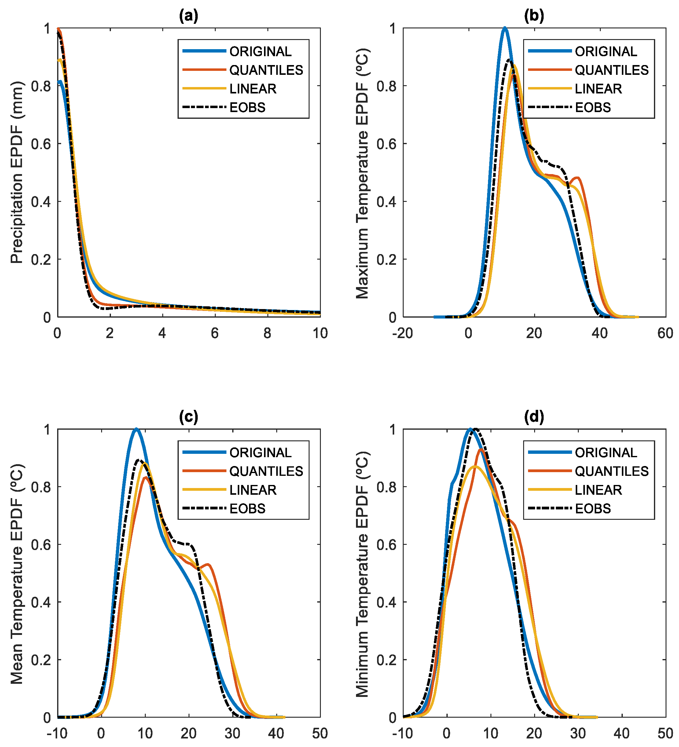
3.1. Comparison of Bias Correction Methods

In a first approach, the two bias correction methods were compared considering the variables: daily total precipitation (mm) and daily minimum, mean and maximum temperatures (°C). For a more detailed comparison, the transformed probability density functions, obtained after the application of each bias correction method, are compared. The kernel-density estimation of the EPDF (Figure 3) and the empirical cumulative distribution functions (ECDF; Figure S6) are represented for each variable, when pooling all grid boxes, considering the two bias correction methods, as well as the original (uncorrected) data and the E-OBS data (baseline for the correction). For the sake of succinctness, the simulations from the four model chains were pooled for estimating the EPDF. However, the corresponding plots for each model separately are shown as Supplementary Material (Figures S7–S10).

Precipitation is the variable with the least noticeable differences between the two correction methods (linear vs. quantiles, Figure 3a). Even so, it is possible to identify that both bias-corrected data present much more days with zero or near-zero precipitation than the original simulated data. This is a common result, as most climate models tend to underestimate the number of dry days [71]. Conversely, for daily precipitation > 1 mm (wet days), the bias-corrected data show lower probabilities than the original data. Moreover, these features are more accentuated for the quantile mapping method, which suggests that this method is more effective in correcting the above-referred underestimation of dry days by climate models.

The temperatures generally show a bimodal distribution, with a clear peak at lower temperatures (winter regime) and a secondary peak at higher temperatures (summer regime), which is a usual distribution in continental climate areas and is apparent in the E-OBS data. However, the simulated original data largely lack this bimodal structure, with a cool bias and an overestimation of the winter regime probability. This means that after bias correction, temperatures are shifted to the right in both bias-correction methods. For the future climates (2051–2080, RCP8.5), the linear method tends to depict a much smoother curve, where the peaks are less accentuated than in the quantile method, thus being mostly a shift to the right in the temperature EPDF (uniform warming). On the contrary, the data corrected by the quantile method show more pronounced bi-modal distributions than that obtained from the linear method. This ability to accurately replicate the observed winter/summer regimes in the bias-corrected data is a clear advantage of the former method and may have critical implications in the assessment of local/regional thermal conditions, namely in temperature accumulations and extremes.

A comparison between the two methods will be undertaken based on the above-mentioned indices of temperature and precipitation extremes and viticultural suitability. However, as expected, the differences in the annual mean variables between the future period (2051–2080) and the historical period (1989–2005) obtained from both bias correction methods are nearly equal, as they correspond to central tendency metrics, generally less affected by biases. For both methods, under RCP8.5, the area-mean of the daily mean temperature increases from approximately 13.0 °C to 15.5 °C (+ 1.5 °C warming), whereas the area-mean of annual total precipitation decreases from roughly 668 mm to 576 mm (−14%), thus hinting at the warming and drying trends over the upcoming decades. For the area-means of the daily maximum (minimum) temperature, the increase is 2.7 °C (1.9 °C).

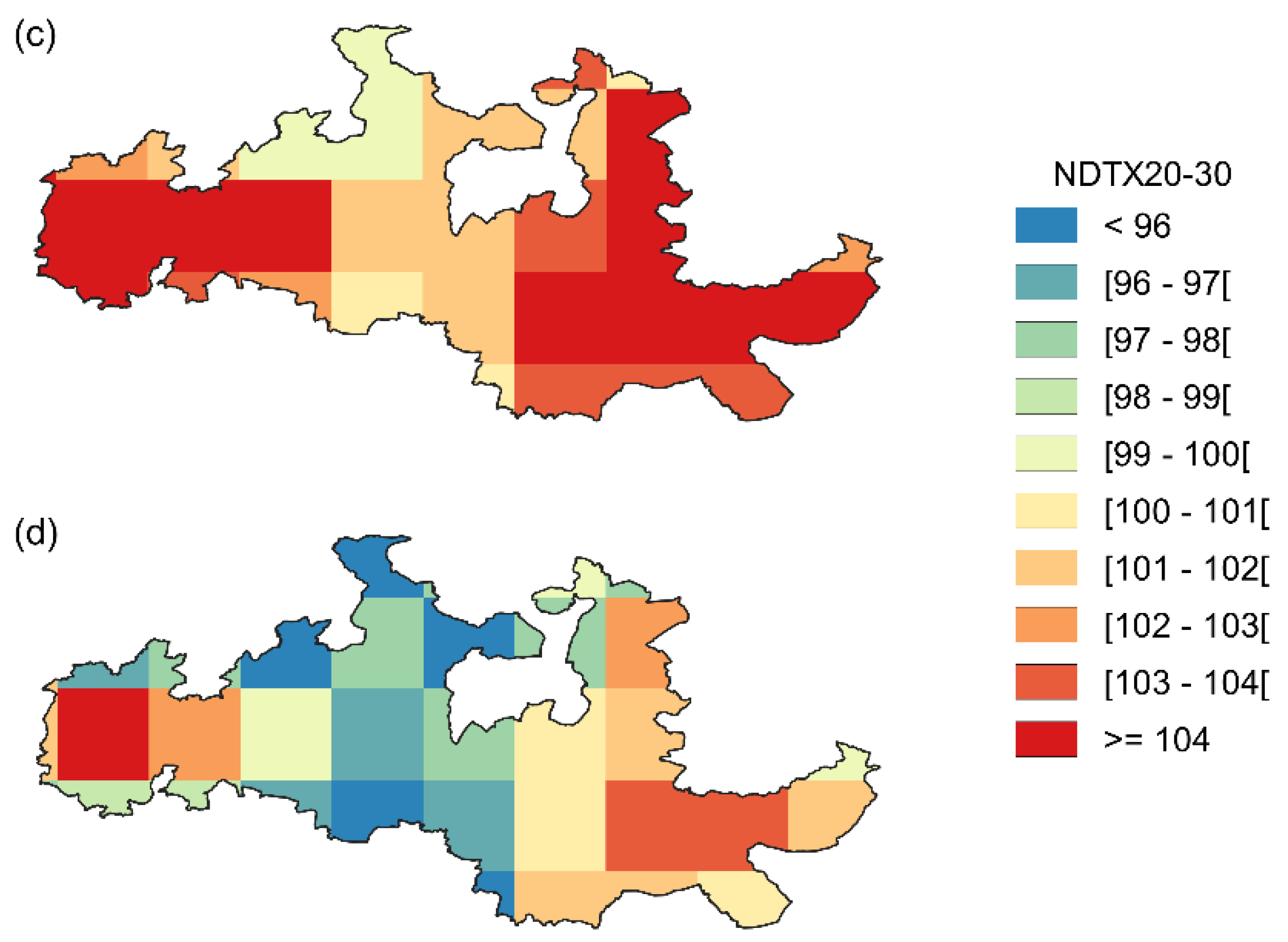
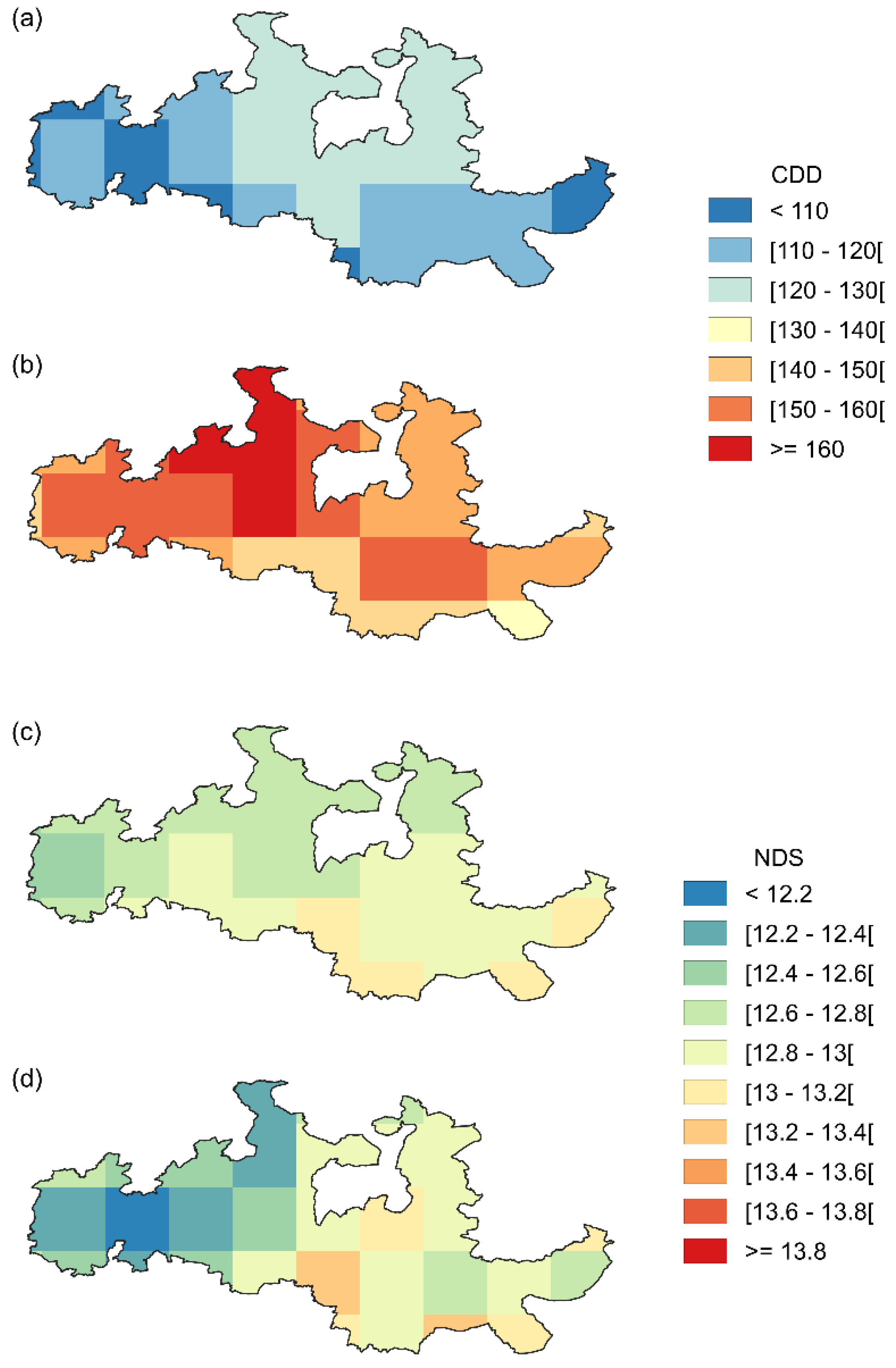
3.2. Indices: Linear vs. Quantile Corrections

The ensemble-mean patterns obtained from both bias correction methods over the future scenario will be compared to understanding the implications of the method’s choice in the indices and conclusions that can be drawn from them. To better evaluate the differences between both bias correction methods, the spatial root-mean-squared difference (RMSD) was calculated for the different climatic indices (

Table 1. Difference percentage between the linear and quantile mapping bias correction methods, using the root mean square error, for NDTX35 (Number of Days with maximum temperature, TX, above 35 °C), NDTX20-30 (Number of Days with maximum temperature, TX, between 20 and 30 °C), NWS (Number of Warm Spells), WSDI90 (Warm Spell Day Index above the 90th percentile), CDD (Consecutive Dry Days index), NDS (Number of Dry Spells), HI (Huglin Index), DI (Dryness Index), and GSP (Growing Season Precipitation). Statistically significant values at a confidence level of 99% are in bold.

NDTX35	NDTX20-30	NWS	WSDI90	CDD	NDS	HI	DI	GSP
13.4%	4.7%	12.3%	19.7%	19.5%	1.9%	3.3%	29.3%	22.7%

). The values were then normalized by the corresponding area-means (nRMSD) to allow their direct comparison. The nRMSD is computed as the mean of the squared grid box differences between two spatial patterns, which are herein the ensemble mean patterns for a given combination of an index, period, and bias-correction method. Hence, the nRMSD is a measure of the sensitivity of a given index to the choice of the bias correction method, i.e., a high value corresponds to high sensitivity.

For NDTX35 (Figure 4a,b), an index that reflects the prevalence of excessively warm conditions for temperate viticulture, the full range of values within the DWR is clearly larger using quantile mapping than the linear method, with much lower values in the higher-elevation areas of the westernmost part of the DWR and significantly higher frequencies of occurrence of extremely high temperatures in the upper Douro valley (eastern DWR). This finding is in agreement with the EPDF for maximum temperature, which shows that for temperatures superior to 35 °C, the quantile mapping method shows higher probabilities when compared to the linear method. Overall, the linear method shows lower values for the frequencies of occurrence of extremely high temperatures (about 5 days per year), particularly in the areas with higher exposure to climate change (Douro Superior, upper Douro valley), despite the high similarity between both spatial patterns. The nRMSD between both mean patterns is 13.4% (Table 1), which is a statistically significant value at a confidence level of 99%. Therefore, NDTX35 hints at the importance of having an adequate bias correction method when envisioning an analysis of extreme events and their corresponding impacts on, e.g., viticulture. Extreme indices are, by definition, concentrated on the tails of the EPDF, and slight differences in bias correction are thereby exacerbated, leading to inaccurate climate change impact assessments.

Regarding NDTX20-30 (Figure 4c,d), which corresponds to near-optimum maximum temperatures for grapevine development, the difference between the two bias correction methods is noteworthy, with the quantile mapping method showing slightly lower values when compared to the linear method. Thus, the linear method overestimates the frequencies of occurrence of days within this favorable temperature range, which is in accordance with the previously referred underestimation of extremely high temperatures. However, both methods display quite similar patterns, where the central area (Cima-Corgo) shows lower values with respect to the eastern and western parts. This finding is also attested by the minor nRMSD (4.7%), not statistically significant. Being an index more focused on central temperatures, the lower sensitivity to the bias correction can be anticipated.

For the case of the NWS (Figure 5a,b), the differences between the two correction methods reveal that the quantile method points to a slightly greater occurrence of warm spells, which is coherent with the previous findings for NDTX35. These warm episodes should occur between seven to eight times a year in the future climate, but there is a significant spatial difference between both methods (nRMSD of 12.3%, Table 1), with generally higher occurrences in the eastern region. Concerning the WSDI90 (Figure 5c,d), the quantile mapping method points again to a greater occurrence of warmer days and larger spatial gradients over the region, as expected, since this index is a direct manifestation of extremely high-temperature days. The nRMSD of 19.7% corroborates the significant differences between the two patterns.

The CDD (Figure 6a,b) index highlights the occurrence of extremely long dry periods and presents noteworthy differences between both bias correction methods (nRMSD of 19.5%). Once again, the quantile mapping presents higher values than the linear method, hinting at its ability to capture the dry periods. As previously stated, climate models often tend to underestimate the occurrence of dry days. Although the linear method already corrects a significant part of this bias, the quantile mapping is more effective in this correction and leads to a substantially higher number of dry days (precipitation < 1 mm).

Bearing in mind the aggregated nature of the NDS index (Figure 6c,d), its mean spatial patterns are not significantly different between both methods (nRMSD of 1.9%). However, it should be noted that the quantile method presents slightly greater contrasts between regions, which is a manifestation of the enhanced representation of dry days.

The indices of viticultural suitability are cumulative indices over the entire growing season (6-month period) and may, therefore, either offset or magnify the discrepancies between the bias correction methodologies on the daily timescale, depending on the exact location and strength of the biases in the EPDF. To our knowledge, no previous study has carried out such an assessment for these indices and the results should heavily depend on the index and location. As these indices have already been largely discussed for the DWR in previous studies [54,57,72,73], their maps are presented as supplementary material to avoid redundancy. However, the corresponding differences in terms of the bias correction methods are also documented here, owing to their essential role in viticultural zoning and climate change impact evaluation.

Regarding the HI (Supplementary Figure S11a,b), the linear method presents lower values than the quantile method in the most inland area (Douro Superior) and some parts of the western area, close to the Douro River. Nevertheless, the bias correction methods have little implications in the final pattern (nRMSD of 3.3%), thus suggesting a robust pattern. Conversely, the DI (Supplementary Figure S11c,d) shows significant differences between the two methods (nRMSD of 29.3%), with the innermost region typically experiencing lower values (higher dryness levels). For the case of GSP (Supplementary Figure S11e,f), it should be noted that the quantile method also presents greater spatial contrasts (nRMSD of 22.7%), revealing, e.g., maximum values in the southern-central border of the region, where mountain ranges are located and more intense and frequent convective precipitation is projected in the future (not shown). A similar feature is also found in DI (Figure S11d). In summary, while for HI only minor differences are found, for DI and GSP, the differences are noteworthy, highlighting the relevance of an adequate bias correction to safeguard their accurate estimation. The DI, in particular, is based on temperature–precipitation products, thus tending to present a non-linear response to input errors. This explains the highest sensitivity of this index to bias correction.

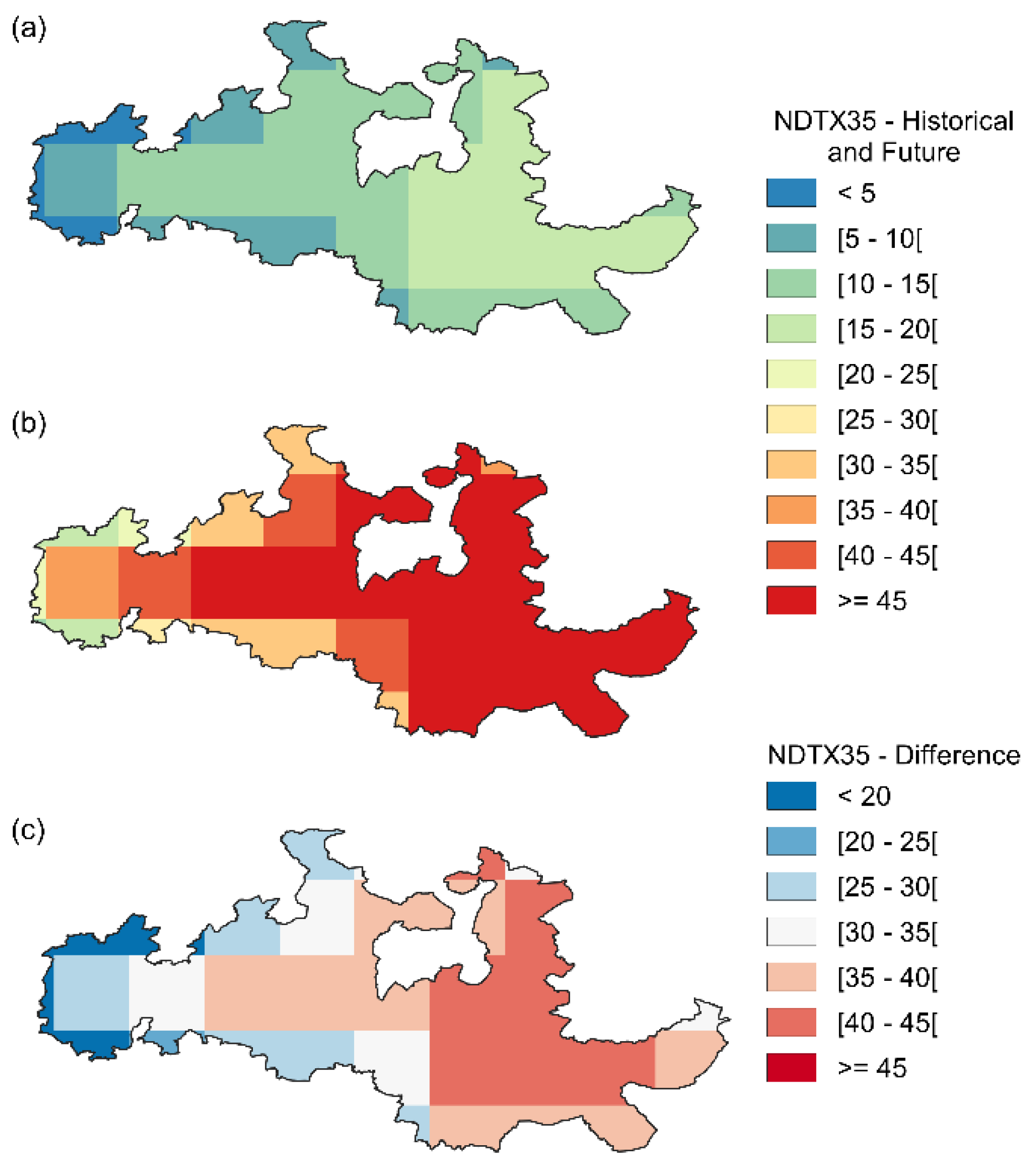
3.3. Climate Change Assessments

The previous section hints at the importance of an appropriate selection of a bias correction method to estimate the selected indices. This section considers the ensemble-mean patterns of the different indices over the historical and future periods, as well as their corresponding differences (climate change signal), using the quantile mapping method.

The NDTX35 (Figure 7) shows a considerable change between the two periods, evidencing a strong increase in the number of extremely warm days for the future period (from 20 to 45 days). The difference between periods is particularly pronounced in the eastern DWR (Douro Superior), a region that is already today significantly more exposed to these extremes. For the NDTX20-30 (Figure 8), a decrease in the number of days within this temperature range is apparent in the future, mostly in the western half of the DWR. This is a clear result of the sharp increase in the number of days with extremely high temperatures. The climate change signals of NDTX35 and NDTX20-30 are indeed complementary.

Due to the formulation of the NWS index (Figure 9), significant spatial differences are not evident. Nonetheless, a strong increase in the number of warm spells in the future period is projected, with a stronger signal in the northeastern region. These events are of less than one per year currently and are expected to reach, on average, eight occurrences per year in the future climate. This is a remarkable finding, as heatwaves were already reported to be potentially damaging for grapevines, mainly when heat stress is reinforced by water stress and high radiation levels [29]. Concomitantly, the WSDI90 (Figure 10) is one of the indices that shows a higher difference between the two periods, evidencing a notable warming trend. The increase ranges from 75 to 87 days per year, being also more noticeable in the northeastern region, in agreement with the changes for the NWS.

For the future period, an increase in the CDD index is also expected (Figure 11), which will be particularly apparent in the westernmost part of the DWR (>65 days), which is currently less exposed to droughts. The eastern region is already today quite dry, which explains the lower increases in CDD. On the other hand, for the NDS index (Figure 12), its values almost double throughout the DWR, mainly in the more continental (inner) region, i.e., the climate change projections indicate a shift from 7 to 8 spells to 12–14 spells per year, on average. Since these dry spells are key precursors of severe/extreme soil water deficits and water stress, more frequent droughts should be expected throughout the DWR in the future, with the above-mentioned implications for the regional viticulture.

For the HI (Figure S12), an overall increase in its values is evident in the future period, mostly in the central region (Cima-Corgo). Regarding the DI (Figure S13), a downward (drying) trend is projected, especially in the westernmost (Baixo-Corgo) and innermost (Douro Superior) areas. Similar considerations can be drawn regarding the GSP (Figure S14). Over the central area of the DWR (Cima-Corgo), the drying trends are, however, less prominent. A slight increase in GSP is, indeed, observed over the central-southern border of the DWR. This behavior is consistent with the increase in the frequencies of occurrence of extreme precipitation in this region projected by some climate models (not shown), which may imply additional risks in terms of heavy rainfall events, in many instances associated with deep convection, thunderstorms, and hailfall [74]. These meteorological hazards may also represent an increased risk for the region, but their assessment is out of the scope of the present study.

4. Discussion

Reliable information about how climate change over the forthcoming decades will impact crop development, growth, yield, and quality is essential for farmers and decision-makers. It promotes optimization of cultivation practices and management, reducing waste and economic losses, as well as potentiating a more efficient use of available resources, warranting environmental and socio-economic sustainability. More specifically, the present study findings provide evidence for multifaceted climate change impacts on the DWR viticulture, which is in agreement with previous studies [51,52,53,54]. Although GCM simulations are the most important tool to project these impacts, they neither provide regional-scale nor unbiased information [75]. Additionally, climate models are not able to represent with accuracy regional/local scale extreme events [76]. RCMs significantly contribute to overcoming these limitations, but important biases are still reminiscent in their simulations. For this reason, it is important to apply appropriate bias correction methods to model outputs to avoid considerably hampering the accuracy of future projections. Several studies have been comparing different bias correction methods to assess their performance under different conditions, regions, and variables [39,41,77,78]. In the study of [78], seven bias correction methods were tested for precipitation and five for temperature. The results show that the quantile mapping methods are by far the best-performing for precipitation projections. This conclusion was also verified in the study of [77].

The present study results reveal that the selection of different bias correction methods can significantly impact the conclusions. Regarding the two methods studied here, the linear method is the simplest and least computationally demanding. Furthermore, the differences between this method and the quantile mapping are not always noteworthy. However, the results regarding extreme events revealed remarkable differences. For the NDTX35, NWS, WSDI90, and CDD indices, the linear method visibly shows lower values than the quantile mapping method. This occurs because the linear methods apply the same correction over the whole data series, regardless of being central or extreme values. Overall, the mathematical definition of each index underlies its higher/lower sensitivity. Indices with non-linear formulations and/or based on tail distributions are commonly more prone to error propagation and magnification. Considering the aforementioned limitations of the climate models in realistically replicating extreme events (defined on the tails of the distributions), this is a clear shortcoming of the linear approach.

The air temperature is considered one of the most important atmospheric variables considering the development and growth of the grapevines [43], as cool conditions [79] or extreme heat [80] can affect vine physiology and yield. During the growing season, the average air temperature should lie preferably between 12–13 °C and 22–24 °C. Lower temperatures cannot promote the proper development of the grapevine, while higher temperatures combined with low precipitation can trigger heat stress. On the other hand, high temperatures, combined with high precipitation, may trigger pests and diseases [26]. The results show that extreme temperatures (NDTX35, NWS, and WSDI90) will tend to be more severe in a future climate. For the case of NDTX35, an increase of almost 400% is verified. Regarding the number of warm spells, 7 events/year are expected, with a minimum duration of 6 days, meaning that at least 42 days/year will be under heatwave conditions. The WSDI90 also presents relevant values, since the number of days will approximately increase from 75 to 90. Heatwaves during the veraison-maturity period can significantly influence sugar accumulation [81]. Moreover, high temperatures can strongly impact the sensory character of wines [82]. Regarding the NDTX20-30, the projected decrease is noticeable under the future scenario. This is an indirect result of the increase in the number of days with extremely high temperatures. Therefore, the susceptibility of the DWR to extremely high temperatures is projected to increase very significantly in the forthcoming decades, which will represent a noteworthy threat to the regional winemaking sector.

Precipitation is responsible for determining soil water availability and, for that reason, it is also a critical atmospheric variable for grapevine development [26]. Recent studies show that water deficits can affect grape berry attributes, wine typicity, and profile [83,84]. During budburst and shoot/inflorescence development, water stress can cause small shoot growth, poor flower clusters, and berry set development [85]. However, during the development stage of the grapevine, moderately dry soils might be favorable to the production of high-quality wines [86]. The DI is based on the potential water available in the soil and is also related to grapevine growth, yield, and wine quality [68]. It encompasses four classes, varying from very dry (DI ≤ 100 mm) to humid (DI > 150 mm) conditions. The Thornthwaite method is used for estimating the potential evapotranspiration (PET) in DI [48]. Although the PET estimation can be significantly under- or overestimated under future climate conditions, with implications in the DI values, the present study is mainly focused on the comparison of the potential impacts of bias-correction methods. Thus, an invariant definition of DI, exclusively reflecting changes in the input variables (temperatures and precipitation), should thereby be considered for both the historical and future periods. The results of this index show a strengthening of dryness, as the values decrease nearly 60 mm throughout the DWR. Still, for both historical and future periods, the classification remains the same: moderately dry (−100 ≤ DI > −50). The precipitation during the favorable period also decreases, except for a small mountainous area in the southern-central border, which should undergo a slight increase. Regarding the extreme climate events, the number of dry spells is projected to increase from approx. 7.5 to approx. 13 per year, which is a near doubling of events. Furthermore, the CDD will increase in the majority of the study region. This drying trend has been identified in several previous studies and for many southern European regions, e.g., southern Spain, Portugal, or Italy [87]. As a result, the implementation and installation of smart deficit irrigation systems have been advocated as one possible adaptation strategy to maintain wine production and quality of some winemaking regions [88].

5. Conclusions

Viticulture is strongly dependent on weather and climatic conditions, thus being largely exposed and vulnerable to changing climates. The present study hints at the critical importance of using adequate bias-correction methods for the treatment of RCM output data. Different bias correction methods may imply different results, especially concerning extreme weather events. For that reason, the future projections developed herein were corrected using quantile mapping. For the DWR, some viticulture-relevant climatic changes are documented, namely the drying and warming trends, but also a notorious increase in the number of extreme events (extremely warm days, heatwaves, long-lasting dry spells, and droughts). These changes may have detrimental impacts on viticulture and wine quality, emphasizing the importance of this study and the importance of outlining suitable adaptation strategies for reducing climate change impacts and risks.

References

1. IPCC. Climate Change 2014: Synthesis Report, Contribution of Working Groups I, II and III to the Fifth Assessment Report of the Intergovernmental Panel on Climate Change; IPCC: Geneva, Switzerland, 2014; Volume 218, ISBN 9789291691432. [Google Scholar]
2. Frich, P.; Alexander, L.V.; Della-Marta, P.; Gleason, B.; Haylock, M.; Tank Klein, A.M.G.; Peterson, T. Observed coherent changes in climatic extremes during the second half of the twentieth century. Clim. Res. 2002, 19, 193–212. [Google Scholar] [CrossRef] [Green Version]
3. Klein Tank, A.M.G.; Wijngaard, J.B.; Können, G.P.; Böhm, R.; Demarée, G.; Gocheva, A.; Mileta, M.; Pashiardis, S.; Hejkrlik, L.; Kern-Hansen, C.; et al. Daily dataset of 20th-century surface air temperature and precipitation series for the European Climate Assessment. Int. J. Climatol. 2002, 22, 1441–1453. [Google Scholar] [CrossRef]
4. Alexander, L.V.; Zhang, X.; Peterson, T.C.; Caesar, J.; Gleason, B.; Klein Tank, A.M.G.; Haylock, M.; Collins, D.; Trewin, B.; Rahimzadeh, F.; et al. Global observed changes in daily climate extremes of temperature and precipitation. J. Geophys. Res. Atmos. 2006, 111, 1–22. [Google Scholar] [CrossRef] [Green Version]
5. Della-Marta, P.M.; Haylock, M.R.; Luterbacher, J.; Wanner, H. Doubled length of western European summer heat waves since 1880. J. Geophys. Res. Atmos. 2007, 112, 1–11. [Google Scholar] [CrossRef] [Green Version]
6. Moberg, A.; Jones, P.D.; Lister, D.; Walther, A.; Brunet, M.; Jacobeit, J.; Alexander, L.V.; Della-Marta, P.M.; Luterbacher, J.; Yiou, P.; et al. Indices for daily temperature and precipitation extremes in Europe analyzed for the period 1901–2000. J. Geophys. Res. Atmos. 2006, 111. [Google Scholar] [CrossRef] [Green Version]
7. Peings, Y.; Cattiaux, J.; Douville, H. Evaluation and response of winter cold spells over Western Europe in CMIP5 models. Clim. Dyn. 2013, 41, 3025–3037. [Google Scholar] [CrossRef]
8. Russo, S.; Sillmann, J.; Fischer, E.M. Top ten European heatwaves since 1950 and their occurrence in the coming decades. Environ. Res. Lett. 2015, 10. [Google Scholar] [CrossRef]
9. Cardoso, R.M.; Soares, P.M.M.; Lima, D.C.A.; Miranda, P.M.A. Mean and extreme temperatures in a warming climate: EURO CORDEX and WRF regional climate high-resolution projections for Portugal. Clim. Dyn. 2019, 52, 129–157. [Google Scholar] [CrossRef]
10. Sillmann, J.; Kharin, V.V.; Zwiers, F.W.; Zhang, X.; Bronaugh, D. Climate extremes indices in the CMIP5 multimodel ensemble: Part 2. Future climate projections. J. Geophys. Res. Atmos. 2013, 118, 2473–2493. [Google Scholar] [CrossRef]
11. Karagiannidis, A.F.; Karacostas, T.; Maheras, P.; Makrogiannis, T. Climatological aspects of extreme precipitation in Europe, related to mid-latitude cyclonic systems. Theor. Appl. Climatol. 2012, 107, 165–174. [Google Scholar] [CrossRef]
12. Costa, A.C.; Soares, A. Trends in extreme precipitation indices derived from a daily rainfall database for the South of Portugal. Int. J. Climatol. 2009, 29, 1956–1975. [Google Scholar] [CrossRef]
13. De Lima, M.I.P.; Santo, F.E.; Ramos, A.M.; Trigo, R.M. Trends and correlations in annual extreme precipitation indices for mainland Portugal, 1941–2007. Theor. Appl. Climatol. 2015, 119, 55–75. [Google Scholar] [CrossRef]
14. Rajczak, J.; Schär, C. Projections of Future Precipitation Extremes Over Europe: A Multimodel Assessment of Climate Simulations. J. Geophys. Res. Atmos. 2017, 122, 10–773. [Google Scholar] [CrossRef]
15. de Melo-Gonçalves, P.; Rocha, A.; Santos, J.A. Robust inferences on climate change patterns of precipitation extremes in the Iberian Peninsula. Phys. Chem. Earth 2016, 94, 114–126. [Google Scholar] [CrossRef]
16. Santos, M.; Fonseca, A.; Fragoso, M.; Santos, J.A. Recent and future changes of precipitation extremes in mainland Portugal. Theor. Appl. Climatol. 2019, 137, 1305–1319. [Google Scholar] [CrossRef]
17. Costa, A.C.; Santos, J.A.; Pinto, J.G. Climate change scenarios for precipitation extremes in Portugal. Theor. Appl. Climatol. 2012, 217–234. [Google Scholar] [CrossRef]
18. Cardoso Pereira, S.; Marta-Almeida, M.; Carvalho, A.C.; Rocha, A. Extreme Precipitation Events under Climate Change in the Iberian Peninsula. Int. J. Climatol. 2018, 40, 1255–1278. [Google Scholar] [CrossRef]
19. Santos, J.A.; Pinto, J.G.; Ulbrich, U. On the development of strong ridge episodes over the eastern North Atlantic. Geophys. Res. Lett. 2009, 36, L17804. [Google Scholar] [CrossRef] [Green Version]
20. Viceto, C.; Pereira, S.C.; Rocha, A. Climate change projections of extreme temperatures for the Iberian Peninsula. Atmosphere 2019, 10, 229. [Google Scholar] [CrossRef] [Green Version]
21. Serrano, J.P.; Díaz, F.J.A.; García, J.A.G. Analysis of extreme temperature events over the Iberian Peninsula during the 21st century using dynamic climate projections chosen using max-stable processes. Atmosphere 2020, 11, 506. [Google Scholar] [CrossRef]
22. Drobinski, P.; Da Silva, N.; Bastin, S.; Mailler, S.; Muller, C.; Ahrens, B.; Christensen, O.B.; Lionello, P. How warmer and drier will the Mediterranean region be at the end of the twenty-first century? Reg. Environ. Chang. 2020, 20. [Google Scholar] [CrossRef]
23. Yu, H.; Wu, D.; Piao, X.; Zhang, T.; Yan, Y.; Tian, Y.; Li, Q.; Cui, X. Reduced impacts of heat extremes from limiting global warming to under 1.5 °C or 2 °C over Mediterranean regions. Environ. Res. Lett. 2021, 16. [Google Scholar] [CrossRef]
24. Fraga, H.; Pinto, J.G.; Viola, F.; Santos, J.A. Climate change projections for olive yields in the Mediterranean Basin. Int. J. Climatol. 2020, 40, 769–781. [Google Scholar] [CrossRef] [Green Version]
25. Van Leeuwen, C.; Friant, P.; Choné, X.; Tregoat, O.; Koundouras, S.; Dubourdieu, D. Influence of climate, soil, and cultivar on terroir. Am. J. Enol. Vitic. 2004, 55, 207–217. [Google Scholar]
26. Santos, J.A.; Fraga, H.; Malheiro, A.C.; Moutinho-Pereira, J.; Dinis, L.T.; Correia, C.; Moriondo, M.; Leolini, L.; Dibari, C.; Costafreda-Aumedes, S.; et al. A review of the potential climate change impacts and adaptation options for European viticulture. Appl. Sci. 2020, 10, 3092. [Google Scholar] [CrossRef]
27. Parker, A.K.; De Cortázar-Atauri, I.G.; Van Leeuwen, C.; Chuine, I. General phenological model to characterise the timing of flowering and veraison of Vitis vinifera L. Aust. J. Grape Wine Res. 2011, 17, 206–216. [Google Scholar] [CrossRef]
28. Lereboullet, A.L.; Beltrando, G.; Bardsley, D.K.; Rouvellac, E. The viticultural system and climate change: Coping with long-term trends in temperature and rainfall in Roussillon, France. Reg. Environ. Chang. 2014, 14, 1951–1966. [Google Scholar] [CrossRef]
29. Fraga, H.; Molitor, D.; Leolini, L.; Santos, J.A. What Is the Impact of Heatwaves on European Viticulture? A Modelling Assessment. Appl. Sci. 2020, 10, 3030. [Google Scholar] [CrossRef]
30. Van Leeuwen, C.; Tregoat, O.; Choné, X.; Bois, B.; Pernet, D.; Gaudillére, J.P. Vine water status is a key factor in grape ripening and vintage quality for red bordeaux wine. How can it be assessed for vineyard management purposes? J. Int. Sci. Vigne Vin 2009, 43, 121–134. [Google Scholar] [CrossRef]
31. Ollé, D.; Guiraud, J.L.; Souquet, J.M.; Terrire, N.; Ageorges, A.; Cheynier, V.; Verries, C. Effect of pre- and post-veraison water deficit on proanthocyanidin and anthocyanin accumulation during Shiraz berry development. Aust. J. Grape Wine Res. 2011, 17, 90–100. [Google Scholar] [CrossRef]
32. Le Menn, N.; Van Leeuwen, C.; Picard, M.; Riquier, L.; De Revel, G.; Marchand, S. Effect of Vine Water and Nitrogen Status, as Well as Temperature, on Some Aroma Compounds of Aged Red Bordeaux Wines. J. Agric. Food Chem. 2019. [Google Scholar] [CrossRef] [PubMed]
33. Picard, M.; van Leeuwen, C.; Guyon, F.; Gaillard, L.; de Revel, G.; Marchand, S. Vine Water Deficit Impacts Aging Bouquet in Fine Red Bordeaux Wine. Front. Chem. 2017, 5, 56. [Google Scholar] [CrossRef] [PubMed] [Green Version]
34. Guilpart, N.; Metay, A.; Gary, C. Grapevine bud fertility and number of berries per bunch are determined by water and nitrogen stress around flowering in the previous year. Eur. J. Agron. 2014, 54, 9–20. [Google Scholar] [CrossRef]
35. Huglin, M.P. Nouveau mode d’évaluation des possibilités héliothermiques d’un milieu viticole. Comptes Rendus Académie Agric. Fr. 1978, 64, 1117–1126. [Google Scholar]
36. Solomon, S.; Qin, D.; Manning, M.; Chen, Z.; Marquis, M.; Averyt, K.B.; Tignor, M.; Miller, H.L.; IPCC (Eds.) Climate Change 2007: The Physical Science Basis. Contribution of Working Group I to the Fourth Assessment Report of the Intergovernmental Panel on Climate Change; Cambridge University Press: Cambridge, UK; New York, NY, USA, 2007. [Google Scholar]
37. Casanueva, A.; Kotlarski, S.; Herrera, S.; Fernández, J.; Gutiérrez, J.M.; Boberg, F.; Colette, A.; Christensen, O.B.; Goergen, K.; Jacob, D.; et al. Daily precipitation statistics in a EURO-CORDEX RCM ensemble: Added value of raw and bias-corrected high-resolution simulations. Clim. Dyn. 2016, 47, 719–737. [Google Scholar] [CrossRef] [Green Version]
38. Velasquez, P.; Messmer, M.; Raible, C.C. A new bias-correction method for precipitation over complex terrain suitable for different climate states: A case study using WRF ( version 3. 8. 1). Geosci. Model Dev. 2020, 13, 5007–5027. [Google Scholar] [CrossRef]
39. Ishizaki, N.N.; Nishimori, M.; Iizumi, T.; Shiogama, H. Evaluation of Two Bias-Correction Methods for Gridded Climate Scenarios over Japan. SOLA 2020, 16, 80–85. [Google Scholar] [CrossRef] [Green Version]
40. Singh, D.; Mohite, A.R.; Pratyasha, P.; Khatun, A. Impact of climate change on streamflow regime of a large Indian river basin using a novel monthly hybrid bias correction technique and a conceptual modeling framework. J. Hydrol. 2020, 590, 125448. [Google Scholar] [CrossRef]
41. François, B.; Vrac, M.; Cannon, A.J.; Robin, Y.; Allard, D.; Cnrs, E.L.; Uvsq, C.E.A. Multivariate bias corrections of climate simulations: Which benefits for which losses? Earth Syst. Dyn. 2020, 11, 537–562. [Google Scholar] [CrossRef]
42. Passow, C. Regression-based distribution mapping for bias correction of climate model outputs using linear quantile regression. Stoch. Environ. Res. Risk Assess. 2020, 34, 87–102. [Google Scholar] [CrossRef]
43. Fraga, H.; Pinto, J.; Santos, J. Climate change projections for chilling and heat forcing conditions in European vineyards and olive orchards: A multi-model assessment. Clim. Chang. 2019, 152, 179–193. [Google Scholar] [CrossRef]
44. Wang, Z.; Wen, X.; Lei, X.; Tan, Q.; Fang, G.; Zhang, X. Effects of different statistical distribution and threshold criteria in extreme precipitation modelling over global land areas. Int. J. Climatol. 2020, 40, 1838–1850. [Google Scholar] [CrossRef]
45. Chen, W.; Zhu, D.; Ciais, P.; Huang, C.; Viovy, N.; Kageyama, M. Response of vegetation cover to CO2 and climate changes between Last Glacial Maximum and pre-industrial period in a dynamic global vegetation model. Quat. Sci. Rev. 2019, 218, 293–305. [Google Scholar] [CrossRef]
46. Zhao, Y.; Liu, Y.L.; Guo, Z.T.; Fang, K.Y.; Li, Q.; Cao, X.Y. Abrupt vegetation shifts caused by gradual climate changes in central Asia during the Holocene. Sci. China Earth Sci. 2017, 60, 1317–1327. [Google Scholar] [CrossRef]
47. Maraun, D. Bias Correcting Climate Change Simulations–A Critical Review. Curr. Clim. Chang. Rep. 2016, 2, 211–220. [Google Scholar] [CrossRef] [Green Version]
48. Fraga, H.; García de Cortázar Atauri, I.; Malheiro, A.C.; Moutinho-Pereira, J.; Santos, J.A. Viticulture in Portugal: A review of recent trends and climate change projections. Oeno One 2017, 51, 61–69. [Google Scholar] [CrossRef] [Green Version]
49. Real, A.C.; Borges, J.; Cabral, J.S.; Jones, G.V. Partitioning the grapevine growing season in the Douro Valley of Portugal: Accumulated heat better than calendar dates. Int. J. Biometeorol. 2015, 59, 1045–1059. [Google Scholar] [CrossRef]
50. Santos, J.A.; Ceglar, A.; Toreti, A.; Prodhomme, C. Performance of seasonal forecasts of Douro and Port wine production. Agric. For. Meteorol. 2020, 291, 108095. [Google Scholar] [CrossRef]
51. Fraga, H.; Santos, J.A.; Malheiro, A.C.; Oliveira, A.A.; Moutinho-Pereira, J.; Jones, G.V. Climatic suitability of Portuguese grapevine varieties and climate change adaptation. Int. J. Climatol. 2016, 36, 1–12. [Google Scholar] [CrossRef]
52. Santos, J.A.; Grätsch, S.D.; Karremann, M.K.; Jones, G.V.; Pinto, J.G. Ensemble projections for wine production in the Douro Valley of Portugal. Clim. Chang. 2013, 117, 211–225. [Google Scholar] [CrossRef]
53. Santos, J.A.; Malheiro, A.C.; Karremann, M.K.; Pinto, J.G. Statistical modelling of grapevine yield in the Port Wine region under present and future climate conditions. Int. J. Biometeorol. 2011, 55, 119–131. [Google Scholar] [CrossRef] [PubMed]
54. Santos, M.; Fonseca, A.; Fraga, H.; Jones, G.V.; Santos, J.A. Bioclimatic conditions of the Portuguese wine denominations of origin under changing climates. Int. J. Climatol. 2019, 1–15. [Google Scholar] [CrossRef]
55. Fonseca, A.R.; Santos, J.A. High-resolution temperature datasets in Portugal from a geostatistical approach: Variability and extremes. J. Appl. Meteorol. Climatol. 2018, 57, 627–644. [Google Scholar] [CrossRef]
56. Fraga, H.; Santos, J.A. Daily prediction of seasonal grapevine production in the Douro wine region based on favourable meteorological conditions. Aust. J. Grape Wine Res. 2017, 23, 296–304. [Google Scholar] [CrossRef]
57. Blanco-Ward, D.; Monteiro, A.; Lopes, M.; Borrego, C.; Silveira, C.; Viceto, C.; Rocha, A.; Ribeiro, A.; Andrade, J.; Feliciano, M.; et al. Climate change impact on a wine-producing region using a dynamical downscaling approach: Climate parameters, bioclimatic indices and extreme indices. Int. J. Climatol. 2019, 39, 5741–5760. [Google Scholar] [CrossRef]
58. Fraga, H.; Malheiro, A.C.; Moutinho-Pereira, J.; Cardoso, R.M.; Soares, P.M.M.; Cancela, J.J.; Pinto, J.G.; Santos, J.A. Integrated analysis of climate, soil, topography and vegetative growth in iberian viticultural regions. PLoS ONE 2014, 9. [Google Scholar] [CrossRef]
59. Fraga, H.; Costa, R.; Santos, J.A. Multivariate clustering of viticultural terroirs in the Douro winemaking region. Cienc. Tec. Vitivinic. 2017, 32, 142–153. [Google Scholar] [CrossRef] [Green Version]
60. Cornes, R.C.; van der Schrier, G.; van den Besselaar, E.J.M.; Jones, P.D. An Ensemble Version of the E-OBS Temperature and Precipitation Data Sets. J. Geophys. Res. Atmos. 2018, 123, 9391–9409. [Google Scholar] [CrossRef] [Green Version]
61. Klein Tank, A.M.G.; Können, G.P. Trends in Indices of daily temperature and precipitation extremes in Europe, 1946–1999. J. Clim. 2003, 16, 3665–3680. [Google Scholar] [CrossRef]
62. Jacob, D.; Petersen, J.; Eggert, B.; Alias, A.; Christensen, O.B.; Bouwer, L.M.; Braun, A.; Colette, A.; Déqué, M.; Georgievski, G.; et al. EURO-CORDEX: New high-resolution climate change projections for European impact research. Reg. Environ. Chang. 2014, 14, 563–578. [Google Scholar] [CrossRef]
63. Christensen, J.H.; Kjellström, E.; Giorgi, F.; Lenderink, G.; Rummukainen, M. Weight assignment in regional climate models. Clim. Res. 2010, 44, 179–194. [Google Scholar] [CrossRef]
64. Jacob, D.; Teichmann, C.; Sobolowski, S.; Katragkou, E.; Anders, I.; Belda, M.; Benestad, R.; Boberg, F.; Buonomo, E.; Cardoso, R.M.; et al. Regional climate downscaling over Europe: Perspectives from the EURO-CORDEX community. Reg. Environ. Chang. 2020, 20. [Google Scholar] [CrossRef]
65. Peterson, T.C.; Folland, C.; Gruza, G.; Hogg, W.; Mokssit, A.; Plummer, N. Report on the Activities of the Working Group on Climate Change Detection and Related Rapporteurs; Report on the Activities of the Working Group on Climate Change Detection and Related Rapporteurs Methods with emphasis on analyses of extreme events; World Meteorological Organization: Geneva, Switzerland, 2001; p. 144. [Google Scholar]
66. Karl, T.R.; Nicholls, N.; Ghazi, A. Clivar/GCOS/WMO Workshop on Indices and Indicators for Climate Extremes Workshop Summary. Clim. Chang. 1999, 42, 3–7. [Google Scholar] [CrossRef]
67. Riou, C.; European Union. Le Déterminisme Climatique de la Maturation du Raisin: Application au Zonage de la Teneur en Sucre Dans la Communauté Européenne; Publications Office of the European Union: Luxembourg, 1994. [Google Scholar]
68. Hardie, W.J.; Martin, S.R. Shoot growth on de-fruited grapevines: A physiological indicator for irrigation scheduling. Aust. J. Grape Wine Res. 2000, 6, 52–58. [Google Scholar] [CrossRef]
69. Amengual, A.; Homar, V.; Romero, R.; Alonso, S.; Ramis, C. A statistical adjustment of regional climate model outputs to local scales: Application to Platja de Palma, Spain. J. Clim. 2012, 25, 939–957. [Google Scholar] [CrossRef] [Green Version]
70. Miao, C.; Su, L.; Sun, Q.; Duan, Q. A nonstationary bias-correction technique to remove bias in GCM simulations. J. Geophys. Res. Atmos. 2016, 121, 5718–5735. [Google Scholar] [CrossRef]
71. Fowler, H.J.; Ekström, M.; Blenkinsop, S.; Smith, A.P. Estimating change in extreme European precipitation using a multimodel ensemble. J. Geophys. Res. Atmos. 2007, 112. [Google Scholar] [CrossRef] [Green Version]
72. Malheiro, A.C.; Santos, J.A.; Fraga, H.; Pinto, J.G. Climate change scenarios applied to viticultural zoning in Europe. Clim. Res. 2010, 43, 163–177. [Google Scholar] [CrossRef] [Green Version]
73. Fraga, H.; Malheiro, A.C.; Moutinho-Pereira, J.; Jones, G.V.; Alves, F.; Pinto, J.G.; Santos, J.A. Very high resolution bioclimatic zoning of Portuguese wine regions: Present and future scenarios. Reg. Environ. Chang. 2014, 14, 295–306. [Google Scholar] [CrossRef]
74. Santos, J.A.; Belo-Pereira, M. A comprehensive analysis of hail events in Portugal: Climatology and consistency with atmospheric circulation. Int. J. Climatol. 2019, 39, 188–205. [Google Scholar] [CrossRef] [Green Version]
75. Collins, M.; Knutti, R.; Arblaster, J.; Dufresne, J.-L.; Fichefet, T.; Friedlingstein, P.; Gao, X.; Gutowski, W.J.; Johns, T.; Krinner, G.; et al. Long-term Climate Change: Projections, Commitments and Irreversibility. In Climate Change 2013-The Physical Science Basis: Contribution of Working Group I to the Fifth Assessment Report of the Intergovernmental Panel on Climate Change; Cambridge University Press: Cambridge, UK, 2013; pp. 1029–1136. [Google Scholar]
76. Volosciuk, C.; Maraun, D.; Semenov, V.A.; Park, W. Extreme precipitation in an atmosphere general circulation model: Impact of horizontal and vertical model resolutions. J. Clim. 2015, 28, 1184–1205. [Google Scholar] [CrossRef] [Green Version]
77. Soriano, E.; Mediero, L.; Garijo, C. Selection of Bias Correction Methods to Assess the Impact of Climate Change on Flood Frequency Curves. Water 2019, 11, 2266. [Google Scholar] [CrossRef] [Green Version]
78. Luo, M.; Liu, T.; Meng, F.; Duan, Y.; Frankl, A.; Bao, A.; Maeyer, P. De Comparing Bias Correction Methods Used in Downscaling Precipitation and Temperature from Regional Climate Models: A Case Study from the Kaidu River Basin in Western China. Water 2018, 10, 1046. [Google Scholar] [CrossRef] [Green Version]
79. Mosedale, J.R.; Wilson, R.J.; Maclean, I.M.D. Climate Change and Crop Exposure to Adverse Weather: Changes to Frost Risk and Grapevine Flowering Conditions. PLoS ONE 2015, 10, e0141218. [Google Scholar] [CrossRef] [PubMed] [Green Version]
80. Molitor, D.; Keller, M. Yield of Müller-Thurgau and Riesling grapevines is altered by meteorological conditions in the current and previous growing seasons. Oeno One 2016, 50, 245–258. [Google Scholar] [CrossRef] [Green Version]
81. Greer, D.H.; Weedon, M.M. The impact of high temperatures on Vitis vinifera cv. Semillon grapevine performance and berry ripening. Front. Plant Sci. 2013, 4, 491. [Google Scholar] [CrossRef] [PubMed] [Green Version]
82. Robinson, A.L.; Boss, P.K.; Solomon, P.S.; Trengove, R.D.; Heymann, H.; Ebeler, S.E. Origins of grape and wine aroma. Part 1. Chemical components and viticultural impacts. Am. J. Enol. Vitic. 2014, 65, 1–24. [Google Scholar] [CrossRef] [Green Version]
83. Savoi, S.; Wong, D.C.J.; Arapitsas, P.; Miculan, M.; Bucchetti, B.; Peterlunger, E.; Fait, A.; Mattivi, F.; Castellarin, S.D. Transcriptome and metabolite profiling reveals that prolonged drought modulates the phenylpropanoid and terpenoid pathway in white grapes (Vitis vinifera L.). BMC Plant Biol. 2016, 16, 67. [Google Scholar] [CrossRef] [Green Version]
84. Vilanova, M.; Fandiño, M.; Frutos-Puerto, S.; Cancela, J.J. Assessment fertigation effects on chemical composition of Vitis vinifera L. cv. Albariño. Food Chem. 2019, 278, 636–643. [Google Scholar] [CrossRef]
85. Hardie, W.J.; Considine, J.A. Response of Grapes to Water-Deficit Stress in Particular Stages of Development. Am. J. Enol. Vitic. 1976, 27, 55–61. [Google Scholar]
86. Ramos, M.C.; Jones, G.V.; Martínez-Casasnovas, J.A. Structure and trends in climate parameters affecting winegrape production in northeast Spain. Clim. Res. 2008, 38, 1–15. [Google Scholar] [CrossRef] [Green Version]
87. Kenny, G.J.; Harrison, P.A. The Effects of Climate Variability and Change on Grape Suitability in Europe. J. Wine Res. 1992, 3, 163–183. [Google Scholar] [CrossRef]
88. Fraga, H.; García de Cortázar Atauri, I.; Santos, J.A. Viticultural irrigation demands under climate change scenarios in Portugal. Agric. Water Manag. 2018, 196, 66–74. [Google Scholar] [CrossRef]
Figure 1. (a) Geographical location of the Douro Wine Region (DWR) in Europe and Portugal. (b) Hypsometric chart of the DWR (elevation in m). The coordinate system of the used projections is WGS 84.
Agronomy 11 00990 g001
Figure 2. Empirical probability distribution functions (EPDF), with kernel-density estimation, for the historical period (1989–2005), for the daily (a) total precipitation, (b) maximum temperature, (c) mean temperature, and (d) minimum temperature, for E-OBS data (dashed black line), bias-corrected data using the quantile mapping (orange line) and linear (yellow line) methods, and the original model simulation data (no bias correction for the historical period; purple line).
Agronomy 11 00990 g002
Figure 3. Empirical probability distribution functions (EPDF), with kernel-density estimation, for the future period (2051–2080) under the RCP8.5 scenario for the daily (a) total precipitation, (b) maximum temperature, (c) mean temperature, and (d) minimum temperature, for the original model simulation data (no bias correction; blue line) and the bias-corrected data using the quantile mapping (orange line) and linear (yellow line) methods. The corresponding EPDFs for E-OBS data are also depicted (historical data; dashed black line).
Agronomy 11 00990 g003
Figure 4. Ensemble-mean of the Number of Days with maximum temperatures above 35 °C (NDTX35) for the Douro Wine Region and the future period (2051–2080), under the RCP8.5, with a bias correction following the (a) linear and (b) quantile mapping methods. (c,d) The same as (a,b) but for the Number of Days with maximum temperatures between 20 and 30 °C (NDTX20-30).
Agronomy 11 00990 g004aAgronomy 11 00990 g004b
Figure 5. Ensemble-mean of the Number of Warm Spells (NWS) for the Douro Wine Region and the future period (2051–2080), under the RCP8.5, with a bias correction following the (a) linear and (b) quantile mapping methods. (c,d) The same as (a,b) but for the Warm Spell Day Index above the 90th percentile (WSDI90).
Agronomy 11 00990 g005
Figure 6. Ensemble-mean of the Consecutive Dry Days index (CDD) for the Douro Wine Region and the future period (2051–2080), under the RCP8.5, with a bias correction following the (a) linear and (b) quantile mapping methods. (c,d) The same as (a,b) but for the Number of Dry Spells (NDS).
Agronomy 11 00990 g006
Figure 7. Ensemble-mean of the Number of Days with maximum temperature above 35 °C (NDTX35) for the Douro Wine Region, bias-corrected by quantile mapping, for the (a) historical (1989–2005), (b) future (2051–2080) under the RCP8.5, and (c) future historical difference.
Agronomy 11 00990 g007
Figure 8. Ensemble-mean of the Number of Days with maximum temperature between 20 and 30 °C (NDTX20-30) for the Douro Wine Region, bias-corrected by quantile mapping, for the (a) historical (1989–2005), (b) future (2051–2080) under the RCP8.5, and (c) future historical difference.
Agronomy 11 00990 g008
Figure 9. Ensemble-mean of the Number of Warm Spells (NWS) for the Douro Wine Region, bias-corrected by quantile mapping, for the (a) historical (1989–2005), (b) future (2051–2080) under the RCP8.5, and (c) future historical difference.
Agronomy 11 00990 g009
Figure 10. Ensemble-mean of the Warm Spell Day Index above the 90th percentile (WSDI90) for the Douro Wine Region, bias-corrected by quantile mapping, for the (a) historical (1989–2005), (b) future (2051–2080) under the RCP8.5, and (c) future historical difference.
Agronomy 11 00990 g010
Figure 11. Ensemble-mean of the Consecutive Dry Days Index (CDD) for the Douro Wine Region, bias-corrected by quantile mapping, for the (a) historical (1989–2005), (b) future (2051–2080) under the RCP8.5, and (c) future historical difference.
Agronomy 11 00990 g011
Figure 12. Ensemble-mean of the Number of Dry Spells (NDS) for the Douro Wine Region, bias-corrected by quantile mapping, for the (a) historical (1989–2005), (b) future (2051–2080) under the RCP8.5, and (c) future historical difference.
Agronomy 11 00990 g012