Article

Comparison of the Concentration of Risk Elements in Alluvial Soils Determined by pXRF In Situ, in the Laboratory, and by ICP-OES

Division of Crop Management Systems, Crop Research Institute, Drnovská 507/73, Ruzyně, 161 06 Praha, Czech Republic
*
Author to whom correspondence should be addressed.
Agronomy 2021, 11(5), 938; https://doi.org/10.3390/agronomy11050938
Submission received: 15 April 2021 / Revised: 3 May 2021 / Accepted: 5 May 2021 / Published: 10 May 2021
(This article belongs to the Special Issue Heavy Metal Pollution and Its Effects on Agriculture)

Abstract

:
The aim of the study was to compare the concentrations of risk elements (As, Cu, Mn, Ni, Pb, Zn) in alluvial soil, which were measured by a portable X-ray fluorescence analyser (pXRF) in situ (FIELD) and in the laboratory (LABORATORY). Subsequently, regression equations were developed for individual elements through the method of construction of the regression model, which compare the results of pXRF with classical laboratory analysis (ICP-OES). The accuracy of the measurement, expressed by the coefficient of determination (R2), was as follows in the case of FIELD–ICP-OES: Pb (0.96), Zn (0.92), As (0.72), Mn (0.63), Cu (0.31) and Ni (0.01). In the case of LABORATORY–ICP-OES, the coefficients had values: Pb (0.99), Zn (0.98), Cu and Mn (0.89), As (0.88), Ni (0.81). A higher dependence of the relationship was recorded between LABORATORY–ICP-OES than between FIELD–ICP-OES. An excellent relationship was recorded for the elements Pb and Zn, both for FIELD and LABORATORY (R2 higher than 0.90). The elements Cu, Mn and As have a worse tightness in the relationship; however, the results of the model have shown its applicability for common use, e.g., in agricultural practice or in monitoring the quality of the environment. Based on our results, we can say that pXRF instruments can provide highly accurate results for the concentration of risk elements in the soil in real time for some elements and meet the principle of precision agriculture: an efficient, accurate and fast method of analysis.

1. Introduction

Soil is a valuable and irreplaceable part of terrestrial ecosystems. Soil quality is a crucial factor for food safety, human health, animal husbandry and the sustainability of all ecosystems. One of the aspects threatening the health and quality of soil is hazardous elements and heavy metals [1,2,3]. A large number of published studies analysing the risk elements in alluvial soils in the vicinity of rivers, or even in entire flood areas, can be found [1,4,5,6,7,8,9,10,11,12] because the alluvial soils are specific. Their level of pollution can change relatively quickly, depending on the periodicity and extent of the floods.
Information regarding the concentration of chemical elements in soil needs to be known by many professions, such as scientists, farmers, builders, miners, or environmental workers. The conventional way of determining the concentration of chemical elements in the soil is to take soil samples, transfer them to the laboratory, prepare the samples for analysis, and finally perform the analysis itself. The number of methods for determining a particular element is higher [13] and the choice of analysis depends on the capabilities of the laboratory and its equipment. The atomic-absorption spectroscopy (AAS), atomic fluorescence spectrometry (AFS), and, particularly, inductively coupled plasma optical emission spectrometry (ICP-OES) are the basic methods used for determining the concentration of chemicals in the soil [14,15]. These methods require sample preparation (from relatively simple processes such as drying and grinding to demanding operations involving the use of chemicals, fume hoods and microwaves), and their acquisition and operating costs are high [16,17,18,19]. The high cost of soil analysis is a barrier to the possibility of continuously monitoring soil contamination in large agricultural areas, such as alluvial areas with frequent floods [1,4,7,20]. For this reason, it is appropriate to seek and validate faster and cheaper methods of analysing risk elements in soil, which offer comparable accuracy to the standard laboratory methods already in use [21]. Such a method could be the use of portable analysers with X-ray fluorescence (pXRF), which are able to perform in situ measurements. The applicability of pXRFs is wide. They can be used by archaeologists to analyse archaeological ceramics and sediments [22], and to measure things other than soil, such as the bark and wood of trees in contaminated areas [23], or ethnic spices and cosmetics [24]. However, soil analysis remains the main mission of the pXRFs [25,26,27,28,29]. The pXRF instruments offer an accuracy of determination comparable to laboratory methods (at least, for some elements) [30,31,32]. Compared to laboratory methods, pXRF instruments are cheaper, faster, easily portable and do not require technical equipment and laboratory staff [32,33,34]. At the same time, pXRFs can measure the concentration of hazardous elements in the environment with high accuracy, either in situ or in the laboratory [32,35].
The pXRFs have their strengths and weaknesses. Their strengths include their speed of analysis (within minutes, you can analyse a wide range of chemical elements in the soil), user-friendliness and ease of use (almost everyone can use pXRFs), low acquisition and operating costs (compared to laboratory analysers), and relatively high sensitivity and accuracy (especially under suitable conditions). Their weaknesses are the sensitivity and accuracy of the determination, especially in adverse conditions. The main properties of the soil that negatively affect the accuracy of determining the concentration of chemical elements by pXRF are the soil moisture [36,37], together with the soil type and the particle size [38]. Soil moisture increases the absorption of X-rays, thereby reducing the intensity of the X-ray signal. Furthermore, water acts as an element that scatters the incoming X-ray signal. As a result, lower concentrations of chemical elements are recorded in moist soils than in dry soils. According to the U.S. EPA. Method 6200 [39], soil moisture content greater than 20% will significantly affect the measured results. The pXRFs can also be used in laboratory conditions. Using a support stand and prepared samples that have been dried and ground to the required fineness, the accuracy of the analysis increases [37,40]. Lower particles provide higher accuracy as the incident angles are smaller. According to [41] in [42], the soil sieved through a 2 mm sieve provides more accurate results in comparison with unsieved soil samples. On the other hand, this preparation represents the same step as in the case of laboratory analysis using the ICP-OES or AAS. Compared to these two methods, the pXRF measurement in laboratory conditions is very time-consuming, especially when processing large series of soil samples [40,43]. Another aspect that can affects the measurement results provided by pXRF is spectral interference, an effect common in soils contaminated with heavy metals. An example of this is the relationship between Fe and Cu, where “iron (Fe) tends to absorb copper (Cu) X-rays, reducing the intensity of the Cu measured by the detector” [39]. However, this aspect may not be the rule [43].
Determination of the accuracy of pXRFs measurements is possible by mutual comparison of pXRF, ICP-OES and other analytical methods (AAS, inductively coupled plasma atomic emission spectroscopy (ICP-AES), AFS [32,44,45,46,47,48]). Usually, the concentrations of elements provided by ICP-OES and other laboratory methods are lower (more accurate), while the results provided by the pXRFs can be higher, due to the lower pXRF accuracy [44,46,48] Again, this may not be the rule [43]. According to the [48], very good correlations were recorded in the case of Ca, Cu, Cr, Ni, Pb and Zn, when compared to the results between the aqua regia extraction and pXRF in agricultural sites, and in the case of Cd, Cu, Pb, and Zn in industrial sites. The overestimated results can be expected in the case of As and Hg when analysed with the pXRFs [45], but others published satisfactory correlations between lab-based and pXRF measurements for As, Cu and Zn [44]. This shows that the pXRF analysers are not perfect and have their limits, primarily bing affected by the soil moisture content [47]. On the other hand, the high degree of correlation of results with lab-based methods, ease and speed of use, and relatively low cost of analysis (compared to the lab methods) make pXRFs a great instrument for many research industries and environmentalists. As mentioned above, the pXRF accuracy of the measurement can be increased in laboratory conditions, when soil samples are dried and grounded. This is an option for scientists or companies (authorities) without lab equipment, who want to obtain more accurate results [37,40].
In this paper, we compared the results of the soil analyses, concentrations of As, Cu, Mn, Ni, Pb, and Zn measured by pXRF (recorded in situ and laboratory) and ICP-OES. The results analyse 43 sites around the Mže and Otava rivers, where alluvial soils, influenced by the long mining history in the surrounding areas, are mainly used as agricultural soils today.

2. Materials and Methods

2.1. Site Description

In 2018 and 2019, we conducted soil research near two rivers, the Mže and the Otava, including their floodplains. Both rivers originate in Bavaria, Germany, where our colleagues from the Bavarian Environment Agency also analysed the basins of these rivers. The length of the Mže river basin (Mies in German, Misa in Latin) is 106.5 km in the Czech Republic and the catchment area is 1828.6 km2. The Otava River (Wottawa in German) is a gold-bearing river, 111.7 km long, and the catchment area is 3840 km2. In the past, both the rivers and their surroundings were closely associated with mining and ore processing. We selected a total of 43 sites in the Czech Republic, where we performed 36 soil exploration test pits and 106 satellite test pits. The analysed sites represent both agricultural land and currently unused land. From these soil probes, we took a total of 502 soil samples, which represented their soil horizons. According to [49], the soil type is Fluvisol and the whole studied area of the catchment area of both rivers is characterized as a floodplain, where N—year flow rates = Q100 m3s−1.

2.2. Experiment Description

A total of three different methods of analysis are compared in this article. The first method is an in situ soil analysis performed using the pXRF (NitonTM XL3t Gold plus, Thermo Fisher ScientificTM Inc., Waltham, MA, USA). The radiation source is an Ag anode (50 kV voltage max., 2 W max.). The beam opening area is 50 mm2. The device was set to the Soil Analysis program, the length of one measurement was 90 s (low, medium and high specters; each analysis took 30 s). The pXRF was calibrated by two standards, the Soil QC Certificate and Mining QC Sheet (Thermo Fisher ScientificTM, Waltham, MA, USA). A total of three points were analysed in each soil horizon. After completion of in situ analysis, soil samples were taken from individual horizons for chemical analysis in the laboratory. In the laboratory, soil samples were air-dried and sieved at <2 mm. The samples thus prepared were subsequently analysed by the second and third methods. The second method was pXRF measurement. The individual samples were placed in capsules; the capsules were placed in a rack to which pXRF was attached. The setting and timing of pXRF measurements were the same as for in situ measurements of fresh soil samples. The third method was analysis using a decomposition in digestion vessels mixed with 12 mL of aqua regia [50]. The digestion was performed by MLS 1200 M microwave system (Milestone Inc., Sorisole, Italy). Then, an analysis by ICP-OES followed (ICP-OES Thermo Jarrell Ash, Trace Scan, Franklin, TN, USA).

2.3. Statistical Analysis

All analyses were performed using the Statistica 13.3 software (TIBCO Software Inc., Palo Alto, CA, USA), the QC Expert 3.3 Pro (TriloByte Statistical Software Ltd., Pardubice, Czech Republic), and the NCSS 2019 Statistical Software (NCSS, LLC., Kaysville, UT, USA). Linear regression modelling used the regression triplet [51] and consisted of the following steps: (1) model design, (2) preliminary data analysis (multicollinearity, heteroskedasticity, autocorrelation and influence points), (3) estimation of parameters using the classical least squares method (LSM) and subsequent testing of the significance of parameters using the Student’s t-test, mean square error of prediction, and Akaik information criterion (AIC), (4) regression diagnostics—identification of influence points and verification of the LSM assumptions, (5) construction of the refined model [51]. The graphical outputs were prepared in OriginPro 2018b (OriginLab Corporation, Northampton, MA, USA). Statistical significance was tested at a significance level of p = 0.05.

3. Results

Using linear regression modelling, we analysed the contents of risk elements (As, Cu, Mn, Ni, Pb, and Zn) in the soil, measured by three methods: (1) in situ analysis using the pXRF (marked as FIELD), (2) pXRF used in the laboratory (marked as LABORATORY), and (3) a standard laboratory method using the aqua regia followed by ICP-OES spectroscopy (marked as ICP-OES).

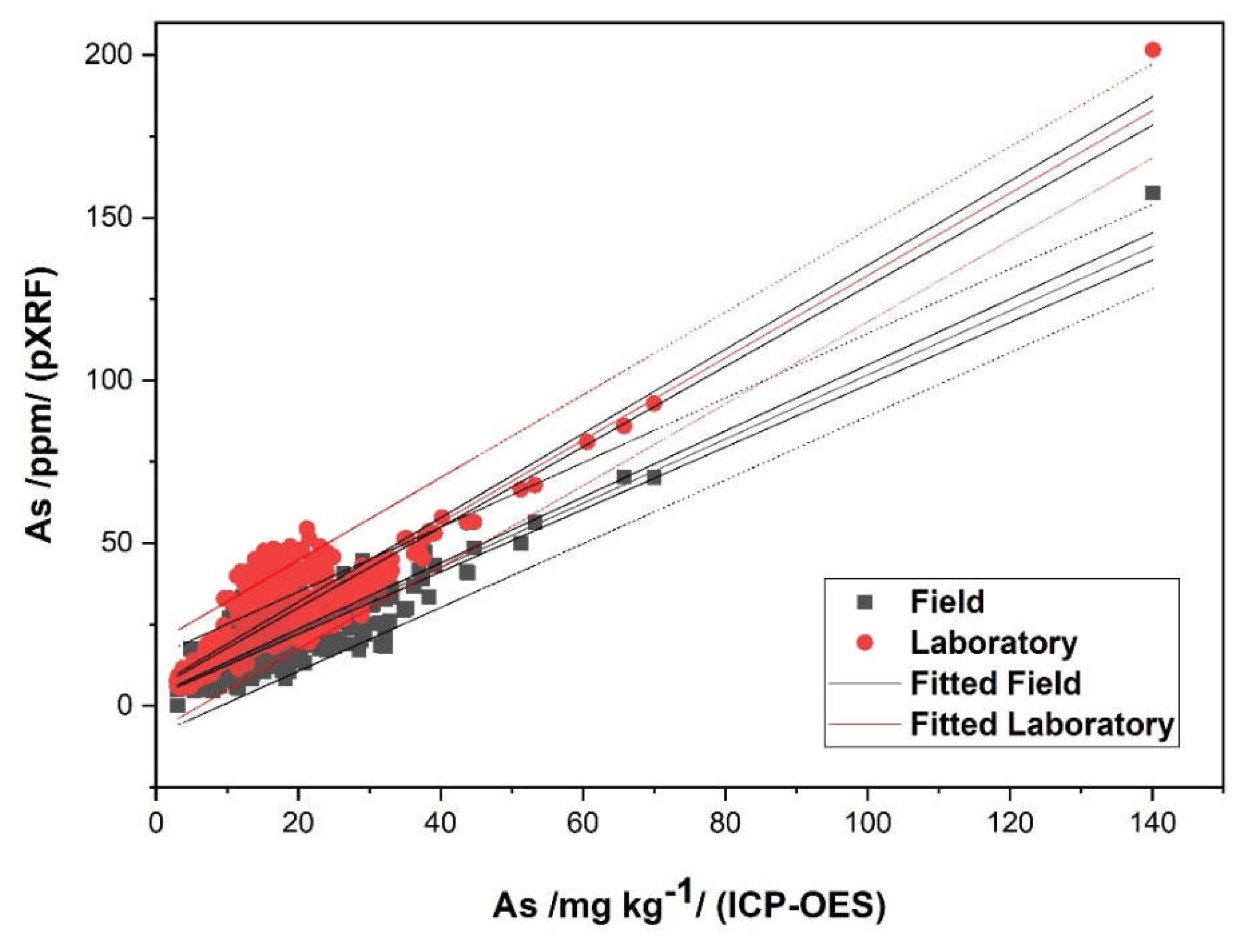
3.1. Model for Arsen (As)

The equation of the straight line relating As (FIELD) and As (ICP-OES) is estimated as: As (FIELD) = (3.1376) + (0.9859) * As (ICP-OES) using the 432 observations in this dataset. The y-intercept, the estimated value of As (FIELD) when As (ICP-OES) is zero, is 3.1376, with a standard error of 0.5843. The slope, the estimated change in As (Field) per unit change in As (ICP-OES), is 0.9859, with a standard error of 0.0290. The value of R-Squared, the proportion of the variation in As (FIELD) that can be accounted for by variation in As (ICP-OES), is 0.7295. The correlation between As (FIELD) and As (ICP-OES) is 0.8541. The estimated slope is 0.9859. The lower limit of the 95% confidence interval for the slope is 0.9290 and the upper limit is 1.0428. The estimated intercept is 3.1376. The lower limit of the 95% confidence interval for the intercept is 1.9891 and the upper limit is 4.2861.
The equation of the straight line relating As (LABORATORY) and As (ICP-OES) is estimated as: As (LABORATORY) = (5.7511) + (1.2647) * As (ICP-OES) using the 459 observations in this dataset. The y-intercept value, the slope, the Residual Sum of Squares, the Pearson’s r, the R2 value, and the MEP and AIC values are shown in Table 1. The lower limit of the 95% confidence interval for the intercept is 4.5581 and the upper limit is 6.9440 (Figure 1).

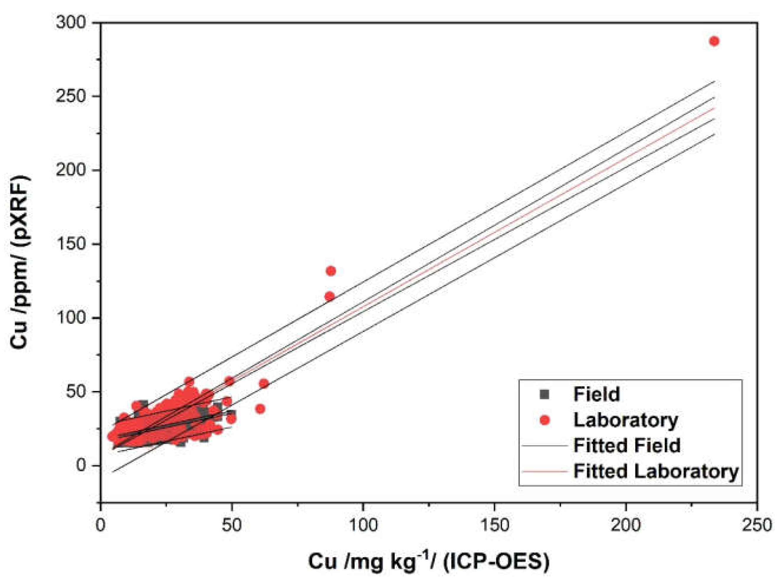
3.2. Model for Copper (Cu)

The equation of the straight line relating Cu (FIELD) and Cu (ICP-OES) is estimated as: Cu (FIELD) = (17.1506) + (0.3843) * Cu (ICP-OES) using the 264 observations in this dataset. The y-intercept value, the slope, the Residual Sum of Squares, the Pearson’s r, the R2 value, and the MEP and AIC values are shown in Table 1. The lower limit of the 95% confidence interval for the intercept is 15.3500 and the upper limit is 18.9513.
The equation of the straight line relating Cu (LABORATORY) and Cu (ICP-OES) is estimated as: Cu (LABORATORY) = (6.9702) + (1.0072) * Cu (ICP-OES) using the 328 observations in this dataset. The y-intercept value, the slope, the Residual Sum of Squares, the Pearson’s r, the R2 value, and the MEP and AIC values are shown in Table 1. The lower limit of the 95% confidence interval for the intercept is 5.4402 and the upper limit is 8.5002 (Figure 2).

3.3. Model for Manganese (Mn)

The equation of the straight line relating Mn (FIELD) and Mn (ICP–OES) is estimated as: Mn (FIELD) = (62.7329) + (0.6874) * Mn (ICP–OES) using the 450 observations in this dataset. The y-intercept value, the slope, the Residual Sum of Squares, the Pearson’s r, the R2 value, and the MEP and AIC values are shown in Table 1. The lower limit of the 95% confidence interval for the intercept is 31.9191 and the upper limit is 93.5467.
The equation of the straight line relating Mn (LABORATORY) and Mn (ICP-OES) is estimated as: Mn (LABORATORY) = (93.0551) + (1.1388) * Mn (ICP-OES) using the 473 observations in this dataset. The y-intercept value, the slope, the Residual Sum of Squares, the Pearson’s r, the R2 value, and the MEP and AIC values are shown in Table 1. The lower limit of the 95% confidence interval for the intercept is 58.2313 and the upper limit is 127.8790 (Figure 3).

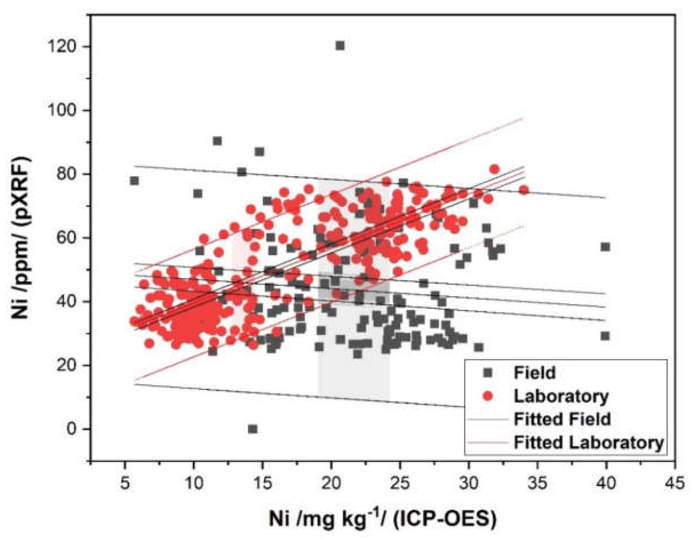
3.4. Model for Nickel (Ni)

The equation of the straight line relating Ni (FIELD) and Ni (ICP-OES) is estimated as: Ni (FIELD) = (49.9096) + (−0.2900) * Ni (ICP-OES) using the 140 observations in this dataset. The y-intercept value, the slope, the Residual Sum of Squares, the Pearson’s r, the R2 value, and the MEP and AIC values are shown in Table 1. The lower limit of the 95% confidence interval for the intercept is 39.0973 and the upper limit is 60.7219.
The equation of the straight line relating Ni (LABORATORY) and Ni (ICP-OES) is estimated as: Ni (LABORATORY) = (22.4618) + (1.7133) * Ni (ICP-OES) using the 303 observations in this dataset. The y-intercept value, the slope, the Residual Sum of Squares, the Pearson’s r, the R2 value, and the MEP and AIC values are shown in Table 1. The lower limit of the 95% confidence interval for the intercept is 20.0533 and the upper limit is 24.8702 (Figure 4).

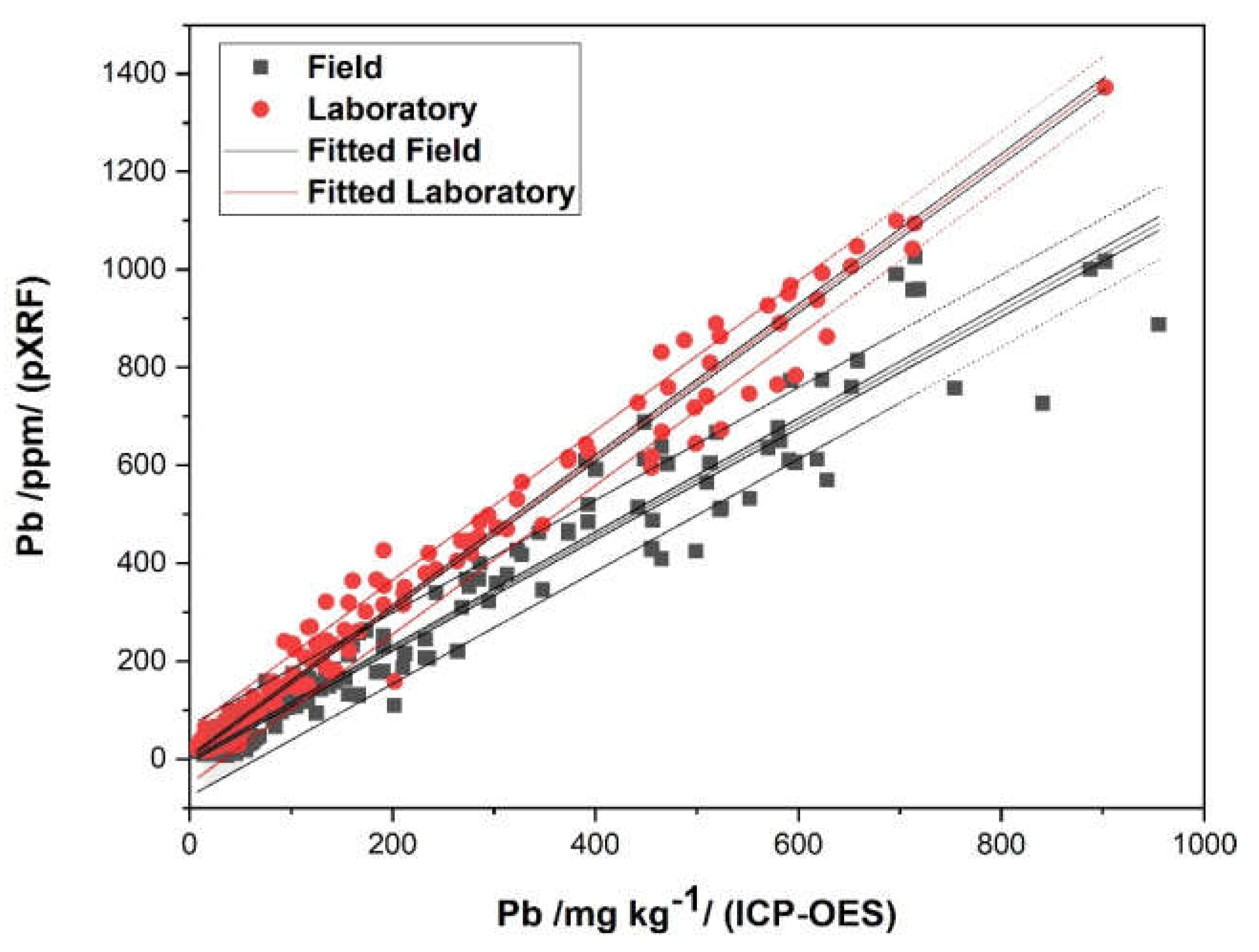
3.5. Model for Lead (Pb)

The equation of the straight line relating Pb (FIELD) and Pb (ICP-OES) is estimated as: Pb (FIELD) = (−3.6965) + (1.1493) * Pb (ICP–OES) using the 489 observations in this dataset. The y-intercept value, the slope, the Residual Sum of Squares, the Pearson’s r, the R2 value, and the MEP and AIC values are shown in Table 1. The lower limit of the 95% confidence interval for the intercept is −7.4642 and the upper limit is 0.0711.
The equation of the straight line relating Pb (LABORATORY) and Pb (ICP-OES) is estimated as: Pb (LABORATORY) = (4.4310) + (1.5266) * Pb (ICP-OES) using the 484 observations in this dataset. The y-intercept value, the slope, the Residual Sum of Squares, the Pearson’s r, the R2 value, and the MEP and AIC values are shown in Table 1. The lower limit of the 95% confidence interval for the intercept is 1.5284 and the upper limit is 7.3336 (Figure 5).

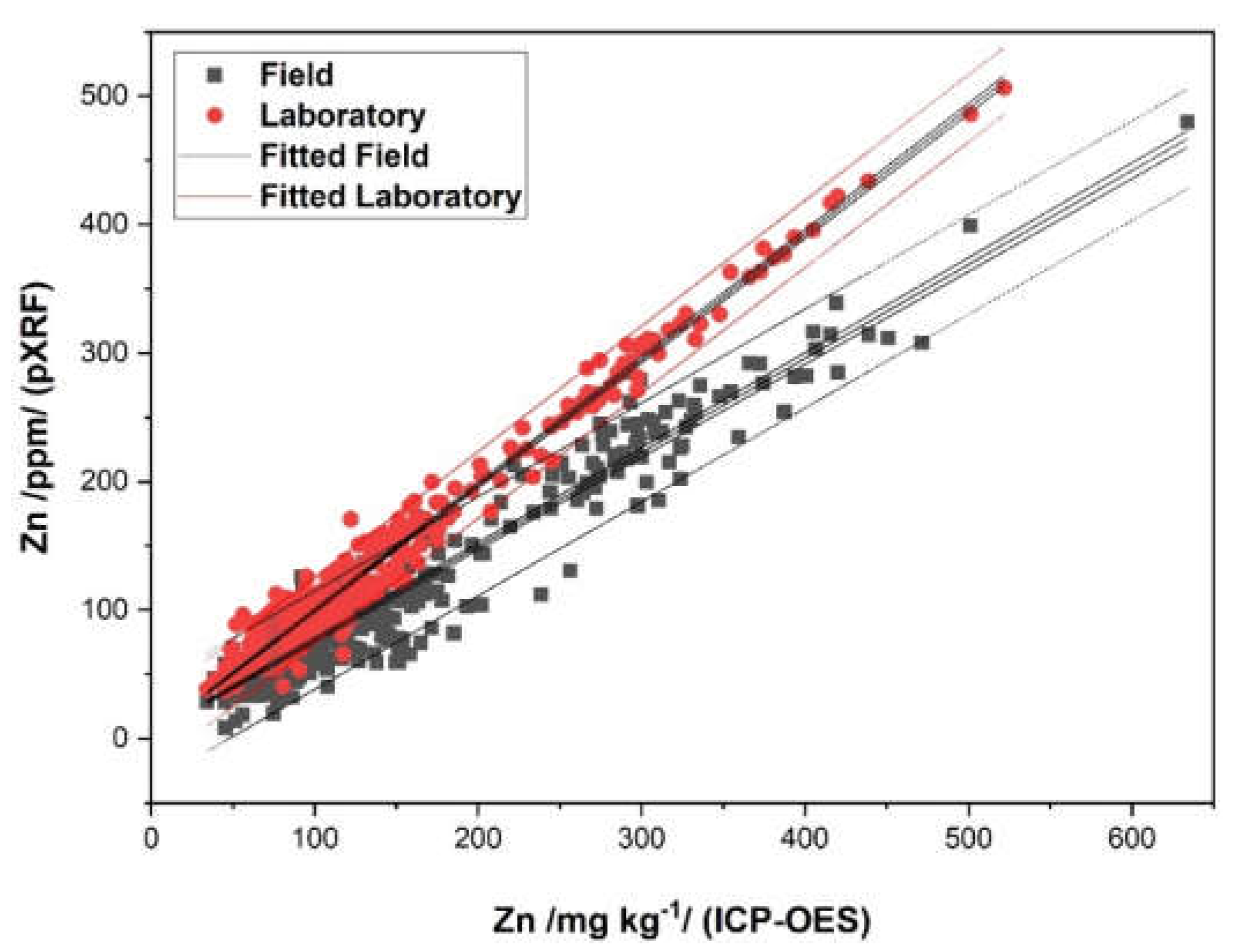
3.6. Model for Zinc (Zn)

The equation of the straight line relating Zn (FIELD) and Zn (ICP-OES) is estimated as: Zn (FIELD) = (3.5548) + (0.7307) * Zn (ICP-OES) using the 478 observations in this dataset. The y-intercept value, the slope, the Residual Sum of Squares, the Pearson’s r, the R2 value, and the MEP and AIC values are shown in Table 1. The lower limit of the 95% confidence interval for the intercept is 0.4752 and the upper limit is 6.6344.
The equation of the straight line relating Zn (LABORATORY) and Zn (ICP-OES) is estimated as: Zn (LABORATORY) = (2.0281) + (0.9766) * Zn (ICP-OES) using the 468 observations in this dataset. The y-intercept value, the slope, the Residual Sum of Squares, the Pearson’s r, the R2 value, and the MEP and AIC values are shown in Table 1. The lower limit of the 95% confidence interval for the intercept is −0.1683 and the upper limit is 4.2245 (Figure 6).

3.7. Model Summary

The equations of the lines for the individual risk elements (As, Cu, Mn, Ni, Pb, Zn), with a detailed statistical evaluation, are given in Figure 1, Figure 2, Figure 3, Figure 4, Figure 5 and Figure 6. The models were processed by regression triplet (data critique, model critique and methods in regression triplet). Therefore, the parameters Mean Prediction Error (MEP) and AAkaike information criterion (AIC) are given in each model. The smaller the AIC or MEP, the more suitable the model. The number of repetitions in single datasets ranges from 140 to 489. The coefficients of determination (R2) were 0.96 (Pb), 0.92 (Zn), 0.72 (As), 0.63 (Mn), 0.31 (Cu) and 0.01 (Ni) for in situ measuring (FIELD). For laboratory measurements using the pXRF (LABORATORY), the coefficients were 0.99 (Pb), 0.98 (Zn), 0.89 (Cu, Mn), 0.88 (As) and 0.81 (Ni). All models, except the Ni model (FIELD), were statistically significant (Fisher-Snedecor test) and correct (Scott’s multicollinearity criterion). By comparing FIELD and LABORATORY measurements to ICP-OES, a higher tightness of relationships was always recorded between LABORATORY and ICP-OES. For in situ analysis of Ni and Cu concentrations in the soil, the use of pXRF is problematic (R2 for Ni = 0.01, R2 for Cu = 0.31). On the contrary, for Pb and Zn, the results are excellent, both for in situ (FIELD) and for LABORATORY measurements (R2 higher than 0.9).
Cu, Mn and As show a worse dependence in the models (R2 = 0.75–0.90) than Pb and Zn; however, the pXRF is suitable for orientational survey of environmental quality (assuming analysis in laboratory conditions—LABORATORY). Based on the model, the in situ (FIELD) analysis of Mn and As, as well as Ni in the laboratory (LABORATORY), is suitable for approximate estimation.

4. Discussion

The most important parameter observed when comparing the results obtained with pXRF and laboratory methods is the coefficient of determination, (R2). According to the United States Environmental Protection Agency, the results of the analysis obtained by pXRF are divided into three categories, depending on R2: (1) definitive, (2) quantitative screening, and (3) qualitative screening. The R2 parameter is based on the regression between pXRF and the reference data. The range of parameter R2 for individual categories is as follows: (1) 0.85–1, (2) 0.70–0.85, and (3) <70 [52,53]. When comparing pXRF results obtained from in situ measurements (FIELD) and in-laboratory conditions (LABORATORY), a higher dependence (tightness of the relationship) with the standard laboratory method (ICP-OES) has always been demonstrated by LABORATORY results (see Model Summary). Our results from in situ measurements are similar to the study of Qu et al. [54]. In this paper, pXRF was used to analyse an area of 60 km2 (agricultural area of Wuhan, Hubei, China), with a soil depth of 20 cm, achieving a correlation coefficient of R2 = 0.95 for Pb compared to the laboratory method. Similar correlation coefficients for the determination of risk elements using a pXRF, by directly measuring in the field, were also reported by Hu et al. [15], Ran et al. [55], Caporale et al. [48], Zhou et al. [56]; Qu et al. [57]; Kennedy, Kelloway [58].
The accuracy of measuring the concentration of risk elements in the soil will increase if we use pXRF in the laboratory. In this case, the soil samples are sieved, dried and homogenized before the analysis [32]. This step is identical to the preparation of samples for spectroscopic analysis. The prepared soil samples are then poured into plastic capsules. The measurement itself is performed in a stand to which pXRF is attached. However, the increase in sensitivity is redeemed by labor and time. Depending on the number of samples, the analysis may take several days. Our measurements can confirm this, as we achieved higher coefficients of determination in the laboratory (Model Summary). Similar results were published by Wan et al. [32], who analysed agricultural soil around Kunming City, Yunnan Province, southwestern China, and compared the pXRF results measured in the laboratory and then by ICP-MS. Our results are also consistent with the study published by Adler et al. [59]. In this study, a total of 1833 agricultural soil samples in Sweden were analysed and the R2 coefficients for the elements Cu, Cd and Zn ranged from 0.63 to 0.92. In the case of As, our results are consistent with the results of a study published by Kebonye et al. [60]. In this study, alluvial soil (Fluvisols and Graysols with grass cover) from the Litavka river area, Příbram, the Czech Republic, was measured in the laboratory using the pXRF. This soil is one of the most polluted flood soils in Europe [61]. The use of pXRF in laboratory conditions highlighted the effect of soil moisture, especially for the Ni element (compared to other elements). While in situ measurements could be described as inapplicable or problematic, sample treatment significantly increased the accuracy of the determination.
Based on our research and comparing the results published by other scientists in scientific articles, we can state that measuring the concentration of risk elements in agricultural land using pXRF can provide high-quality (accurate) results, in real time and very quickly (application of precision agriculture principles—efficiency, accuracy and speed [45,48,59,62,63]. pXRF offers a great opportunity for the preliminary monitoring of locally and potentially contaminated soils, followed by standard laboratory analysis [64]. (Kim and Choi 2017). pXRF instruments can also find application in the prediction of soil and soil environment properties, such as pH, carbon content and accessible nutrients [32,35,65,66].

5. Conclusions

Using the method of construction of the regression model by regression triplet (data critique, model critique and methods in regression triplet), we compared the concentrations of risk elements in alluvial soils in the basin of two rivers (Mže and Otava). The criteria r (Pearson’s r), R2 (coefficient of determination), MEP and AIC were taken into account in the construction of each model for field results.
The results measured by pXRF (in situ and in the laboratory conditions) were compared with the results obtained by ICP-OES. The number of replicates for individual risk elements ranged from 140 to 489. The coefficients of determination (R2) between pXRF in situ and ICP-OES were Pb (0.96), Zn (0.92), As (0.72), Mn (0.63), Cu (0.31) and Ni (0.01). The coefficients of determination between pXRF (in the laboratory) and ICP-OES were Pb (0.99), Zn (0.98), Cu and Mn (0.89), As (0.88) and Ni (0.81). Compared to the standard laboratory method (ICP-OES), a higher tightness of the relationship was always recorded in the case of pXRF laboratory analysis (the accuracy of the in situ pXRF determination was lower).
The use of portable XRF analysers offers faster and simpler analysis than the standard laboratory methods. Speed and simplicity are redeemed by lower accuracy. The accuracy of the determination can be easily increased by the soil sample preparation (drying, grinding, homogenization), followed by pXRF measurement in the laboratory. This method of analysis offers high-quality information on the concentrations of risk elements in the soils.

Author Contributions

Conceptualization, L.M. and L.H.; methodology, L.M., L.H., P.N. and E.K.; software, L.M., L.H.; validation, L.M.; formal analysis, L.M.; investigation, L.M., L.H.; resources, L.M., L.H.; data curation, L.M.; writing—original draft preparation, L.M., L.H.; writing—review and editing, L.M., L.H.; visualization, L.M.; supervision, E.K.; project administration, E.K.; funding acquisition, E.K. All authors have read and agreed to the published version of the manuscript.

Funding

The study was created thanks to the support of the international project No. 146 “Occurrence of hazardous elements and substances in floodplain soils in historical ore mining areas in eastern Bavaria and the Czech Republic” and research program of the Ministry of Agriculture of the Czech Republic—RO0418.

Institutional Review Board Statement

Not applicable.

Informed Consent Statement

Not applicable.

Data Availability Statement

Data sharing not applicable.

Acknowledgments

Thanks go to Peter Ivičic, Vlastimil Basař, Dana Večeřová and Miroslava Pechová for technical support and provision of field work and laboratory analyses within the project solution.

Conflicts of Interest

The authors declare no conflict of interest.

References

  1. Ren, B.; Wu, Y.; Deng, D.; Tang, X.; Li, H. Effect of multiple factors on the adsorption of Cd in an alluvial soil from Xiba, China. J. Contam. Hydrol. 2020. [Google Scholar] [CrossRef]
  2. Li, C.; Sanchez, G.M.; Wu, Z.; Cheng, J.; Zhang, S.; Wang, Q.; Li, F.; Sun, G.; Meentemeyer, R.K. Spatiotemporal patterns and drivers of soil contamination with heavy metals during an intensive urbanization period (1989–2018) in southern China. Environ. Pollut. 2020, 260. [Google Scholar] [CrossRef]
  3. Lal, R. Soil organic matter content and crop yield. J. Soil Water Conserv. 2020, 75, 27A–32A. [Google Scholar] [CrossRef] [Green Version]
  4. Shokr, M.S.; El Baroudy, A.A.; Fullen, M.A.; El-Beshbeshy, T.R.; Ali, R.R.; Elhalim, A.; Guerra, A.J.T.; Jorge, M.C.O. Mapping of heavy metal contamination in alluvial soils of the Middle Nile Delta of Egypt. J. Environ. Eng. Landsc. Manag. 2016, 24, 218–231. [Google Scholar] [CrossRef]
  5. Bajčan, D.; Hegedusova, A.; Šnirc, M.; Trebichalský, P.; Jančo, I. The Impact of Former Mining Activities on the Contamination of Alluvial Soils in the Region Hont. In Proceedings of the 19th International Multidisciplinary Scientific GeoConference SGEM 2019, Albena, Bulgaria, 28 June–6 July 2019; pp. 499–506. [Google Scholar]
  6. Barman, M.; Datta, S.P.; Rattan, R.K.; Meena, M.C. Critical Limits of Deficiency of Nickel in Intensively Cultivated Alluvial Soils. J. Soil Sci. Plant Nutr. 2020, 20, 284–292. [Google Scholar] [CrossRef]
  7. Adimalla, N. Heavy metals pollution assessment and its associated human health risk evaluation of urban soils from Indian cities: A review. Environ. Geochem. Health 2020, 42, 173–190. [Google Scholar] [CrossRef] [PubMed]
  8. Karande, U.B.; Kadam, A.; Umrikar, B.N.; Wagh, V.; Sankhua, R.N.; Pawar, N.J. Environmental modelling of soil quality, heavy-metal enrichment and human health risk in sub-urbanized semiarid watershed of western India. Model. Earth Syst. Environ. 2020, 6, 545–556. [Google Scholar] [CrossRef]
  9. Kaur, M.; Kumar, A.; Mehra, R.; Kaur, I. Quantitative assessment of exposure of heavy metals in groundwater and soil on human health in Reasi district, Jammu and Kashmir. Environ. Geochem. Health 2020, 42, 77–94. [Google Scholar] [CrossRef]
  10. Rostami, S.; Kamani, H.; Shahsavani, S.; Hoseini, M. Environmental monitoring and ecological risk assessment of heavy metals in farmland soils: Ecological risk assessment of heavy metals in Kamfiruz district. Hum. Ecol. Risk Assess. 2020, 1–13. [Google Scholar] [CrossRef]
  11. Shaheen, S.M.; Antoniadis, V.; Kwon, E.; Song, H.; Wang, S.L.; Hseu, Z.Y.; Rinklebe, J. Soil contamination by potentially toxic elements and the associated human health risk in geo- and anthropogenic contaminated soils: A case study from the temperate region (Germany) and the arid region (Egypt). Environ. Pollut. 2020, 262, 114212. [Google Scholar] [CrossRef]
  12. Fazekašová, D.; Fazekaš, J. Soil Quality and Heavy Metal Pollution Assessment of Iron Ore Mines in Nizna Slana (Slovakia). Sustainability 2020, 12, 2549. [Google Scholar] [CrossRef] [Green Version]
  13. Sparks, D.L.; Page, A.L.; Helmke, P.A.; Loeppert, R.H.; Soltanpour, P.N.; Tabatabai, M.A.; Johnston, C.T.; Sumner, M.E. (Eds.) Methods of Soil Analysis; SSSA Book Series; Soil Science Society of America, American Society of Agronomy: Madison, WI, USA, 1996; ISBN 9780891188667. [Google Scholar]
  14. Bettinelli, M.; Beone, G.; Spezia, S.; Baffi, C. Determination of heavy metals in soils and sediments by microwave-assisted digestion and inductively coupled plasma optical emission spectrometry analysis. Anal. Chim. Acta 2000, 424, 289–296. [Google Scholar] [CrossRef]
  15. Hu, W.; Huang, B.; Weindorf, D.C.; Chen, Y. Metals analysis of agricultural soils via portable X-ray fluorescence spectrometry. Bull. Environ. Contam. Toxicol. 2014, 92, 420–426. [Google Scholar] [CrossRef] [PubMed]
  16. Bonelli, M.G.; Ferrini, M.; Manni, A. Artificial neural networks to evaluate organic and inorganic contamination in agricultural soils. Chemosphere 2017, 186, 124–131. [Google Scholar] [CrossRef]
  17. Al Maliki, A.; Al-lami, A.K.; Hussain, H.M.; Al-Ansari, N. Comparison between inductively coupled plasma and X-ray fluorescence performance for Pb analysis in environmental soil samples. Environ. Earth Sci. 2017, 76, 433. [Google Scholar] [CrossRef] [Green Version]
  18. Wang, B.; Yu, J.; Huang, B.; Hu, W.; Chang, Q. Fast Monitoring Soil Environmental Qualities of Heavy Metal by Portable X-ray Fluorescence Spectrometer. Spectrosc. Spectr. Anal. 2015, 35, 1735–1740. [Google Scholar] [CrossRef]
  19. Rouillon, M.; Taylor, M.P. Can field portable X-ray fluorescence (pXRF) produce high quality data for application in environmental contamination research? Environ. Pollut. 2016, 214, 255–264. [Google Scholar] [CrossRef]
  20. Konstantinova, E.; Minkina, T.; Nevidomskaya, D.; Mandzhieva, S.; Bauer, T.; Zamulina, I.; Burachevskaya, M.; Sushkova, S. Exchangeable form of potentially toxic elements in floodplain soils along the river-marine systems of Southern Russia. Eurasian J. Soil Sci. 2021, 10, 132–141. [Google Scholar] [CrossRef]
  21. Hu, B.; Chen, S.; Hu, J.; Xia, F.; Xu, J.; Li, Y.; Shi, Z. Application of portable XRF and VNIR sensors for rapid assessment of soil heavy metal pollution. PLoS ONE 2017, 12, e0172438. [Google Scholar] [CrossRef] [PubMed] [Green Version]
  22. Hunt, A.M.W.; Speakman, R.J. Portable XRF analysis of archaeological sediments and ceramics. J. Archaeol. Sci. 2015, 53, 626–638. [Google Scholar] [CrossRef]
  23. Rincheval, M.; Cohen, D.R.; Hemmings, F.A. Biogeochemical mapping of metal contamination from mine tailings using field-portable XRF. Sci. Total Environ. 2019, 662, 404–413. [Google Scholar] [CrossRef]
  24. McIntosh, K.G.; Guimarães, D.; Cusack, M.J.; Vershinin, A.; Chen, Z.W.; Yang, K.; Parsons, P.J. Evaluation of portable XRF instrumentation for assessing potential environmental exposure to toxic elements. Int. J. Environ. Anal. Chem. 2016, 96, 15–37. [Google Scholar] [CrossRef] [PubMed]
  25. Melquiades, F.L.; Appoloni, C.R. Application of XRF and field portable XRF for environmental analysis. J. Radioanal. Nucl. Chem. 2004, 262, 533–541. [Google Scholar] [CrossRef]
  26. Peinado, F.M.; Ruano, S.M.; González, M.G.B.; Molina, C.E. A rapid field procedure for screening trace elements in polluted soil using portable X-ray fluorescence (PXRF). Geoderma 2010, 159, 76–82. [Google Scholar] [CrossRef]
  27. Kodom, K.; Preko, K.; Boamah, D. X-ray Fluorescence (XRF) Analysis of Soil Heavy Metal Pollution from an Industrial Area in Kumasi, Ghana. Soil Sediment Contam. 2012, 21, 1006–1021. [Google Scholar] [CrossRef]
  28. Parsons, C.; Margui Grabulosa, E.; Pili, E.; Floor, G.H.; Roman-Ross, G.; Charlet, L. Quantification of trace arsenic in soils by field-portable X-ray fluorescence spectrometry: Considerations for sample preparation and measurement conditions. J. Hazard. Mater. 2013, 262, 1213–1222. [Google Scholar] [CrossRef] [PubMed]
  29. Rinklebe, J.; Antoniadis, V.; Shaheen, S.M.; Rosche, O.; Altermann, M. Health risk assessment of potentially toxic elements in soils along the Central Elbe River, Germany. Environ. Int. 2019, 126, 76–88. [Google Scholar] [CrossRef] [PubMed]
  30. Paveley, C.F.; Davies, B.E.; Jones, K. Comparison of results obtained by X-ray fluorescence of the total soil and the atomic absorption spectrometry assay of an acid digest in the routine determination of lead and zinc in soils. Commun. Soil Sci. Plant Anal. 1988, 19, 107–116. [Google Scholar] [CrossRef]
  31. Jenkins, R. X-ray Fluorescence Spectrometry, 2nd ed.; Wiley-VCH: Weinheim, Germany, 1999; ISBN 978-1-118-52104-5. [Google Scholar]
  32. Wan, M.; Hu, W.; Qu, M.; Tian, K.; Zhang, H.; Wang, Y.; Huang, B. Application of arc emission spectrometry and portable X-ray fluorescence spectrometry to rapid risk assessment of heavy metals in agricultural soils. Ecol. Indic. 2019, 101, 583–594. [Google Scholar] [CrossRef]
  33. Lilli, M.A.; Moraetis, D.; Nikolaidis, N.P.; Karatzas, G.P.; Kalogerakis, N. Characterization and mobility of geogenic chromium in soils and river bed sediments of Asopos basin. J. Hazard. Mater. 2015, 281, 12–19. [Google Scholar] [CrossRef] [PubMed]
  34. Ding, L.; Wang, S.; Cai, B.; Zhang, M.; Qu, C. Application of portable X-ray fluorescence spectrometry in environmental investigation of heavy metal-contaminated sites and comparison with laboratory analysis. IOP Conf. Ser. Earth Environ. Sci. 2018, 121, 10. [Google Scholar] [CrossRef]
  35. Horta, A.; Malone, B.; Stockmann, U.; Minasny, B.; Bishop, T.F.A.; McBratney, A.B.; Pallasser, R.; Pozza, L. Potential of integrated field spectroscopy and spatial analysis for enhanced assessment of soil contamination: A prospective review. Geoderma 2015, 241–242, 180–209. [Google Scholar] [CrossRef] [Green Version]
  36. Sahraoui, H.; Hachicha, M. Effect of soil moisture on trace elements concentrations. J. Fundam. Appl. Sci. 2017, 9, 468–484. [Google Scholar] [CrossRef] [Green Version]
  37. Padilla, J.T.; Hormes, J.; Magdi Selim, H. Use of portable XRF: Effect of thickness and antecedent moisture of soils on measured concentration of trace elements. Geoderma 2019, 337, 143–149. [Google Scholar] [CrossRef]
  38. Stockmann, U.; Cattle, S.R.; Minasny, B.; McBratney, A.B. Utilizing portable X-ray fluorescence spectrometry for in-field investigation of pedogenesis. Catena 2016, 139, 220–231. [Google Scholar] [CrossRef]
  39. U.S. EPA. Method 6200: Field Portable X-ray Fluorescence Spectrometry for the Determination of Elemental Concentrations in Soil and Sediment; United States Environmental Protection Agency: Washington, DC, USA, 2007.
  40. Menšík, L.; Hlisnikovský, L.; Holík, L.; Nerušil, P.; Kunzová, E. Possibilities of determination of risk elements in alluvial agriculture soils in the MŽE and otava river basins by X-ray fluorescence spectrometry. Agriculture 2020, 66, 15–23. [Google Scholar] [CrossRef]
  41. Laiho, J.; Perämäki, P. Evaluation of portable X-ray fluorescence (PXRF) sample preparation methods. Spec. Pap. Geol. Surv. Finl. 2005, 73–82. [Google Scholar]
  42. Stockmann, U.; Jang, H.J.; Minasny, B.; McBratney, A.B. The Effect of Soil Moisture and Texture on Fe Concentration Using Portable X-ray Fluorescence Spectrometers. In Digital Soil Morphometrics; Springer: Cham, Switzerland, 2016; pp. 63–71. [Google Scholar] [CrossRef]
  43. Hangen, E.; Čermák, P.; Geuß, U.; Hlisnikovský, L. Information depth of elements affects accuracy of parallel pXRF in situ measurements of soils. Environ. Monit. Assess. 2019, 191. [Google Scholar] [CrossRef]
  44. Radu, T.; Diamond, D. Comparison of soil pollution concentrations determined using AAS and portable XRF techniques. J. Hazard. Mater. 2009, 171, 1168–1171. [Google Scholar] [CrossRef] [PubMed]
  45. McComb, J.Q.; Rogers, C.; Han, F.X.; Tchounwou, P.B. Rapid screening of heavy metals and trace elements in environmental samples using portable X-ray fluorescence spectrometer, A comparative study. Water Air Soil Pollut. 2014, 225. [Google Scholar] [CrossRef] [PubMed] [Green Version]
  46. Lee, H.; Choi, Y.; Suh, J.; Lee, S.H. Mapping copper and lead concentrations at abandoned mine areas using element analysis data from ICP-AES and portable XRF instruments: A comparative study. Int. J. Environ. Res. Public Health 2016, 13, 384. [Google Scholar] [CrossRef] [PubMed]
  47. Schneider, A.R.; Cancès, B.; Breton, C.; Ponthieu, M.; Morvan, X.; Conreux, A.; Marin, B. Comparison of field portable XRF and aqua regia/ICPAES soil analysis and evaluation of soil moisture influence on FPXRF results. J. Soils Sediments 2016, 16, 438–448. [Google Scholar] [CrossRef]
  48. Caporale, A.G.; Adamo, P.; Capozzi, F.; Langella, G.; Terribile, F.; Vingiani, S. Monitoring metal pollution in soils using portable-XRF and conventional laboratory-based techniques: Evaluation of the performance and limitations according to metal properties and sources. Sci. Total Environ. 2018, 643, 516–526. [Google Scholar] [CrossRef]
  49. IUSS Working Group WRB. World Reference Base for Soil Resources 2014, Update 2015 International Soil Classification System for Naming Soils and Creating Legends for Soil Maps; World Soil Resources Reports No. 106; FAO (Food and Agriculture Organization of the United Nations): Rome, Italy, 2015. [Google Scholar]
  50. Zbíral, J. Soil Analysis. Standard Working Procedures; Central Institute for Supervising and Testing in Agriculture: Brno, Czech Republic, 2011; ISBN 9788074010408. [Google Scholar]
  51. Melou, M.; Militký, J. Statistical Data Analysis, a Practical Guide with 1250 Exercises and Answer Key on CD; Woodhead Publishing: New Delhi, India, 2012; ISBN 9780857091093. [Google Scholar]
  52. Hess, E.; Splichal, P. Environmental Technology Verification Report: Field Portable X-ray Fluorescence Analyzer: Scitec MAP Spectrum Analyzer (EPA 600-R-97-147; NERL-LV-98-012; PB2001101792); U.S. Environmental Protection Agency: Washington, DC, USA, 1998.
  53. Messager, M.L.; Davies, I.P.; Levin, P.S. Development and validation of in-situ and laboratory X-ray fluorescence (XRF) spectroscopy methods for moss biomonitoring of metal pollution. MethodsX 2021, 8, 101319. [Google Scholar] [CrossRef]
  54. Qu, M.; Chen, J.; Li, W.; Zhang, C.; Wan, M.; Huang, B.; Zhao, Y. Correction of in-situ portable X-ray fluorescence (PXRF) data of soil heavy metal for enhancing spatial prediction. Environ. Pollut. 2019, 254, 112993. [Google Scholar] [CrossRef]
  55. Ran, J.; Wang, D.; Wang, C.; Zhang, G.; Yao, L. Using portable X-ray fluorescence spectrometry and GIS to assess environmental risk and identify sources of trace metals in soils of peri-urban areas in the Yangtze Delta region, China. Environ. Sci. Process. Impacts 2014, 16, 1870–1877. [Google Scholar] [CrossRef]
  56. Zhou, S.; Yuan, Z.; Cheng, Q.; Zhang, Z.; Yang, J. Rapid in situ determination of heavy metal concentrations in polluted water via portable XRF: Using Cu and Pb as example. Environ. Pollut. 2018, 243, 1325–1333. [Google Scholar] [CrossRef] [PubMed]
  57. Qu, M.; Chen, J.; Huang, B.; Zhao, Y. Resampling with in situ field portable X-ray fluorescence spectrometry (FPXRF) to reduce the uncertainty in delineating the remediation area of soil heavy metals. Environ. Pollut. 2021, 271, 116310. [Google Scholar] [CrossRef]
  58. Kennedy, S.A.; Kelloway, S.J. Heavy Metals in Archaeological Soils. Adv. Archaeol. Pract. 2021, 1–15. [Google Scholar] [CrossRef]
  59. Adler, K.; Piikki, K.; Söderström, M.; Eriksson, J.; Alshihabi, O. Predictions of Cu, Zn, and Cd Concentrations in Soil Using Portable X-ray Fluorescence Measurements. Sensors 2020, 20, 474. [Google Scholar] [CrossRef] [Green Version]
  60. Kebonye, N.M.; John, K.; Chakraborty, S.; Agyeman, P.C.; Ahado, S.K.; Eze, P.N.; Němeček, K.; Drábek, O.; Borůvka, L. Comparison of multivariate methods for arsenic estimation and mapping in floodplain soil via portable X-ray fluorescence spectroscopy. Geoderma 2021, 384, 114792. [Google Scholar] [CrossRef]
  61. Boruvka, L.; Vacha, R. Litavka River Alluvium as a Model Area Heavily Polluted with Potentially Risk Elements. In Phytoremediation of Metal-Contaminated Soils; Kluwer Academic Publishers: Dordrecht, The Netherlands, 2006; pp. 267–298. [Google Scholar]
  62. Shuttleworth, E.L.; Evans, M.G.; Hutchinson, S.M.; Rothwell, J.J. Assessment of lead contamination in peatlands using field portable XRF. Water Air. Soil Pollut. 2014, 225. [Google Scholar] [CrossRef]
  63. Havukainen, J.; Hiltunen, J.; Puro, L.; Horttanainen, M. Applicability of a field portable X-ray fluorescence for analyzing elemental concentration of waste samples. Waste Manag. 2019, 83, 6–13. [Google Scholar] [CrossRef]
  64. Kim, S.M.; Choi, Y. Assessing statistically significant heavy-metal concentrations in abandoned mine areas via hot spot analysis of portable XRF data. Int. J. Environ. Res. Public Health 2017, 14, 16. [Google Scholar] [CrossRef] [Green Version]
  65. Nawar, S.; Delbecque, N.; Declercq, Y.; De Smedt, P.; Finke, P.; Verdoodt, A.; Van Meirvenne, M.; Mouazen, A.M. Can spectral analyses improve measurement of key soil fertility parameters with X-ray fluorescence spectrometry? Geoderma 2019, 350, 29–39. [Google Scholar] [CrossRef]
  66. Andrade, R.; Faria, W.M.; Silva, S.H.G.; Chakraborty, S.; Weindorf, D.C.; Mesquita, L.F.; Guilherme, L.R.G.; Curi, N. Prediction of soil fertility via portable X-ray fluorescence (pXRF) spectrometry and soil texture in the Brazilian Coastal Plains. Geoderma 2020, 357, 113960. [Google Scholar] [CrossRef]
Figure 1. Statistical significance of regression model for Arsen (pXRF) in soil samples from experimental soil sites from Otava and Mže river basins measured in FIELD and LABORATORY.
Agronomy 11 00938 g001
Figure 2. Statistical significance of regression model for Copper (pXRF) in soil samples from experimental soil sites from Otava and Mže river basins, measured in FIELD and LABORATORY.
Agronomy 11 00938 g002
Figure 3. Statistical significance of regression model for Manganese (pXRF) in soil samples from experimental soil sites from Otava and Mže river basins measured in FIELD and LABORATORY.
Agronomy 11 00938 g003
Figure 4. Statistical significance of regression model for Nickel (pXRF) in soil samples from experimental soil sites from Otava and Mže river basins measured in FIELD and LABORATORY.
Agronomy 11 00938 g004
Figure 5. Statistical significance of regression model for Lead (pXRF) in soil samples from experimental soil sites from Otava and Mže river basins, measured in FIELD and LABORATORY.
Agronomy 11 00938 g005
Figure 6. Statistical significance of regression model for Zinc (pXRF) in soil samples from experimental soil sites from Otava and Mže river basins measured in FIELD and LABORATORY.
Agronomy 11 00938 g006
Table 1. Model characteristics of the pXRF–FIELD and pXRF–LABORATORY comparison for As, Cu, Mn, Ni, Pb and Zn.
As (pXRF) FIELDAs (pXRF) LABORATORYCu (pXRF) FIELDCu (pXRF) LABORATORY
Intercept3.138 ± 0.5845.751 ± 0.60717.151 ± 0.9146.970 ± 0.778
Slope0.986 ± 0.0291.265 ± 0.0310.384 ± 0.0351.007 ± 0.027
Residual Sum of Squares16,463.96422,110.3017056.46621,571.303
Pearson’s r0.8540.8870.5630.898
R20.7290.7860.3170.807
MEP39.12949.24827.1250.561
AIC1576.6981782.510871.43885.573
Mn (pXRF) FIELDMn (pXRF) LABORATORYNi (pXRF) FIELDNi (pXRF) LABORATORY
Intercept62.733 ± 15.67993.056 ± 17.72249.910 ± 5.46822.462 ± 1.224
Slope0.687 ± 0.0241.139 ± 0.027−0.290 ± 0.2441.713 ± 0.070
Residual Sum of Squares5,974,539.2381.09716 × 10−740,933.99722,037.307
Pearson’s r0.7990.892−0.1000.816
R20.6380.7960.0100.666
MEP13,375.95424,382.635-73.516
AIC4276.1964808.1535-1302.888
Pb (pXRF) FIELDPb (pXRF) LABORATORYZn (pXRF) FIELDZn (pXRF) LABORATORY
Intercept−3.697 ± 1.9184.431 ± 1.4773.554 ± 1.5672.028 ± 1.118
Slope1.149 ± 0.0101.527 ± 0.0090.731 ± 0.0100.977 ± 0.008
Residual Sum of Squares660,329.315382,461.348180,251.14180,459.575
Pearson’s r0.9810.9920.9600.986
R20.9630.9840.9220.973
MEP1408.789809.513380.689173.113
AIC3528.7763233.3922839.7332412.816
Publisher’s Note: MDPI stays neutral with regard to jurisdictional claims in published maps and institutional affiliations.

