Article

Impacts of Effects of Deficit Irrigation Strategy on Water Use Efficiency and Yield in Cotton under Different Irrigation Systems

by
Hanan H. Shukr
1,
Keith G. Pembleton
1,2,*,
Andrew F. Zull
1,3 and
Geoff J. Cockfield
1
1
Centre for Sustainable Agricultural Systems, University of Southern Queensland, Toowoomba, QLD 4350, Australia
2
School of Sciences, University of Southern Queensland, Toowoomba, QLD 4350, Australia
3
Crop and Food Science, Queensland Department of Agriculture and Fisheries, Toowoomba, QLD 4350, Australia
*
Author to whom correspondence should be addressed.
Agronomy 2021, 11(2), 231; https://doi.org/10.3390/agronomy11020231
Submission received: 11 December 2020 / Revised: 22 January 2021 / Accepted: 24 January 2021 / Published: 27 January 2021
(This article belongs to the Section Water Use and Irrigation)

Abstract

:
Irrigated cotton (Gossypium hirsutum L.) growers in the Murray-Darling Basin (MDB) of Australia, are challenged by limited water availability. This modelling-study aimed to determine if deficit irrigation (DI) practices can potentially improve water use efficiency (WUE) for furrow irrigation (FI), overhead sprinkler irrigation (OSI) and subsurface drip irrigation (SDI) systems. We validated the Agricultural Production System sIMulator (APSIM) against observed cotton lint yield and crop biomass accumulation for different management practices. The model achieved concordance correlation coefficients of 0.93 and 0.82 against observed cotton crop biomass accumulation and lint yields, respectively. The model was then applied to evaluate the impacts of different levels of DI on lint yield, WUE across cotton growing locations in the MDB (Goondiwindi, Moree, Narrabri, and Warren), during the period from 1977 to 2017. The different levels of DI for the FI system were no irrigation, full irrigation (TF) and irrigated one out of four, one out of three, one out of two, two out of three and two out of four TF events. For the OSI and SDI systems, DI levels were no irrigation, TF, 20% of TF, 40% of TF, 60% of TF and 80% of TF. Lint yield was maximised under the OSI and SDI systems for most locations by applying 80% of TF. However; modelling identified that WUE was maximised at 60% of full irrigation for OSI and SDI systems. These results suggest there are significant gains in agronomic performance to be gained through the application of DI practices with these systems. For FI, DI had no benefit in terms of increasing yield, while DI showed marginal gains in terms of WUE in some situations. This result is due to the greater exposure to periodic water deficit stress that occurred when DI practices were applied by an FI system. The results suggest that in the northern MDB, water savings could be realised for cotton production under both OSI and SDI systems if DI were adopted to a limited extent, depending on location and irrigation system.

1. Introduction

Approximately 90% of the Australian cotton (Gossypium hirsutum L.) crop is grown in the Murray-Darling Basin (MDB), particularly in northern New South Wales (NSW) and southern Queensland (QLD) in both irrigated and dryland cropping systems [1,2,3]. Approximately 83% of cotton grown within the MDB is irrigated, with the remaining 27% being dryland [4,5,6]. Irrigation is used to mitigate the risk of inadequate rainfall, particularly during the vegetative stages of cotton growth [7]. Water availability is one of the most important determinants of the total area of cotton grown under irrigation in the MDB [8,9]. During severe droughts, such as occurred during 2003–2004 and 2007–2008, water availability for irrigation was significantly reduced, which affected total cotton production within the MDB [1,10,11].
In the MDB, 80% of irrigated cotton is grown using furrow irrigation (FI), 14% using overhead sprinkler irrigation (OSI) and 6% using subsurface drip irrigation (SDI) [4,12,13,14,15]. Furrow irrigation systems have significantly lower capital and energy costs, ease of operation and possibly management costs compared to the other systems [15]. The OSI and SDI systems allow cotton crops to be grown with relatively less irrigation water, which can result in higher water use efficiency (WUE) and higher marginal water use efficiency (MWUE) [16,17].
Limited water availability and the cost of water have resulted in researchers seeking to improve WUE through modifications to the farming system or better in crop management practices such as deficit irrigation (DI) [18]. Deficit irrigation is defined as the practice of applying irrigation less water than what is required to fully replace water used by the crop. It exposes the crop to periodic water deficit while enhancing WUE and MWUE [3,19,20,21]. The aim of DI practices is to maintain soil water at a level that does not significantly limit crop yield while not completely filling the soil profile [19]. A DI strategy has the advantage over other limited irrigation strategies as it still ensures water is applied over the full growing cycle of the crop and hence minimises significant water deficit stress at critical growth stages will still reduce water use overall. Whilst the concept of DI practices for cotton was proposed in the 1970s [20], to date, it is not a common practice in the MDB. A number of studies have shown that DI practices increase yield and WUE [21,22] while other studies showed no improvements or decreases in these indicators [19,23,24]. Properly managed, DI can sustain profits while reducing irrigation water usage during periods of reduced irrigation water availability [25]. This can be demonstrated in situations where water is saved by not applying additional irrigation water when it only results in a marginal increase in yield [19,24].
Biophysical modelling can be used to identify optimum management practices (including water application strategies) and the impact of seasonal variation on crop yields [26,27]. The Agricultural Production Systems sIMulator (APSIM) is a biophysical crop model used for exploring complex crop, resource and management interactions within cropping systems [28,29]. This model operates on a daily time step integrating the supply and demand of resources (water, nutrients, light and heat) to predict crop growth, development and yield processes. It has a pedigree in simulating cropping systems and the interactions between farm resources (soil properties, water, nutrients, and weather) and crop management practices in Australia [28,29]. The model includes modules for a range of crops (including cotton), soils, climate, irrigation management, and crop management practices [28,30,31] making it an ideal tool to investigate complex farming systems questions such as irrigation practices. Using APSIM, we tested the proposition that the application of DI can decrease water use without a significant decrease in lint yield, leading to an increase in WUE and MWUE. The objective of this research was to model different levels of DI under three different irrigation systems across four locations within the northern MDB to determine the effects on lint yields, WUE, and MWUE.

2. Materials and Methods

2.1. APSIM Cotton Modelling

The APSIM model (Version 7.9) [28] with the cotton module [32] was used to simulate cotton crop biomass accumulation and lint yield. Input parameters for each simulation contained soil information, a description of crop management, including irrigation, and meteorological inputs. To ensure confidence in the model outputs APSIM was validated for cotton crop biomass accumulation and lint yield against observed irrigated field experiments [1] and regional irrigated and dryland cotton production data [33], prior to modelling the impact of DI across irrigation systems and locations in the MDB.

2.2. Validation Data

To validate the APSIM cotton model for its response to DI, data presented in figures describing cotton crop biomass accumulation under contrasting irrigation regimes, from Cammarano et.al. [1], were digitised. There were 139 data points from two growing seasons (2007–2008 and 2009–2010) at Oakey, QLD. in Australia (27.4034° S, 151.7413° E; 431 m a.m.s.l) under four irrigation treatments (Table 1). Irrigation treatments occurred when soil moisture was depleted to 50% of plant available water capacity (50% of PAWC), 60% of PAWC, 70% of PAWC, and 85% of PAWC. Soil parameters were sourced from data provided in Cammarano et al. [1]. Daily meteorological patch point data were sourced from the Scientific Information for Land Owners (SILO) database (https://www.longpaddock.qld.gov.au/silo/) [34]. Crop management was set to reflect the management described with each treatment given in Cammarano et al. [1].
The data used to evaluate predictions of lint yield by APSIM across a range of locations and management practices were sourced from annual reports of the Cotton Seed Distributors cultivar evaluations [33]. This data set covered 27 locations (Figure 1) and 111 individual cotton crops over seven years (from 2009 to 2015). They included crop management information and lint yield. For the simulations of lint yield, soil parameters were sourced directly from the APSoil database for each of the 27 locations. Crop management was set to reflect the management described for each location within the reports CSD [33].

2.3. Statistical Analysis of Validation Simulation Results

In the first instance, modelled results were visually compared to observed data for accumulated crop biomass from Cammarano et al. [1] and lint yield from CSD [33]. To assess the accuracy with which APSIM predicted cotton crop biomass and lint yield, several statistics were also calculated. The first was R2 (coefficient of determination), which measures the proximity of data to the regression line [35]. The second statistic was the mean bias as an assessment of the difference between the mean of observed values and the mean of modelled values [35]. Third, model efficiency was calculated as an assessment of the predictive power of the model to explain the variation between observed and modelled values [35]. Fourth, the root mean square error (RMSE) was calculated as an assessment of the estimate of the amount of error between modelled values and observed values [36]. Finally, the concordance correlation coefficient was calculated as an assessment of the precision and accuracy of the model [35].

2.4. Simulation of Deficit Irrigation (DI) Practices

To assess the impacts of DI on cotton crops, we ran a series of single season simulations for four locations from the north to the lower north areas of the MDB (Goondiwindi, Moree, Narrabri, and Warren; Table 2), spanning 41 years from 1977 to 2017. Three cotton irrigation systems were represented. These were furrow irrigation (FI), overhead sprinkler irrigation (OSI), and subsurface drip irrigation (SDI) systems. Management parameters for the DI simulations were sourced from a range of industry publications [37,38,39,40]. Sowing depth was consistent across all four locations at 65 mm [37]. Crop management reflected current industry best practice within the MDB. The cultivar used at each location was Sicot 71BRF [38,41]. For Goondiwindi, Moree, Narrabri, and Warren, sowing dates were 23 October, 15 October, 11 October, and 13 October [39,40] respectively, and plant densities were 9.5, 9, 10.5, and 10 plants/m2, respectively [37]. For all locations, nitrogen fertiliser as urea was applied at planting (100 N kg/ha), with 50 N kg/ha applied on 15 December, and 25 January [42,43]. Daily meteorological data from 1977 to 2017 for each location were obtained from the SILO database as Patched Point Datasets [44]. Soil properties, including plant available water capacity (PAWC), were obtained from the APSoil database [45] and are provided in Table 2.
Different DI practices were used for FI, OSI, and SDI systems reflecting the different capabilities of each irrigation system. Suitable DI practices for the three irrigation systems were obtained from interviews with two irrigation researchers: Professor Steven Raine, 2018, face-to-face, 17 October and Associate Professor Joe Foley, 2019, face-to-face, 3 January. The furrow irrigation (FI) system was simulated by applying comparatively large volumes of water infrequently. The refill point of the FI system under full irrigation treatment (TF) was a soil water deficit of 100 mm. For the FI system, DI was simulated by skipping specific irrigation events (Table 3) with treatments coded and subsequently referred to as T1 through to T5. The OSI and SDI systems were simulated by applying frequent applications of small volumes of water. The trigger points for an irrigation application under the TF treatment were soil water deficits of 50 mm and 20 mm for the OSI and SDI systems, respectively. Deficit irrigation treatments levels were 20%, 40%, 60%, and 80% of TF application volumes (Table 3) and were coded and subsequently referred to in a similar fashion.

2.5. Calculation of Water Use Efficiency, Marginal Water Use Efficiency and Statistical Analysis of Simulations Outputs

Water use efficiency (WUE; kg/mm) was calculated as [19,46]
WUE = Y T W
where, Y represents cotton-lint yield (kg/ha), T W represents total water applied (in-crop rainfall plus irrigation; mm/ha).
Marginal water use efficiency (MWUE) was calculated as the difference between irrigated yield and dryland yield relative to irrigation water applied. The MWUE was calculated as [19]
MWUE =   Y i   Y d W I
where Yi represents lint yield (kg/ha) with irrigation, Yd represents lint yield (kg/ha) without irrigation and W I represents water irrigation applied (mm). For each irrigation treatment, the coefficient of variation (CV) was used as a measurement of relative variability, comparing the degree of difference relative to the mean [47].

3. Results

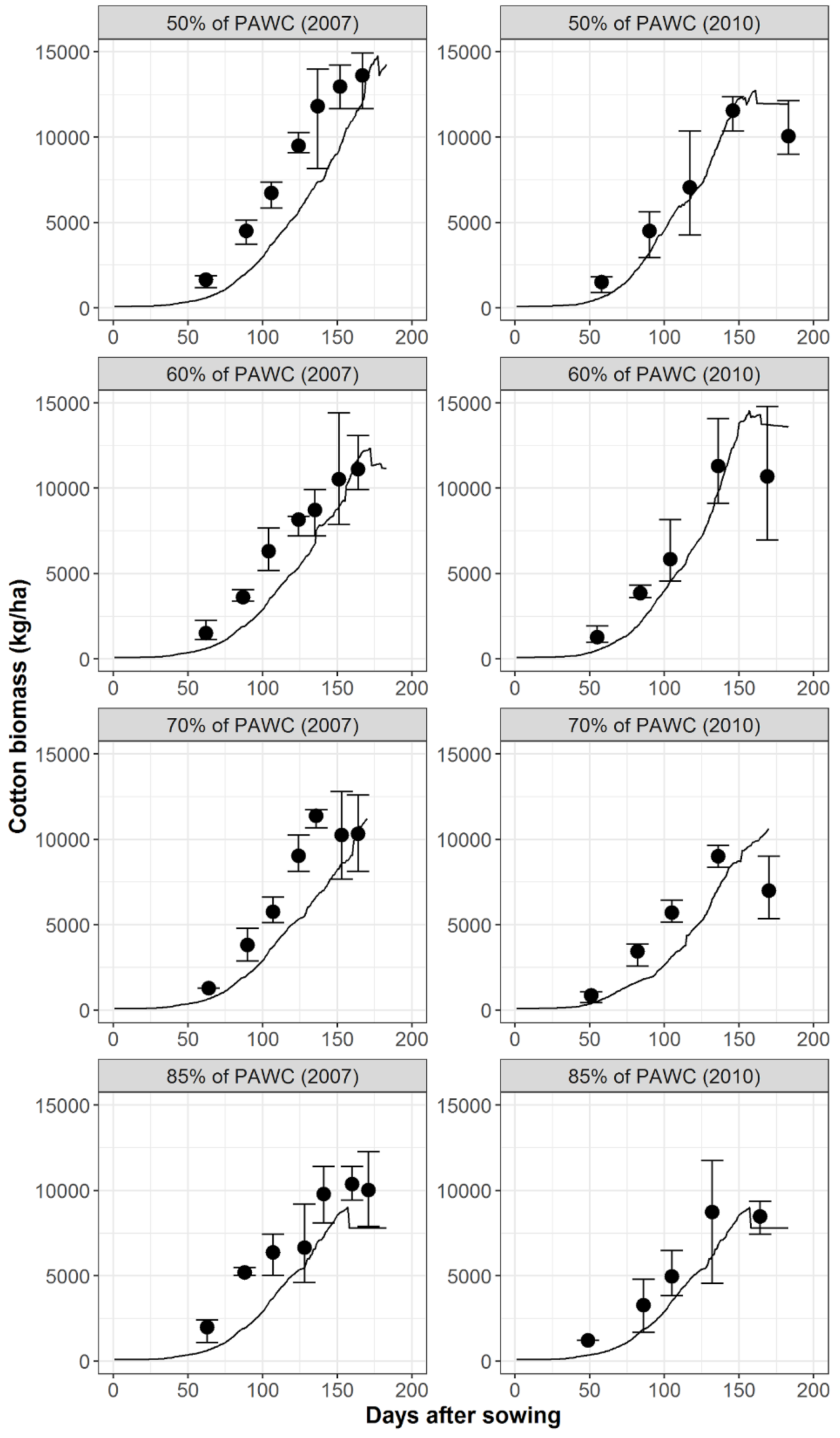
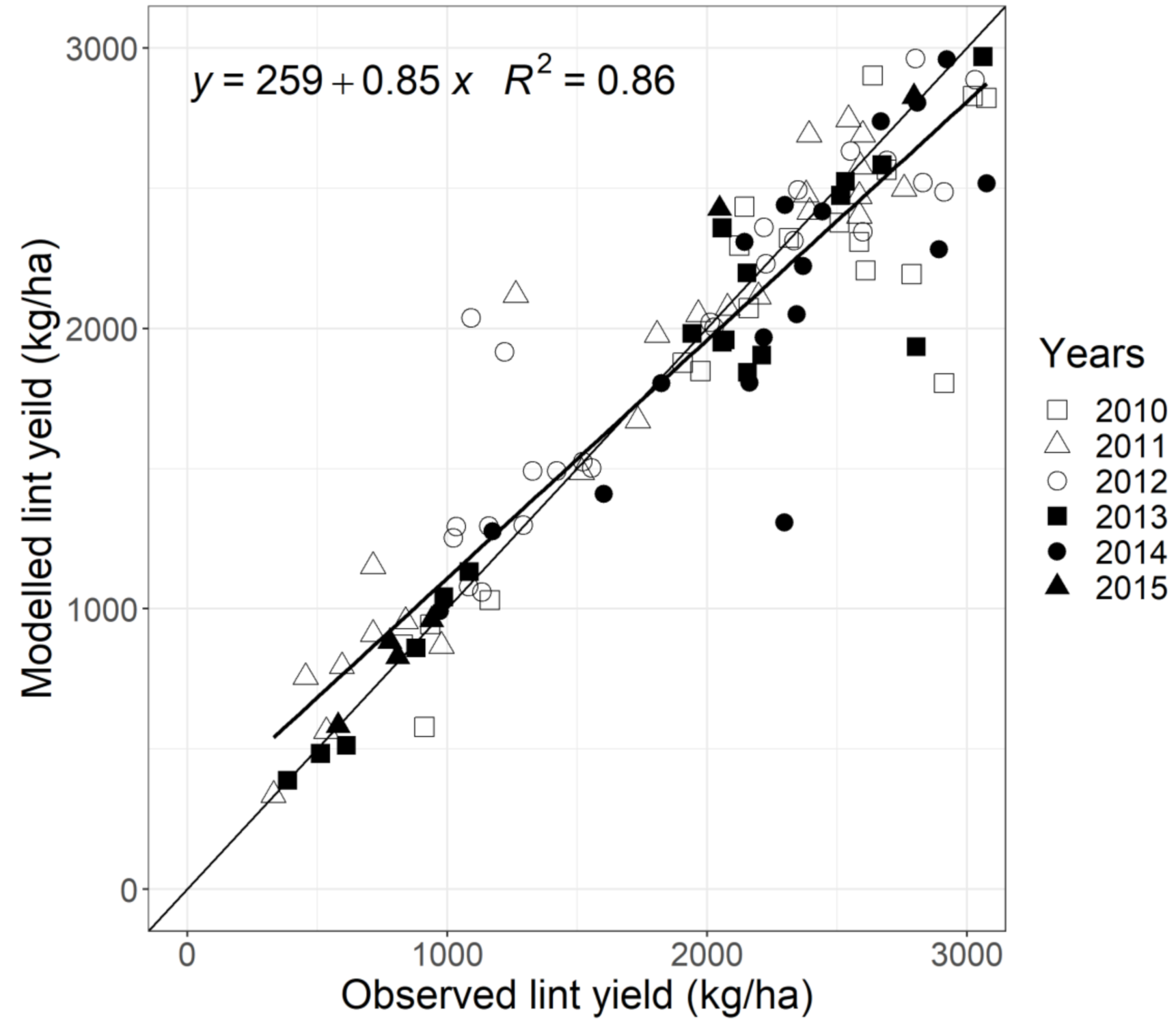
3.1. Model Validation

Validating the APSIM cotton model against biomass data given by Cammarano et al. [1] showed that the model was capable of predicting cotton biomass accumulation under a range of deficit irrigation practices (Figure 2). The summary statistics comparing modelled biomass to observed biomass were R2: 0.68, mean bias: 1476, model efficiency: 0.72, root mean square error: 2655, and concordance correlation coefficient: 0.82. Compared to observed biomass data, the APSIM model tended to underestimate crop biomass accumulation in both the 2007–2008 and 2009–2010 seasons. There was also a tendency to overestimate the final crop biomass (ca. 22%) in the 2009–2010 season, in which there were late season, heavy rainfall events (530 mm in total). These results demonstrate the model’s ability to produce an acceptable level of accuracy in the prediction of crop growth under a range of irrigation practices.
The APSIM model accurately predicted lint yield across the range of different environments, years, and crop management practices (Figure 3). The model slightly over-predicted yield in the lower yield potential simulations and slightly under-predicted lint yield in the higher yield potential simulations. The summary statistics comparing modelled yield to observed yield were R2: 0.86, mean bias: 32, model efficiency: 0.99, root mean square error: 280 and concordance correlation coefficient: 0.93. These summary statistics indicate that the model has an acceptable level of accuracy in representing cotton lint yield processes across a wide range of environments.

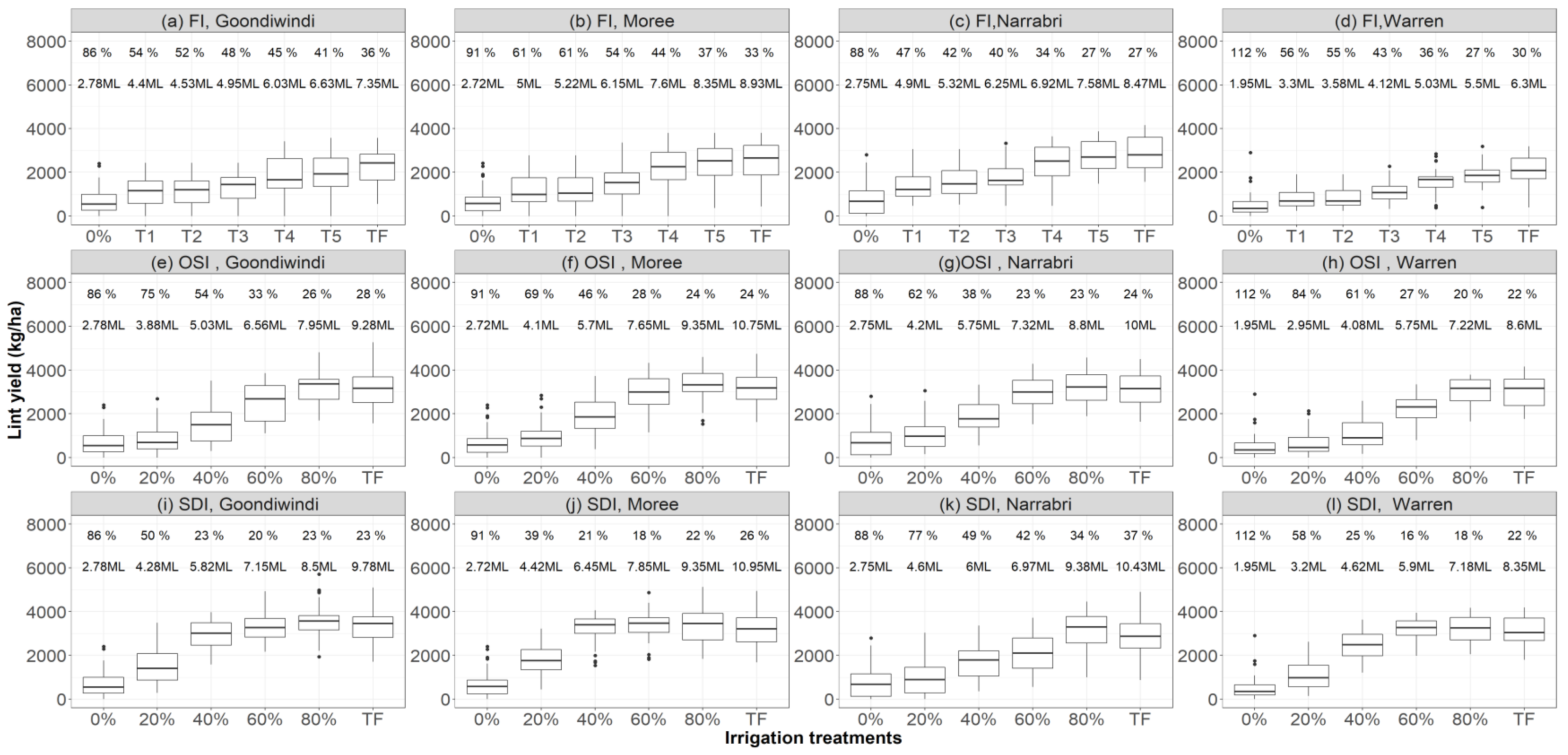
3.2. The Effects of Deficit Irrigation Practices on Lint Yield

For FI, the TF treatment achieved the greatest lint yield across all locations (Figure 4) indicating that for this irrigation system, where irrigation applications are infrequent, increasing water availability drives cotton yields. For this treatment, the median lint yields at Goondiwindi, Moree, Narrabri and Warren were 2427, 2667, 2800 and 2089 kg/ha, respectively; the average water applied was 7.35, 8.93, 8.47 and 6.30 ML/ha, respectively. As the amount of irrigation water applied increased, the CV of lint yield tended to decrease as the influence from rainfall variability decreased. The lowest CVs for Goondiwindi, Moree, Narrabri and Warren were 36% (for the TF treatment), 33% (TF), 27% (T5 and TF), and 27% (T5), respectively.
For the OSI system, across all study locations, the greatest median lint yield was achieved with 80% of TF treatment. This indicates that the practice of frequent applications of water, even at deficit levels, limits the exposure of the crop to yield limiting water deficits. For this treatment, the median lint yields at Goondiwindi, Moree, Narrabri and Warren were 3374, 3334, 3231 and 3179 kg/ha, respectively while the average water applied was 7.95, 9.35, 8.80 and 7.22 ML/ha, respectively. The 80% TF treatment saved, compared to the TF treatment, 1.33, 1.40, 1.20 and 1.38 ML/ha of water for Goondiwindi, Moree, Narrabri and Warren, respectively. As the amount of water applied increased under OSI, the CV of lint yield tended to decrease due to a reduced reliance on rainfall to meet water demands. The lowest CVs for Goondiwindi, Moree, Narrabri and Warren were 26% (at 80% of TF), 24% (at 80% of TF and TF), 23% (at 60% and 80% of TF) and 20% (at 80% of TF), respectively.
For the SDI system, the greatest median lint yield was achieved with the 80% of TF treatment at Goondiwindi and Narrabri, and 60% of TF treatment at Moree and Warren. This indicates that higher rainfall environments are able to compensate for the greater potential for exposure to water deficit with more restrictive DI practices applied with this irrigation system. For these treatments, the median lint yields at Goondiwindi, Moree, Narrabri, and Warren were 3568, 3470, 3296 and 3279 kg/ha, respectively; the average water applied was 8.50, 7.85, 9.38 and 5.90 ML/ha, respectively. The best performing treatments in terms of lint yield resulted in water savings of 1.28, 3.10, 1.03 and 2.45 ML/ha compared to the TF treatments for Goondiwindi, Moree, Narrabri and Warren, respectively. The lowest CVs for Goondiwindi, Moree, Narrabri and Warren were 20% (60% of TF), 18% (60% of TF), 34% (80% of TF) and 16% (60% of TF), respectively.

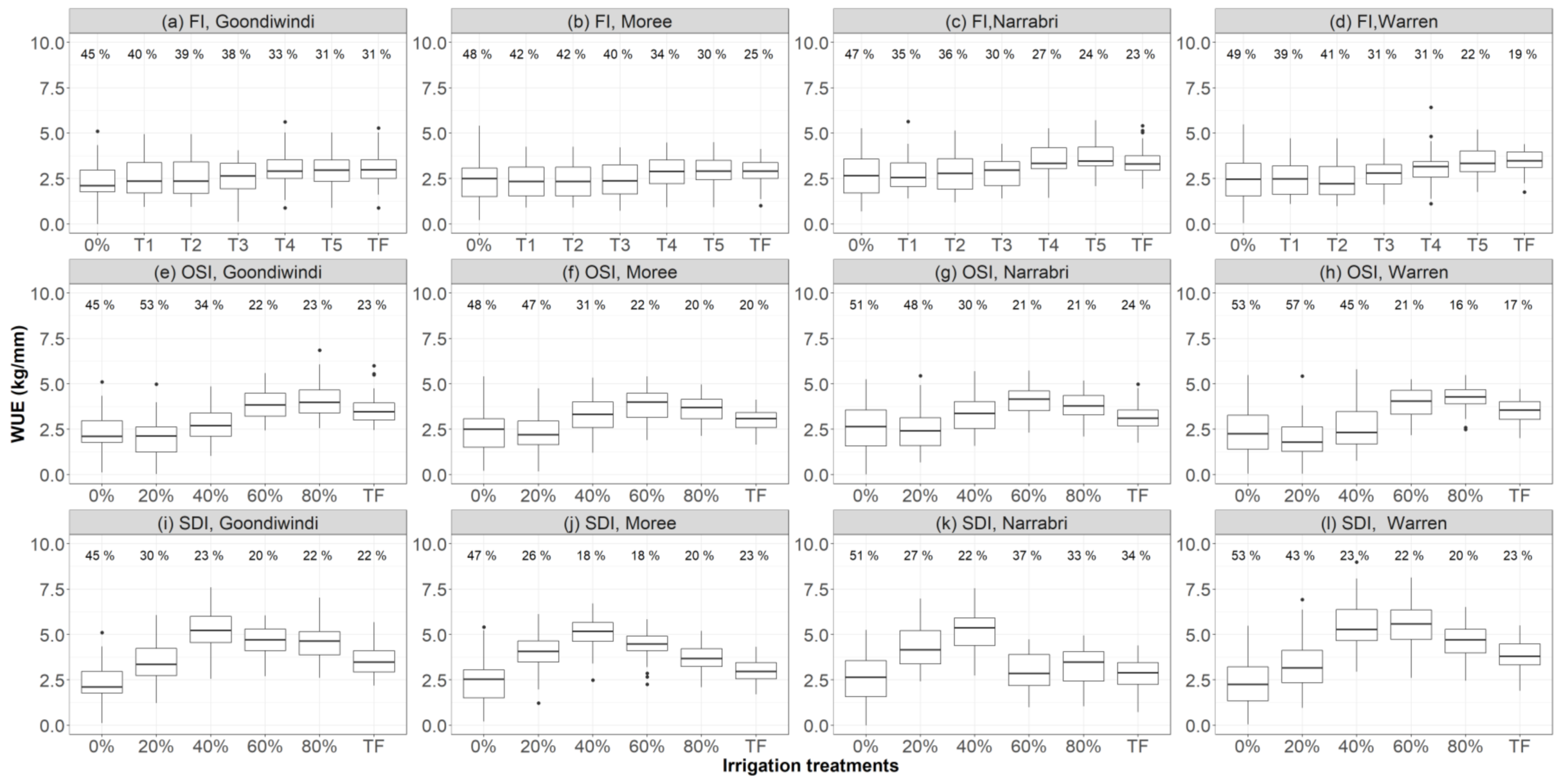
3.3. The Effects of Deficit Irrigation Practices on Water Use Efficiency

For the FI system, the greatest median WUE was achieved with the TF treatment at Goondiwindi, Moree and Warren, and T5 treatment at Narrabri (Figure 5) indicating the importance of limiting the exposure to water deficit stress on the agronomic performance of a FI system. For these treatments, the median WUE was 3.0, 2.9, 3.5, and 3.5 kg lint/mm, at Goondiwindi, Moree, Narrabri and Warren, respectively; the average total water applied was 7.34, 8.97, 7.57 and 6.42 ML/ha, respectively. As the amount of water applied increased, the CV of WUE tended to decrease as the influence of rainfall variability on the yield component of the WUE equation decreased. The lowest CVs for Goondiwindi, Moree, Narrabri and Warren were 31% (T5 and TF), 25% (TF), 23% (TF), and 19% (TF), respectively.
For the OSI system, the greatest median WUE was achieved with the 80% of TF treatment at Goondiwindi and Warren, and 60% of TF treatment at Moree and Narrabri. This was driven by a relatively greater decrease in the Tw component of the WUE equation compared to the yield component. For these treatments, the median WUEs at Goondiwindi, Moree, Narrabri and Warren were 4.0, 4.0, 4.2, and 4.3 kg lint/mm, respectively; the average total water applied was 7.69, 7.57, 7.37, and 7.21 ML/ha, respectively. The lowest CVs for Goondiwindi, Moree, Narrabri and Warren were 22% (60% of TF), 20% (80% of TF and TF), 21% (60% and 80% of TF), and 16% (80% of TF), respectively.
For the SDI system, the greatest median WUEs were achieved with 40% of TF treatment at Goondiwindi, Moree and Narrabri and 60% of TF treatment at Warren. For these treatments, the median WUEs at Goondiwindi, Moree, Narrabri, and Warren were 5.2, 5.2, 5.4 and 5.6 kg lint/mm, respectively; with the average total water applied 5.74, 6.47, 5.96 and 5.97 ML/ha, respectively. The lowest CVs for Goondiwindi, Moree, Narrabri and Warren were 20% (60% of TF), 18% (40% and 60% of TF), 22% (40% of TF), and 20% (80% of TF), respectively.

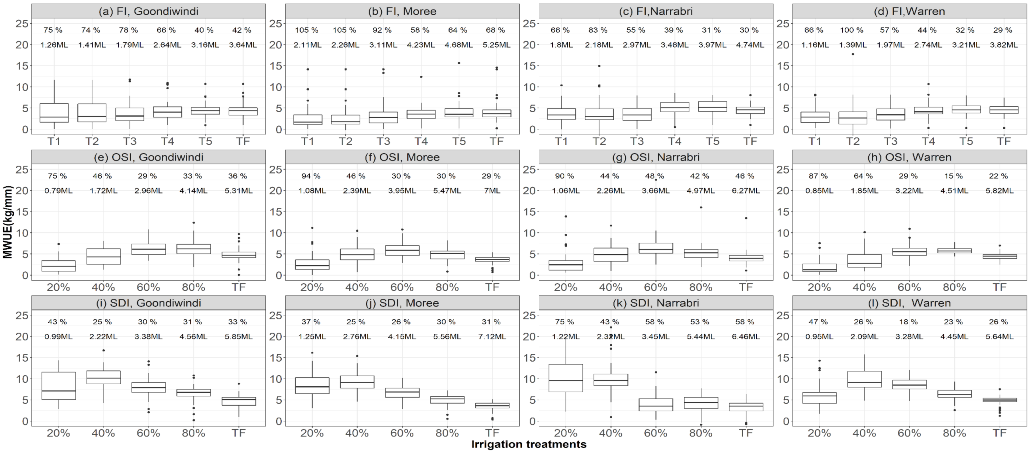
3.4. The Effects of Deficit Irrigation Practices on Marginal Water Use Efficiency

For the FI system, the greatest median MWUE was achieved with the T5 treatment at Goondiwindi and Narrabri, and the TF treatment at Moree and Warren (Figure 6) due to this system requiring large volumes of irrigation water to maximise its performance metrics. For these treatments, the median MWUEs at Goondiwindi, Moree, Narrabri and Warren were 4.5, 3.6, 5.2 and 4.6 kg lint/mm irrigation, respectively; and the average irrigation water applied was 3.16, 5.25, 3.97 and 3.82 ML/ha, respectively. As the amount of irrigation water increased, the CV of MWUEs tended to decrease as variance in the irrigated yields decreased. The lowest CV for Goondiwindi, Moree, Narrabri and Warren were 40% (T5), 58% (T4), 30% (TF), and 29% (TF), respectively.
For the OSI system, the greatest median MWUE was achieved with the 80% of TF treatment at Goondiwindi and Warren, and 60% of TF treatment at Moree and Narrabri due to the greater relative reduction in irrigation water applied compared the relative reduction in yield. For these treatments, the median MWUEs at Goondiwindi, Moree, Narrabri and Warren were 6.2, 5.9, 6.1, and 5.7 kg/mm, respectively. These values were achieved with an average irrigation water use of 4.14, 3.95, 3.66, and 4.51 ML/ha, respectively. The lowest CVs for MWUE at Goondiwindi, Moree, Narrabri and Warren were 29% (60% of TF), 29% (TF), 42% (80% of TF), and 15% (80% of TF), respectively.
For the SDI system, the greatest average MWUE was achieved with the 40% of TF treatment across all locations indicting that this system of the three investigated is potentially the best adapted to deficit irrigation practices. For this treatment, the median MWUEs at Goondiwindi, Moree, Narrabri, and Warren were 10.1, 9.1, 9.5 and 9.1 kg/mm, respectively; with an average irrigation water use of 2.22, 2.76, 2.32 and 2.09 ML/ha, respectively. The lowest CVs for Goondiwindi, Moree, Narrabri and Warren were 25% (at 40% of TF), 25% (at 40% of TF), 43% (at 40% of TF), and 18% (at 60% of TF), respectively.

4. Discussion

Before applying APSIM to model DI practices, we validated the model for its ability to model deficit irrigation (DI) through comparisons to observed crop biomass (Figure 2) and lint yield (Figure 3) from both experimental field data and industry production data across the MDB. We showed that the APSIM crop model was able to accurately predict crop biomass and lint yield. This is in alignment with previous reports. Carberry et al. [30] previously showed that the APSIM model accurately simulated a range of different crops, including cotton grown in Dalby, QLD., Australia. Earlier versions of the APSIM cotton model (APSIM-OZCOT) accurately predicted lint yield in two locations in Xinjiang, northwest China [27]. The robustness of the APSIM’s ability to represent croton growth and yield processes is testament to the suitability for modelling cotton crops and the impacts of management practices across the MDB. We, therefore, proceeded to use APSIM cotton to investigate the use of DI practices under three irrigation systems for four locations within the northern MDB.
Our results showed that modelled lint yield, WUE and MWUE under the FI system were lower than for the SDI (c.a. 27%, 8%, and 10% lower respectively for the TF treatment) and OSI (c.a. 25%, 8%, and 7% lower respectively for the TF treatment) systems (Figure 4, Figure 5 and Figure 6). This finding through modelling is supported by Lowien and Gall [17] who reported that field data from both OSI and SDI systems demonstrated greater yields (4% increase) and WUE (7% increase) compared to FI systems. Darouich et al. [16] also ascertained that irrigation by SDI systems produced approximately 42% higher lint yields than FI systems for the same amount of water used. Our modelling with APSIM suggests that the infrequent application of irrigations under FI systems results in periodic water deficit stress in the cotton crop, which reduces plant growth and leads to a reduction in lint yield.
Furthermore, our results indicated no beneficial effects of DI for FI systems in terms of lint yield. The findings of Wen [22] from field experiments in Southwest Texas, USA support our modelling in that there was no benefit for lint yield from DI practices under the FI system. However, there may be some small improvements in WUE and MWUE with DI under FI. In Goondiwindi and Narrabri, the T5 treatment led to the best outcomes for each of these measure (Figure 4, Figure 5 and Figure 6). There is likely an environmental influence on the suitability of deficit irrigation with a FI system with the practice potentially being better suited for environments with greater rainfall than those investigated in this study. Kaman et al. [48] reported that, when using DI in field experiments in Turkey, cotton yield was reduced, but WUE improved under a FI system. Their final conclusion aligns with our modelling results where the greatest lint yield will be achieved under a FI system using the TF treatment. This result is also supported by other researchers [48,49,50]. We conclude that the application of DI practices within a FI system results in lower lint yield because of crop stress due to the periodic wet and drying cycles. For the FI system, the results do not support our hypothesis that DI practices do not decrease lint yield in the MDB. However, in some higher rainfall situations, our hypotheses that DI achieved improvements with FI in terms of WUE and MWUE, is supported.
Some deficit irrigation practices had positive effects on predicted lint yield, WUE, and MWUE under the OSI system as the impact on yield was either positive or when negative was relatively minor compared to the reduction in Tw and WI. Our results indicated that, under an OSI system, lint yields, WUE and MWUE were all optimised with either 60% or 80% of the TF treatments (Figure 4, Figure 5 and Figure 6). The 80% of TF treatment compared to the TF treatment, saved between 1.20 and 1.40 ML/ha of irrigation water across the four study locations with minimal negative impact on yield. Study location had an effect on the actual optimisation point. Evans and Sadler [51] reported that both yield and WUE increased significantly when using deficit irrigation practices under an OSI system. Our modelling with APSIM and field observations by Evans and Sadler [51] support our hypothesis that, under an OSI system, the use of DI practices can increase lint yields, WUE and MWUE.
For the SDI system, DI practices had a positive effect on lint yield, WUE, and MWUE for all study locations, but there is some variation in the best DI treatment amongst locations. These differences may be dues to variation in average annual precipitation rates, especially lower summer rainfalls at Goondiwindi and Warren. Our results show that, under an SDI system, lint yields will be maximised by the use of 60% to 80% of the TF treatment DI practice. However, WUE and MWUE will be optimised with more restrictive applications of water, around 40% or 60% of TF (Figure 4, Figure 5 and Figure 6). The 40% of TF treatment compared to the TF treatment, saved between 2.09 and 2.76 ML/ha of irrigation water across the four study locations indicating a potential for DI practices to reduce water use when applied with an SDI system. The difference between the treatments that optimised yield and the treatments that maximised WUE and MWUE for the SDI system but not for the OSI and FI system suggests that there are system design aspects that demine if it is possible to optimise both yield and efficiency metrics through DI practices. Field experiments investigating DI for cotton grown with SDI systems identified that 80% of TF treatment achieved the greatest cotton yield [52]. Our modelling with APSIM and the findings of Sampathkumar et al. [52] from field research support our hypothesis that, under SDI system, the use of DI can increase lint yields and improve both WUE and MWUE by applying the optimum application of water.
Our results also demonstrate the effect of irrigation system choice on overall yields, WUE and MWUE. Yields, WUE and MWUE under the FI system with full irrigation were lower than yields under the OSI or SDI treatments with equivalent volumes of water application. Clearly, the increasing the utilisation OSI and DSI irrigation systems across the industry will lead to increased yields and improved WUE. This presents a significant opportunity to improve the productivity and WUE of the cotton industry, as 80% of cotton production occurs under furrow irrigation [4,12,13,14,15].
While this paper has investigated DI practices from a yield, WUE and MWUE perspective, financial returns will be a key driver of adopting DI practices on farms. If costs associated with purchasing and delivery of water are low, then a practice of applying 80% of TF treatment should be the most financially beneficial practice under OSI and SDI systems, excluding the initial start-up/capital costs which need to be further examined. However, if water is limited, costly and/or pumping costs are high, then a practice of applying 60% of TF might be the most financially beneficial practice for these systems. Alternatively, water saved could be used to irrigate more land, which would increase total cotton production and potentially whole farm financial returns.

5. Conclusions

Differences in lint yield and WUE, induced by the use of DI practices under three irrigation systems of FI, OSI and FI have been modelled with APSIM across four Australian cotton growing locations, using the APSIM cotton model. Our results showed that FI systems result in lower yields, WUE and MWUE than both OSI and SDI systems in all locations; moreover, DI is only a useful strategy for OSI and SDI systems to further improve these efficiency indicators. Therefore, growers should consider adoption OSI or SDI with DI practices. These results suggest it might be possible to grow more cotton with the same amount of water and increase WUE, with the use of DI practices and OSI and SDI systems. In terms of CV, the optimal DI practices resulted in lower yield variation for these two systems across all locations suggesting that DI practices may also reduce inter-annual yield variance. Water saving may be realised as reduced water consumption for a given level of lint production, or it may allow growers to increase the irrigated area, potentially increasing total cotton yields. However, given the overwhelming existing FI infrastructure across the industry, consideration of start-up/capital replacement costs and other costs should be considered in future research.

Author Contributions

H.H.S. contributed to conceptualisation, methodology, investigation, formal analysis, validation, writing and reviewing the original draft. K.G.P. contributed to conceptualisation, data analysis, writing and reviewing the original draft and provided supervision. A.F.Z. provided supervision and contributed to writing and reviewing the original draft. G.J.C. provided supervision and contributed to writing and reviewing the original draft. All authors have read and agreed to the published version of the manuscript.

Funding

This research received no external funding.

Institutional Review Board Statement

Not applicable.

Informed Consent Statement

Not applicable.

Data Availability Statement

Data sharing not applicable.

Acknowledgments

The authors are grateful to the former Executive Director of the University of Southern Queensland’s Institute for Life Sciences and the Environment, the late Steven Raine, for his advice around irrigation management of cotton crops. The authors thank King for her statistical advice and Harmes for her helpful comments on this manuscript. The first author’s PhD stipend was funded by the Ministry of Higher Education and Scientific Research, from the Government of Iraq.

Conflicts of Interest

H.H. Shukr, A.F. Zull and G.J. Cockfield declare no conflict of interest. K.G. Pembleton is an Editorial Board Member for Agronomy. Despite this relationship, he did not at any stage have editor-level access to this manuscript while in peer review.

References

  1. Cammarano, D.; Payero, J.; Basso, B.B.; Wilkens, P.; Grace, P. Agronomic and economic evaluation of irrigation strategies on cotton lint yield in Australia. Crop. Pasture Sci. 2012, 63, 647–655. [Google Scholar] [CrossRef]
  2. Stiller, W.N.; Wilson, I. Australian Cotton Germplasm Resources. In World Cotton Germplasm Resources; IntechOpen: London, UK, 2014; pp. 1–34. [Google Scholar]
  3. Azad, M.; Ancev, T. Economics of salinity effects from irrigated cotton: An efficiency analysis. Water Econ. Policy 2016, 2, 24. [Google Scholar] [CrossRef]
  4. Roth, G.; Harris, G.; Gillies, M.; Montgomery, J.; Wigginton, D. Water-use efficiency and productivity trends in Australian irrigated cotton: A review. Crop. Pasture Sci. 2013, 64, 1033–1048. [Google Scholar] [CrossRef] [Green Version]
  5. Seidl, C.; Wheeler, S.A.; Zuo, A. High turbidity: Water valuation and accounting in the Murray-Darling Basin. Agric. Water Manag. 2020, 230, 105929. [Google Scholar] [CrossRef]
  6. Wheeler, S.A.; Xu, Y.; Zuo, A. Modelling the climate, water and socio-economic drivers of farmer exit in the Murray-Darling Basin. Clim. Chang. 2019, 158, 551–574. [Google Scholar] [CrossRef]
  7. Perry, C.; Barnes, E.; Munk, D.; Fisher, K.; Bauer, P. Cotton Irrigation Management for Humid Regions; Cotton Incorporated: Cary, NC, USA, 2012. [Google Scholar]
  8. Qureshi, M.E.; Whitten, S.; Franklin, B. Impacts of climate variability on the irrigation sector in the southern Murray-Darling Basin, Australia. Water Resour. Econ. 2013, 4, 52–68. [Google Scholar] [CrossRef]
  9. Kodur, S.; Robinson, J.B. Modelling deep drainage rates of irrigation strategies under cropping sequence in subhumid, subtropical australia. Irrig. Drain. 2013, 63, 365–372. [Google Scholar] [CrossRef]
  10. An-Vo, D.-A.; Mushtaq, S.; Reardon-Smith, K.; Kouadio, L.; Attard, S.; Cobon, D.; Stone, R. Value of seasonal forecasting for sugarcane farm irrigation planning. Eur. J. Agron. 2019, 104, 37–48. [Google Scholar] [CrossRef]
  11. Qureshi, M.; Whitten, S. Regional impact of climate variability and adaptation options in the southern Murray–Darling Basin, Australia. Water Resour. Econ. 2014, 5, 67–84. [Google Scholar] [CrossRef]
  12. Brouwer, C.; Prins, K.; Kay, M.; Heibloem, M. Irrigation water management: Irrigation methods. Train. Man. 1988, 9, 5–7. [Google Scholar]
  13. Foley, J.P.; Raine, S.R. Overhead irrigation in the Australian cotton industry. Aust. Cottongrower 2002, 23, 40–44. [Google Scholar]
  14. Koech, R.K.; Smith, R.J.; Gillies, M. A real-time optimisation system for automation of furrow irrigation. Irrig. Sci. 2014, 32, 319–327. [Google Scholar] [CrossRef]
  15. Uddin, M.J.; Smith, R.J.; Gillies, M.H.; Moller, P.; Robson, D. Smart Automated Furrow Irrigation of Cotton. J. Irrig. Drain. Eng. 2018, 144, 04018005. [Google Scholar] [CrossRef] [Green Version]
  16. Darouich, H.; Pedras, C.G.; Gonçalves, J.M.; Pereira, L.S. Drip vs. surface irrigation: A comparison focussing on water saving and economic returns using multicriteria analysis applied to cotton. Biosyst. Eng. 2014, 122, 74–90. [Google Scholar] [CrossRef]
  17. Lowien, Z.; Gall, L. Grower Led Irrigation System Comparison in the Gwydir Valley. In CRDC1606 Technical Research Report; Gwydir Valley Irrigators Association Inc.: Moree, Australia, 2016. [Google Scholar]
  18. Dağdelen, N.; Başal, H.; Yılmaz, E.; Gürbüz, T.; Akçay, S. Different drip irrigation regimes affect cotton yield, water use efficiency and fiber quality in western Turkey. Agric. Water Manag. 2009, 96, 111–120. [Google Scholar] [CrossRef]
  19. Chai, Q.; Gan, Y.; Zhao, C.; Xu, H.-L.; Waskom, R.M.; Niu, Y.; Siddique, K.H.M. Regulated deficit irrigation for crop production under drought stress. A review. Agron. Sustain. Dev. 2016, 36, 1–21. [Google Scholar] [CrossRef] [Green Version]
  20. Capra, A.; Consoli, S.; Scicolone, B. Deficit irrigation: Theory and practice. Agric. Irrig. Res. Prog. 2008, 53–82. [Google Scholar]
  21. Mangalassery, S.; Rejani, R.; Singh, V.; Adiga, J.D.; Kalaivanan, D.; Rupa, T.R.; Philip, P.S. Impact of different irrigation regimes under varied planting density on growth, yield and economic return of cashew (Anacardium occidentale L.). Irrig. Sci. 2019, 37, 483–494. [Google Scholar] [CrossRef]
  22. Wen, Y. Spatial Variation of Soil Moisture and its Effect on Lint Yield in a Deficit Irrigated Cotton Field. bioRxiv 2017, 109025. [Google Scholar]
  23. Zhang, D.; Luo, Z.; Liu, S.; Li, W.; Tang, W.; Dong, H. Effects of deficit irrigation and plant density on the growth, yield and fiber quality of irrigated cotton. Field Crop. Res. 2016, 197, 1–9. [Google Scholar] [CrossRef]
  24. Kirda, C.; Moutonnet, P.; Hera, C.; Nielsen, D. Deficit Irrigation Practices. In Water Reports; FAO: Rome, Italy, 2002. [Google Scholar]
  25. Suleiman, A.A.; Soler, C.M.T.; Hoogenboom, G. Evaluation of FAO-56 crop coefficient procedures for deficit irrigation management of cotton in a humid climate. Agric. Water Manag. 2007, 91, 33–42. [Google Scholar] [CrossRef]
  26. Williams, A.; Mushtaq, S.; Kouadio, L.; Power, B.; Marcussen, T.; McRae, D.; Cockfield, G. An investigation of farm-scale adaptation options for cotton production in the face of future climate change and water allocation policies in southern Queensland, Australia. Agric. Water Manag. 2018, 196, 124–132. [Google Scholar] [CrossRef]
  27. Yang, Y.; Yang, Y.; Han, S.; Macadam, I.; Liu, D.L. Prediction of cotton yield and water demand under climate change and future adaptation measures. Agric. Water Manag. 2014, 144, 42–53. [Google Scholar] [CrossRef]
  28. Holzworth, D.P.; Huth, N.I.; Devoil, P.G.; Zurcher, E.J.; Herrmann, N.I.; McLean, G.; Chenu, K.; Van Oosterom, E.J.; Snow, V.; Murphy, C.; et al. APSIM—Evolution towards a new generation of agricultural systems simulation. Environ. Model. Softw. 2014, 62, 327–350. [Google Scholar] [CrossRef]
  29. Meier, E.A.; Lilley, J.M.; Kirkegaard, J.; Whish, J.; McBeath, T.M. Management practices that maximise gross margins in Australian canola (Brassica napus L.). Field Crop. Res. 2020, 252, 107803. [Google Scholar] [CrossRef]
  30. Carberry, P.S.; Hochman, Z.; Hunt, J.R.; Dalgliesh, N.P.; McCown, R.; Whish, J.P.M.; Robertson, M.; Foale, M.A.; Poulton, P.L.; Van Rees, H. Re-inventing model-based decision support with Australian dryland farmers. 3. Relevance of APSIM to commercial crops. Crop. Pasture Sci. 2009, 60, 1044–1056. [Google Scholar] [CrossRef] [Green Version]
  31. Liu, K.; Harrison, M.T.; Hunt, J.; Angessa, T.T.; Meinke, H.; Li, C.; Tian, X.; Zhou, M. Identifying optimal sowing and flowering periods for barley in Australia: A modelling approach. Agric. For. Meteorol. 2020, 282, 107871. [Google Scholar] [CrossRef]
  32. Hearn, A. OZCOT: A simulation model for cotton crop management. Agric. Syst. 1994, 44, 257–299. [Google Scholar] [CrossRef]
  33. CSD. Cotton Seed Distributors, Variety Trial Results (2009–2015). 2017. Available online: http://www.csd.net.au/resources (accessed on 5 November 2017).
  34. SILO. SILO Climate Data. 2017. Available online: https://legacy.longpaddock.qld.gov.au/silo/ (accessed on 15 November 2020).
  35. Tedeschi, L.O. Assessment of the adequacy of mathematical models. Agric. Syst. 2006, 89, 225–247. [Google Scholar] [CrossRef]
  36. Willmott, C.; Matsuura, K. Advantages of the mean absolute error (MAE) over the root mean square error (RMSE) in assessing average model performance. Clim. Res. 2005, 30, 79–82. [Google Scholar] [CrossRef]
  37. DAF. Cotton Production Growing Cotton: Varieties, Planting and Irrigation. 2018. Available online: https://www.daf.qld.gov.au/business-priorities/plants/field-crops-and-pastures/broadacre-field-crops/cotton/growing (accessed on 13 June 2018).
  38. Nguyen, L.T.T.; Osanai, Y.; Anderson, I.C.; Bange, M.P.; Braunack, M.; Tissue, D.T.; Singh, B.K. Impacts of waterlogging on soil nitrification and ammonia-oxidizing communities in farming system. Plant Soil 2018, 426, 299–311. [Google Scholar] [CrossRef]
  39. Luo, Q.; Bange, M.; Braunack, M.; Johnston, D. Effectiveness of agronomic practices in dealing with climate change impacts in the Australian cotton industry—A simulation study. Agric. Syst. 2016, 147, 1–9. [Google Scholar] [CrossRef]
  40. Luo, Q.; Bange, M.; Johnston, D.; Braunack, M. Cotton production in a changing climate. In Building Productive, Diverse and Sustainable Landscapes, Proceedings of the17th Australian Agronomy Conference, Hobart, Australia, 20–24 September 2015; Australian Society of Agronomy Inc.: Hobart, Australia, 2015. [Google Scholar]
  41. Conaty, W.C.; Johnston, D.B.; Thompson, A.J.; Liu, S.; Stiller, W.N.; Constable, G. Use of a managed stress environment in breeding cotton for a variable rainfall environment. Field Crop. Res. 2018, 221, 265–276. [Google Scholar] [CrossRef]
  42. CSD. Cotton & Wheat Gross Margin Analysis; Cotton Seed Distributiors: Wee Waa, Australia, 2008. [Google Scholar]
  43. Hulugalle, N.R.; McCorkell, B.; Heimoana, V.F.; Finlay, L.A. Soil properties under cotton-corn rotations in Australian cotton farms. J. Cotton Sci. 2016, 20, 294–298. [Google Scholar]
  44. Jeffrey, S.J.; Carter, J.O.; Moodie, K.B.; Beswick, A.R. Using spatial interpolation to construct a comprehensive archive of Australian climate data. Environ. Model. Softw. 2001, 16, 309–330. [Google Scholar] [CrossRef]
  45. Dalgliesh, N.; Wockner, G.; Peake, A. Delivering soil water information to growers and consultants. In Proceedings of the 13th Australian Agronomy Conference, Perth, WA, Australia, 10–14 September 2006. [Google Scholar]
  46. Bhattarai, S.P.; Midmore, D.J.; Pendergast, L. Yield, water-use efficiencies and root distribution of soybean, chickpea and pumpkin under different subsurface drip irrigation depths and oxygation treatments in vertisols. Irrig. Sci. 2008, 26, 439–450. [Google Scholar] [CrossRef]
  47. Abdi, H.; Salkind, N. Coefficient of Variation. Encycl. Res. Des. 2012, 1, 169–171. [Google Scholar] [CrossRef]
  48. Kaman, H.; Çetin, M.; Kirda, C. Soil salinity in a drip and furrow irrigated cotton field under influence of different deficit irrigation techniques. J. Adnan Menderes Univ. Agric. Fac. 2008, 6, 243–253. [Google Scholar]
  49. Geerts, S.; Raes, D. Deficit irrigation as an on-farm strategy to maximize crop water productivity in dry areas. Agric. Water Manag. 2009, 96, 1275–1284. [Google Scholar] [CrossRef] [Green Version]
  50. Fereres, E.; Soriano, M.A. Deficit irrigation for reducing agricultural water use. J. Exp. Bot. 2007, 58, 147–159. [Google Scholar] [CrossRef] [Green Version]
  51. Evans, R.G.; Sadler, E.J. Methods and technologies to improve efficiency of water use. Water Resour. Res. 2008, 44. [Google Scholar] [CrossRef]
  52. Sampathkumar, T.; Pandian, B.; Rangaswamy, M.; Manickasundaram, P.; Jeyakumar, P. Influence of deficit irrigation on growth, yield and yield parameters of cotton–maize cropping sequence. Agric. Water Manag. 2013, 130, 90–102. [Google Scholar] [CrossRef]
Figure 1. The location of cotton crops that were used to validate Agricultural Production System sIMulator (APSIM)-cotton for lint yield.
Agronomy 11 00231 g001
Figure 2. Observed cotton biomass (close dots) for cotton grown at Oakey in QLD. For the 2007–2008 and 2009–2010 seasons under four irrigation treatments [1] and modelled biomass from APSIM (solid line). Irrigation treatments occurred when soil moisture was depleted to 50% of plant available water capacity (50% of PAWC), 60% of PAWC, 70% of PAWC, and 85% of PAWC. Each point represents the mean with the range in observed values represented by the error bars.
Agronomy 11 00231 g002
Figure 3. Modelled lint yield (kg/ha) compared to observed lint yield [33] at 27 locations across northern NSW and QLD for crops harvested between 2010 and 2015.
Agronomy 11 00231 g003
Figure 4. Cotton lint yield (kg/ha) predicted using APSIM cotton model in response to irrigation treatments for furrow irrigation (FI), overhead sprinkler irrigation (OSI), and subsurface drip irrigation (SDI) for Goondiwindi (a,e,i), Moree (b,f,j), Narrabri (c,g,k), and Warren (d,h,l) for the period 1977 to 2017. Irrigation treatments for FI were dryland (0%) irrigation water, ‘1 out of 4’ (T1), ‘1 out of 3’ (T2), ‘1 out of 2’ (T3), ‘2 out of 3’ (T4), ‘3 out of 4’ (T5) irrigation events, and (TF) full irrigation treatment. The treatments of OSI and SDI systems were 0% (dryland), 20% of TF, 40% of TF, 60% of TF, 80% of TF, and full irrigation treatment (TF). The percentages represent the coefficient of variation (CV). The numbers represent total water applied (in-crop rainfall plus irrigation; ML/ha) for each treatment.
Agronomy 11 00231 g004
Figure 5. Water use efficiency (WUE; kg/mm) predicted using APSIM cotton model in response to irrigation treatments for furrow irrigation (FI), overhead sprinkler irrigation (OSI), and subsurface drip irrigation (SDI) for Goondiwindi (a,e,i), Moree (b,f,j), Narrabri (c,g,k), and Warren (d,h,l) for the period 1977 to 2017. Irrigation treatments for FI were dryland (0%) irrigation water, ‘1 out of 4’ (T1), ‘1 out of 3’ (T2), ‘1 out of 2’ (T3), ‘2 out of 3’ (T4), ‘3 out of 4’ (T5) irrigation events, and (TF) full irrigation treatment. The treatments of OSI and SDI systems were 0% (dryland), 20% of TF, 40% of TF, 60% of TF, 80% of TF, and full irrigation treatment (TF). The percentages represent the coefficient of variation (CV). The numbers represent total water (in-crop rainfall plus irrigation; ML/ha) for each treatment.
Agronomy 11 00231 g005
Figure 6. Marginal water use efficiency (MWUE; kg/mm) predicted using APSIM cotton model in response to irrigation treatments for furrow irrigation (FI), overhead sprinkler irrigation (OSI), and subsurface drip irrigation (SDI) for Goondiwindi (a,e,i), Moree (b,f,j), Narrabri (c,g,k), and Warren (d,h,l) for the period 1977 to 2017. Irrigation treatments for FI were ‘1 out of 4’ (T1), ‘1 out of 3’ (T2), ‘1 out of 2’ (T3), ‘2 out of 3’ (T4), ‘3 out of 4’ (T5) irrigation events, and (TF) full irrigation treatment. The treatments of OSI and SDI systems were 20% of TF, 40% of TF, 60% of TF, 80% of TF, and full irrigation treatment (TF). The percentages represent the coefficient of variation (CV). The numbers represent irrigation water applied (ML/ha) for each treatment.
Agronomy 11 00231 g006
Table 1. Summary of four different irrigation regimes applied at Oakey, QLD. in Australia over two cotton growing seasons 2007–2008 and 2009–2010. Irrigation applications occurred when soil moisture was depleted to 50% of plant available water capacity (50% of PAWC), 60% of PAWC, 70% of PAWC, and 85% of PAWC.
Treatments at:Total Irrigation Water AppliedNumber of Irrigation Applications
50% of PAWC228 mm6
60% of PAWC83 mm3
70% of PAWC82 mm2
85% of PAWC0 mm (no irrigated)0
Table 2. Summary of soil and climate details for each location used in the DI simulations. Soil water properties are drained upper limit, (DUL; mm); soil water capacity at 1500 kPa drained lower limit (DLL; mm); and plant available water capacity (PAWC; mm). Soil properties are the totals from the surface to 1.8 m soil depth and monthly climatic averages are for the 41 years from 1977 to 2017.
LocationsLat./Long.APSIM Soil NumberSoil TypeDULDLLPAWCAverage Annual RainfallTotal Annual EvaporationMaximum and Minimum Mean Monthly Temperatures (°C)
JanFebMarAprMayJunJulAugSepOctNovDec
Goondiwindi (QLD)−28.54° S/150.3 E219Clay vertisol4812802536142054323231272119192125283133
20211814106569141719
Moree
(NSW)
−29.48° S/149.83° E870Clay vertisol5623163725942178302131272219181924263133
2020171196559121619
Narrabri
(NSW)
−30.34° S/149.75° E125Clay vertisol6283502796522005312219182319162024273132
1912612864188121617
Warren
(NSW)
−31.78° S/147.76° E705Medium clay vertisol4542572344872038303330262117161822263032
1719161285447111517
Table 3. Deficit irrigation treatments (with the codes that they are referred to by subsequently in this manuscript) under the furrow irrigation (FI), overhead sprinkler irrigation (OSI) and sub-surface drip irrigation (SDI) systems across four locations. For FI, DI treatments were achieved by skipping one or more full irrigation (TF) irrigation events, e.g., T5 irrigates three out of four TF applications and skips one. For both OSI and SDI systems, DI treatments were achieved by applying a reduced amount of water on all occasions, e.g., 80% treatment applied 80% of TF water on all irrigations occasions.
Code FI TreatmentsCodeOSI and SDI Treatments
TFFull irrigation treatmentTFFull irrigation treatment
T1Irrigated 1 out of 4 TF irrigation events 20%Irrigated 20% of TF application
T2Irrigated 1 out of 3 TF irrigation events40% Irrigated 40% of TF application
T3Irrigated 1 out of 2 TF irrigation events60% Irrigated 60% of TF application
T4Irrigated 2 out of 3 TF irrigation events80% Irrigated 80% of TF application
T5Irrigated 3 out of 4 TF irrigation events
0%Dryland 0%Dryland
Publisher’s Note: MDPI stays neutral with regard to jurisdictional claims in published maps and institutional affiliations.

