Fused-Deep-Features Based Grape Leaf Disease Diagnosis

Abstract

Rapid and accurate grape leaf disease diagnosis is of great significance to its yield and quality of grape. In this paper, aiming at the identification of grape leaf diseases, a fast and accurate detection method based on fused deep features, extracted from a convolutional neural network (CNN), plus a support vector machine (SVM) is proposed. In the research, based on an open dataset, three types of state-of-the-art CNN networks, three kinds of deep feature fusion methods, seven species of deep feature layers, and a multi-class SVM classifier were studied. Firstly, images were resized to meet the input requirements of the CNN network; then, the deep features of the input images were extracted via the specific deep feature layer of the CNN network. Two kinds of deep features from different networks were then fused using different fusion methods to increase the effective classification feature information. Finally, a multi-class SVM classifier was trained with the fused deep features. The experimental results on the open dataset show that the fused deep features with any kind of fusion method can obtain a better classification performance than using a single type of deep feature. The direct concatenation of the Fc1000 deep feature extracted from ResNet50 and ResNet101 can achieve the best classification result compared with the other two fusion methods, and its F1 score is 99.81%. Furthermore, the SVM classifier trained using the proposed method can achieve a classification performance comparable to that of using the CNN model directly, but the training time is less than 1 s, which has an advantage over spending tens of minutes training a CNN model. The experimental results indicate that the method proposed in this paper can achieve fast and accurate identification of grape leaf diseases and meet the needs of actual agricultural production.

1. Introduction

Grape is one of the most favorite fruits in the world, which contains a variety of vitamins, carotenoids, and polyphenols which have numerous benefits for human health such as anti-cancer, anti-oxidation, and photoprotective [1,2]. Italy, France, Spain, the United States, and China are the main producers of grapes. According to the survey data of the Food and Agriculture Organization of the United Nations, grape disease is the main reason for the decrease in global grape production. However, most grape diseases start from the leaves and then spread to the entire plant. Therefore, a method which could identify grape leaf diseases with high accuracy will help to improve the management of grape production and provide a good growth environment.

Conventional expert diagnosis of grape leaf disease has the disadvantage of high cost and large risk of error. With the development of computer vision (CV), machine learning (ML), and deep learning (DL), technology has been widely applied to crop disease detection [3,4]. Conventional machine vision methods segment crop diseases spots using handcraft features such as color, texture, or shape. However, the characteristics of different diseases’ symptoms are highly similar. As a result, it is difficult to judge the types of diseases, and the accuracy of disease recognition is poor, especially in a complex natural environment. Compared to the conventional machine learning method, deep learning can often achieve better performance. A convolutional neural network (CNN) is a high-performance deep learning network which provides end-to-end pipelines to automatically learn the expressed hierarchical features hidden in the images [5,6,7]. Plant disease diagnosis based on deep networks is not only more effective but also avoids the tedious features selection procedure.

Nowadays, CNN-based models have been widely applied for early disease detection in crops and subsequent disease management. Atila et al. [8] adopted EfficientNet to realize plant disease diagnosis, with the help of transfer learning. A dataset with 38 categories of diseased leaves was used to train the networks. Finally, the highest accuracy of 99.97% was obtained on the B4 model. Long et al. [9] trained AlexNet and GoogleNet networks combined with a transfer learning strategy for Camellia oleifera diseases identification. Manpreet et al. [7] used a pre-trained ResNet network to classify 7 tomato diseases and an accuracy of 98.8% was achieved on the test dataset. A deep detection model structure for tomato leaf diseases was proposed by Karthik et al. [10]. The residual network was optimized and improved by the team to make it learn disease features more effectively. Yang et al. [11] used the saliency analysis of the image to locate pests in tea gardens. AlexNet was optimized using some tricks such as reducing the number of network layers and convolution kernels to improve the performance. The optimized model was effective against 23 pests in tea gardens, and an average recognition accuracy of 88.1% was obtained. In [12], a powerful neural network for identification of three different legume species based on the morphological patterns of the leaf veins was proposed by Grinblat et al. In summary, the above-mentioned literature provides a lot of references for the diagnosis of grape leaf disease in the real agriculture environment.

The above studies show that better performance can often be achieved by using a CNN network. However, a large dataset and huge computational resources are indispensable to train a deep network from scratch. Therefore, researchers began to study the method of combining deep features with support vector machines, that is, using CNN to extract deep features to train support vector machine classifiers to achieve fast, small-sample training of classifiers. In [13], deep features extracted by 13 CNN models (AlexNet, Vgg16, Vgg19, Xception, Resnet18, Resnet50, Resnet101, Inceptionv3, Inceptionresnetv2, GoogleNet, Densenet201, Mobilenetv2, shufflenet) were adopted to train an SVM classifier. The results show that the classifier trained by features extracted by Resnet50 is superior to other networks for rice disease recognition, and a F1 score of 0.9838 was obtained on the test dataset. In the same year, the method was adopted by the team to detect nitrogen deficiency of rice. The SVM classifier trained with ResNet50 deep features achieved the best performance with an accuracy of 99.84% [14]. In addition, an SVM classifier with the same idea as [13,14] was established by Jiang et al. [15] for rice leaf diseases diagnosis, and a mean correct identification accuracy of 96.8% was achieved.

The above research shows that using the deep features extracted using a CNN model to train the SVM classifier can obtain classification performance that is not inferior to those applying a deep network directly. In addition, compared with training a deep network from scratch, the computing resources and training time of training a support vector machine classifier are significantly reduced. The problem of the proposed deep features plus support vector machine classification method is that the current research is mainly focused on finding the best deep feature for classification, i.e., evaluating the performance of an SVM model trained using deep features of a specific layer of a single CNN model. There is no research on further processing the deep features extracted from different CNN networks to further improve the identification performance. To solve the above-mentioned problem in the current research, a method to train an SVM classifier with fused deep features is proposed to further improve the diagnosis performance of grape leaf disease. Compared with the single type of deep features, the fused deep features from different networks can make the SVM classifier learn more features and improve the classification performance. The main contributions of this study are as follows:

(1)

The deep features extracted by CNN models were adopted to train a support vector machine (SVM) classifier for the classification of grape leaf disease.

(2)

Three deep feature fusion methods were adopted to fuse deep features extracted from different CNN models to improve the classification performance of the classifier.

(3)

A comprehensive analysis of the deep feature plus SVM, fused deep features plus SVM, and conventional deep learning methods was carried out.

The rest of the paper is organized in the following manner. In Section 2, the studied dataset and the proposed method is given. Then, in Section 3, a comprehensive discussion based on the experiment results is presented. Finally, a conclusion of the research is given in Section 4.

2. Materials and Methods

2.1. Dataset

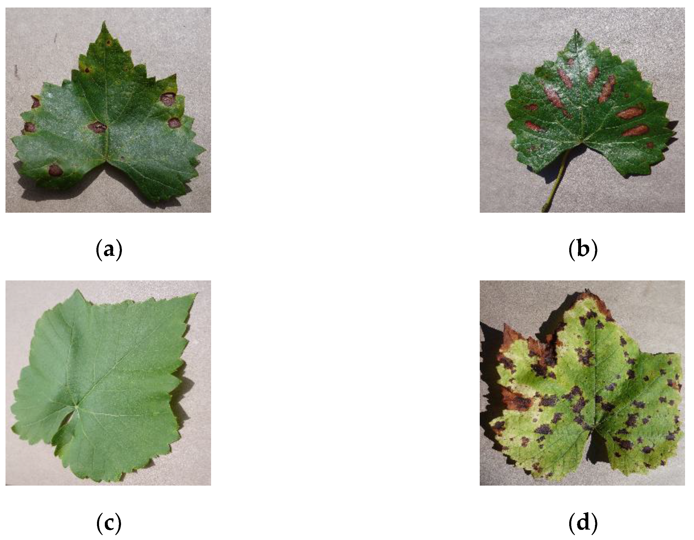
The dataset adopted to evaluate the performance in this study is a publicly available grape leaf disease dataset, which can be downloaded at http://www.kaggle.com (1 August 2021). The database of Kaggle, which is the largest database in the world, contains a large number of plant disease images. The dataset contains 4062 images (resolution: 256 × 256) with a total of 4 kinds of grape leaves (black rot, esca measles, leaf spot, and healthy). A detailed distribution of the dataset is shown in

Table 1. Grape leaf disease dataset.

Category	Amount
Black rot	1180
Esca measles	1383
Healthy	423
Leaf blight	1076
Total	4062

, and the images of grape leaves in 4 categories are shown in Figure 1.

2.2. Network Architecture and Deep Features Layers

In this study, the deep features extracted from three state-of-the-art CNN models, i.e., AlexNet [16], GoogLeNet [17], and ResNet [18], were adopted to evaluate the performance of the proposed method. All the deep features are extracted from a fully connected layer of a CNN model. Generally, a CNN network may contain several different fully connected layers (deep feature layers), e.g., the AlexNet has three fully connected layers of fc6, fc7, and fc8. Then, in this research, only some typical deep feature layers were examined, and detailed information of the selected layers is listed in

Table 2. The deep feature layer and feature vector of the studied CNN network.

CNN Models	Feature Layer	Feature Vector
AlexNet	fc6	4096
	fc7	4096
	fc8	1000
GoogLeNet	loss3-classifier	1000
ResNet18	Fc1000	1000
ResNet50	Fc1000	1000
ResNet101	Fc1000	1000

.

2.2.1. AlexNet

AlexNet was proposed by Alex Krizhevsky et al. [16]. and won first place in the ImageNet competition in 2012. The proposal of AlexNet is regarded as the beginning of deep learning. AlexNet, as shown in Figure 2, is a basic, simple, and effective CNN architecture, which is mainly composed of a convolutional layer, pooling layer, rectified linear unit (ReLU) layer, and fully connected layer. The success of AlexNet can be attributed to some practical strategies: (1) using ReLU nonlinear layers instead of a sigmoid function as activation functions, which can significantly accelerate the training phase and prevent overfitting; (2) a dropout strategy, which can be considered as a regularization to reduce the co-adaptation of neurons by setting the number of input neurons or hidden neurons to zero at random, was adopted to suppress overfitting; (3) the network was trained using multi-GPU to speed up the training phase. In this research, the deep features of fc6, fc7, and fc8 of AlexNet were examined.

2.2.2. GoogLeNet

GoogLeNetwas proposed by Christian Szegedy in 2014; before that, the deep learning networks obtained better performance by increasing the depth of the network (layers). However, with the increase of layers many problems, such as overfitting, gradient disappearance, and gradient explosion, may occur. In addition, when designing a network, only one operation such as convolution or pooling was used in a layer. Moreover, the size of the convolution kernel for the convolution operation is fixed. However, in practical situations, for different sizes of images, different sizes of convolution kernels are needed to produce the best performance, or for the same image, different sizes of convolution kernels behave differently because they have a different perceptual field. To address the above problems, GoogLeNet, constructed by Inception, was proposed. Inception puts multiple convolutions parallel together as a unit to form a network. Then, the model can choose the optimal convolutional kernels by adjusting the parameters during training. Networks constructed through inception modules can use computing resources more efficiently and can extract more features with the same amount of calculation. In this research, the deep feature layer of the loss3-classifier was examined.

2.2.3. ResNet

The residual network (ResNet) was proposed by He et al. [18], which could solve the degradation problem via the introduction of a residual module. The problem of network degradation refers to the decline of network accuracy with the deepening of network layers. It is certain that the performance degradation is not caused by overfitting, in which situation the accuracy should be high enough. Theoretically, for the problem of “accuracy decreases as the network deepens”, the residual block provides two options, i.e., identity mapping and residual mapping, where identity mapping (usually called “shortcut connection”) and residual mapping correspond to the x and F(x), respectively. The output of a residual block is y = F(x) + x (do not consider nonlinear activation). In the training phase, when the network has reached the optimum state, even if the network deepens, the residual mapping will be pushed to 0, leaving only identity mapping; then, the network is kept in optimum state and the performance will not decrease.

As shown in Equation (1), when the dimensions of $x$ and $F\left(x\right)$ are different, a linear projection $W$ should be applied on $x$ such that the dimensions of x could match the dimensions of $F\left(x\right)$.

$$y=F\left(x,\left\{W_i\right\}\right)+W_{x}x.$$

(1)

In this article, three widely used ResNet architectures, i.e., ResNet18, ResNet50, and ResNet101, were chosen as the deep feature extraction network. In addition, the deep features extraction layers shown in Table 2 were examined.

2.3. Fusion of Deep Features by Canonical Correlation Analysis

In this research, the canonical correlation analysis (CCA) [19] algorithm was adopted to fuse two kinds of deep features extracted by different networks of different deep features layers into a single feature vector. The fused feature is more discriminative than any of the input feature vectors. Canonical correlation analysis (CCA) has been widely adopted to analyze associations between two sets of variables.

Suppose that two ways are adopted to extract the $P$ and $q$ dimensional deep features of each sample, and two matrices, $X\in R^{p\times n}$ and $Y\in R^{q\times n}$, are obtained respectively, where $n$ is the number of samples. Then, a total of $\left(p+q\right)$ dimensional features of each sample are extracted.

Let $S_{xx}=R^{p\times p}$ and $S_{yy}=R^{q\times q}$ denote the within-sets covariance matrices of $X$ and $Y$ and $S_{xy}=R^{p\times q}$ denote the between-set covariance matrix between $X$ and $Y$. The matrix $S$ shown below is the overall $\left(p+q\right)\times \left(p+q\right)$ covariance matrix, which contains all the information on associations between the pairs of deep features.

$$S=\left(\begin{array}{cc}\mathrm{cov}(x)& \mathrm{cov}(x,y)\\ \mathrm{cov}(y,x)& \mathrm{cov}(y)\end{array}\right)=\left(\begin{array}{cc}{S}_{xx}& S_{xy}\\ S_{yx}& S_{yy}\end{array}\right).$$

(2)

However, the correlation between these two sets of deep feature vectors may not follow a consistent pattern, and therefore, it is difficult to understand the relationship between these two sets of deep features from this matrix [20]. The aim of CCA is to find a linear transformation, $X^{*}=W_x^{T}X$ and $Y^{*}=W_y^{T}Y$, and to maximize the pair-wise correlation between the two datasets:

$$corr(X^{*},Y^{*})=\frac{\mathrm{cov}(X^{*},Y^{*})}{var(X^{*})\cdot var(Y^{*})},$$

(3)

where $corr\left(X^{*},Y^{*}\right)=W_x^T{S}_{xy}{W}_y$, $var\left(X^{*}\right)=W_x^T{S}_{xx}{W}_x$ and $var\left(Y^{*}\right)=W_y^T{S}_{yy}{W}_y$. The covariance between $X^{*}$ and $Y^{*}$ ($X^{*},Y^{*}\in R^{d\times n}$ are known as canonical variables) is maximized using the Lagrange multiplier method, and the constraint condition is $var\left(X^{*}\right)=var\left(Y^{*}\right)=1$. Further, the linear transformation matrix $W_x$ and $W_y$ can be obtained by solving the eigenvalue equation as below [20]:

$$\{\begin{array}{c}{S}_{xx}^{-1}{S}_{xy}{S}_{yy}^{-1}{S}_{yx}{\widehat{W}}_x={\Lambda }^2{\widehat{W}}_x\\ S_{yy}^{-1}{S}_{yx}{S}_{xx}^{-1}{S}_{xy}{\widehat{W}}_y={\Lambda }^2{\widehat{W}}_y\end{array},$$

(4)

where ${\widehat{W}}_x$ and ${\widehat{W}}_y$ are the eigenvectors, and ${\Lambda }^2$ is a diagonal matrix of eigenvalues or squares of the canonical correlations.

The number of non-zero eigenvalues of each equation is $d=rank\left(S_{xy}\right)\le \min \left(n,p,q\right)$, further arranged in descending order, ${\lambda }_1\ge {\lambda }_2\ge \cdots \ge {\lambda }_d$. The transformation matrix $W_x$ and $W_y$ is composed of eigenvectors corresponding to sorted non-zero eigenvalues. For the transformed data, the form of the sample covariance matrix defined in Equation (2) is as follows:

$$S^{*}=\left(\begin{array}{cccccccc}1& 0& \cdots & 0& {\lambda }_1& 0& \cdots & 0\\ 0& 1& \cdots & 0& 0& {\lambda }_2& \cdots & 0\\ ⋮& & \ddots & & ⋮& & \ddots & \\ 0& 0& \cdots & 1& 0& 0& \cdots & {\lambda }_d\\ {\lambda }_1& 0& \cdots & 0& 1& 0& \cdots & 0\\ 0& {\lambda }_2& \cdots & 0& 0& 1& \cdots & 0\\ ⋮& & \ddots & & ⋮& & \ddots & \\ 0& 0& \cdots & {\lambda }_d& 0& 0& \cdots & 1\end{array}\right)$$

(5)

As shown in the above matrix, the upper left and lower right identity matrices indicate that the canonical variates are uncorrelated within each data set, and canonical variates have none zero correlation only on their corresponding indices.

As defined in [19], the deep features extracted by different CNN models could be fused via concatenation or summation of the transformed features (canonical variates $X^{*}$ and $Y^{*}$), and the fusion equations are shown in Equations (6) and (7).

$$Z_1=\left(\begin{array}{c}{X}^{*}\\ Y^{*}\end{array}\right)=\left(\begin{array}{c}{W}_x^{T}X\\ W_y^{T}Y\end{array}\right)={\left(\begin{array}{cc}{W}_x& 0\\ 0& W_y\end{array}\right)}^T\left(\begin{array}{c}X\\ Y\end{array}\right),$$

(6)

$$Z_2=X^{*}+Y^{*}=W_x^{T}X+W_y^{T}Y={\left(\begin{array}{c}{W}_x\\ W_y\end{array}\right)}^T\left(\begin{array}{c}X\\ Y\end{array}\right),$$

(7)

where $Z_1$ and $Z_2$ are named canonical correlation discriminant features (CCDFs). In this research, both the fusion methods shown in Equations (6) and (7) were adopted to achieve the fusion of deep features extracted from different CNN networks. In addition, the fusion method of a direct concatenation of two kinds of deep features extracted from different CNN networks was also evaluated in the experiment.

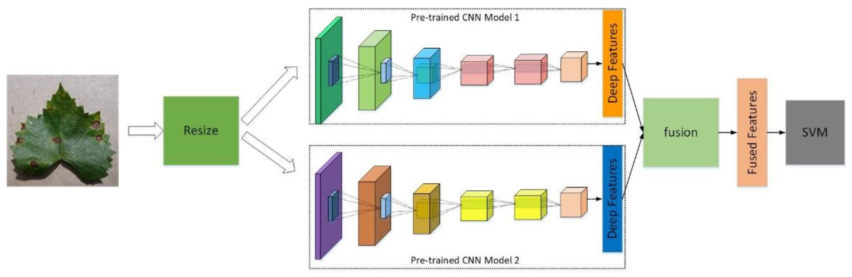
2.4. Proposed Methodology

The processing flow of the proposed method is demonstrated in Figure 3:

First, adjust the image size to make it fit the input requirement of the CNN models. The input requirements of the selected CNN models (AlexNet, ResNet, and GoogLeNet) are 227 × 227 × 3, 224 × 224 × 3, and 224 × 224 × 3, respectively.

Second, extract the deep features at specific layers of the CNN model. By inputting the image to the pre-trained CNN model and getting the parameter values on specified layers of the network, the specified deep feature can be obtained. The selected CNNs are pre-trained using ImageNet, which is a famous dataset for different applications. ImageNet contains more than 14 million images, covering more than 20,000 categories. As a result, more effective and meaningful deep features could be extracted by the pre-trained CNN models.

Third, make a fusion of the extracted deep features using one of the following methods, i.e., direct concatenation, canonical correlation analysis (CCA) concatenation, and canonical correlation analysis (CCA) sum.

Finally, feed the fused deep features into a fine-trained SVM classifier; then, the classifier can output the disease types of the input grape leaves. In the training stage, the “fit class error correcting output codes” (fitcecoc) function (MATLAB 2020b) with its default parameters was used, which can train a multi-class SVM classifier. The function of “fitcecoc” uses a K(K-1)/2 binary SVM model with a one-vs-one coding design, which enhances the classification performance of the classifier. Part of the default parameters adopted in the training stage are shown in

Table 3. Some typical parameters used in the training stage.

Parameter	Value
KernelFunction	linear
BoxConstraint	1
CacheSize	1000
OptimizeHyperparameters	none
IterationLimit	1e6

.

3. Experiment Result and Discussion

3.1. Experiment Setup

A Dell T7920 graphics workstation acted as the experiment platform. The basic configuration of the workstation is: Windows 10 operating system, two Intel Xeon Gold 6248R CPUs, two NVIDIA Quadro RTX 5000e GPUs, 64GRAM, and a 1T solid-state drive. The software environment is MATLAB 2020b, which can support some classical CNN models such as AlexNet, GoogLeNet, and ResNet by installing the DeepLearning toolbox. In addition, in the experiment, all the adopted CNN models (AlexNet, GoogLeNet, and ResNet) are pre-trained using ImageNet to ensure that they have powerful feature extraction capability.

3.2. The Evaluation Index

In the experiment, four metrics, i.e., accuracy, recall, precision, and F1 score, as shown in Equations (8)–(11), were adopted to evaluate the performance.

$$Accuracy=\frac{TP+TN}{TP+FP+TN+FN}$$

(8)

$$Recall=\frac{TP}{TP+FN}$$

(9)

$$Precision=\frac{TP}{TP+FP}$$

(10)

$$F1Score=2\times \frac{Precision\times Recall}{Precision+Recall}$$

(11)

where $TP$, $TN$, $FP$, and $FN$ represent the number of positive samples, true negative samples, false positive samples, and false negative samples.

3.3. Performance Analysis Based on Single Type of Deep Feature

The classification results of the fine-trained SVM classifier with a single type of deep feature are shown in

Table 4. Performance metrices and training time of SVM classifier with single deep feature (bold font shows the best performance).

Metrics (%)	AlexNet			GoogLeNet	ResNet18	ResNet50	ResNet101
	fc6	fc7	fc8	loss3-Classifier	Fc1000	Fc1000	Fc1000
Accuracy	98.60	97.32	95.94	96.75	97.76	99.08	98.86
Precision	98.88	97.85	96.67	97.35	98.19	99.26	99.08
Recall	98.88	97.80	96.57	97.23	98.16	99.24	98.95
F1 Score	98.88	97.82	96.62	97.29	98.17	99.25	99.01
Training time (S)	36.3458	1.0046	0.619	0.4914	0.4444	0.2596	0.3948

. In the experiment, in order to obtain more reliable experiment data, 10 independent runs for training and validation of each SVM classifier were made in the experiment, and their mean results were adopted to represent its performance. It was observed that, from Table 4, for the AlexNet network, the fc6 layer deep features have better performance compared with the other two kinds of deep layers. The Fc1000 layer of ResNet50 obtained the best classification performance compared with all the examined deep layers with accuracy, precision, recall, and F1 scores of 99.08%, 99.26%, 99.24%, and 99.25%, respectively. In addition, the training time of the SVM model with an fc6 layer of AlexNet takes the most time, with an average of 36.35 s, while the average time of all other single-type deep features was about 1 s or less. Because the fc6 layer of AlexNet can achieve better performance than fc7 and fc8, then, in the following sections, for the AlexNet network only the fc6 deep feature will be considered.

3.4. Performance Analysis Based on Fused Deep Features

3.4.1. Performance of Direct Concatenation Fusion Method

Table 5. Results of direct concatenation fusion method (bold font shows the best performance).

Fused Features	Accuracy (%)	Precision (%)	Recall (%)	F1 Score (%)	Dimension of the Fused Features
Alexnet + GoogLeNet	99.39	99.51	99.52	99.51	5096
Alexnet + ResNet 18	99.39	99.51	99.52	99.51	5096
Alexnet + ResNet50	99.36	99.48	99.49	99.49	5096
Alexnet + ResNet101	99.34	99.47	99.47	99.47	5096
GoogLeNet + ResNet18	98.90	99.12	99.12	99.12	2000
GoogLeNet + ResNet50	99.47	99.59	99.57	99.58	2000
GoogLeNet + ResNet101	99.57	99.66	99.65	99.66	2000
ResNet18 + ResNet50	99.54	99.63	99.63	99.63	2000
ResNet18 + ResNet101	99.54	99.62	99.64	99.63	2000
ResNet50 + ResNet101	99.77	99.81	99.80	99.81	2000

shows the performance of the SVM classifier trained using direct concatenation fusion of two deep features extracted from different CNN networks on the test set. Similar to the previous section, 10 independent runs for training and validation of each SVM classifier were made in the experiment, and their mean results were adopted to represent its performance (the following sections will adopt the same experiment method). It can be observed that the combination of ResNet50 (Fc1000) and ResNet101 (Fc1000) can get the best classification performance, while GoogLeNet (loss3-classifier) and ResNet18 (Fc1000) obtained the worst performance. Their accuracy, precision, recall, and F1 scores are 99.77%, 99.81%, 99.80%, and 99.81% and 98.90%, 99.12%, 99.12%, and 99.12%, respectively.

3.4.2. Performance of CCA Sum Fusion Method

Table 6. Results of CCA sum fusion method (bold font shows the best performance).

Features Type	Accuracy (%)	Precision (%)	Recall (%)	F1 Score (%)	Dimension of the Fused Features
Alexnet + GoogLeNet	96.55	97.29	97.15	97.22	787
Alexnet + ResNet 18	97.42	97.92	97.89	97.90	512
Alexnet + ResNet50	98.44	98.76	98.71	98.73	999
Alexnet + ResNet101	98.55	98.84	98.71	98.78	999
GoogLeNet + ResNet18	98.76	99.05	98.98	99.01	512
GoogLeNet + ResNet50	99.19	99.35	99.35	99.35	787
GoogLeNet + ResNet101	99.06	99.26	99.24	99.25	787
ResNet18 + ResNet50	99.36	99.48	99.49	99.48	512
ResNet18 + ResNet101	99.42	99.54	99.54	99.54	512
ResNet50 + ResNet101	99.57	99.67	99.65	99.66	999

shows the performance of the SVM classifier trained using CCA sum fusion of two deep features extracted from different CNN networks on the test set. It can be observed that the combination of ResNet50 (Fc1000) and ResNet101 (Fc1000) can get the best classification performance, while fc6 of AlexNet and GoogLeNet (loss3-classifier) obtained the worst performance. Their accuracy, precision, recall, and F1 scores are 99.57%, 99.66%, 99.64%, and 99.65% and 96.55%, 97.29%, 97.15%, and 97.22%, respectively.

3.4.3. Performance of CCA Concatenation Fusion Method

Table 7. Results of CCA concatenation fusion method (bold font shows the best performance).

Features Type	Accuracy (%)	Precision (%)	Recall (%)	F1 Score (%)	Dimension of the Fused Features
Alexnet + GoogLeNet	96.50	97.21	971	97.17	1574
Alexnet + ResNet 18	96.83	97.48	97.38	97.43	1024
Alexnet + ResNet50	98.14	98.52	98.45	98.49	1998
Alexnet + ResNet101	98.50	98.81	98.77	98.79	1998
GoogLeNet + ResNet18	98.81	99.05	99.05	99.05	1024
GoogLeNet + ResNet50	98.96	99.19	99.14	99.17	1574
GoogLeNet + ResNet101	99.09	99.29	99.26	99.27	1574
ResNet18 + ResNet50	99.27	99.42	99.37	99.39	1024
ResNet18 + ResNet101	99.26	99.41	99.38	99.39	1024
ResNet50 + ResNet101	99.56	99.65	99.64	99.64	1998

shows the performance of the SVM classifier trained using CCA concatenation fusion of two deep features extracted from different CNN networks on the test set. It can be observed that the combination of ResNet50 and ResNet101 can get the best classification performance, while fc6 of AlexNet and GoogLeNet obtained the worst performance. Their accuracy, precision, recall, and F1 scores are 99.55%, 99.65%, 99.64%, and 99.64% and 96.50%, 97.21%, 97.13%, and 97.17%, respectively.

3.5. Performance Comparison between 3 Deep Feature Fusion Method and a Single Deep Feature

In order to examine the influence of fusion features on the classification performance of the SVM classifier, in the experiment, we compare the performance of the three fusion methods with the corresponding single deep feature before fusion. Because the calculation of the F1 score integrates precision and recall, as shown in Equation (11), then the F1 score was adopted to evaluate the performance differences, and the results are shown in Figure 4. Each row shown in Figure 4 is the performance of the former deep features (deep features that would be used to make a fusion), the latter deep features (another deep features which would be used to make a fusion with the former deep features), the CCA sum fusion features, the CCA concatenation fusion features, and the direct concatenation fusion feature, respectively. It can be observed that for the fused deep features which contain the fc6 feature, only direct concatenation fusion can improve the performance, while the uses of CCA-related fusion methods will reduce the F1 score. The last 6 groups show that for the deep feature extracted using other CNN models, no matter which fusion method is used, the classification performance is better than that of a single deep feature.

Table 8. The best performance comparison between single deep feature and different fusion method (bold font shows the best performance).

Deep Features Type	Deep Features	Accuracy	Precision	Recall	F1 Score	Fusion Time	Train Time
Single type	ResNet50	99.08	99.26	99.24	99.25	-	0.2596
Direct concatenation	ResNet50+ResNet101	99.77	99.81	99.81	99.81	0.0062	0.4358
CCA concatenation	ResNet50+ResNet101	99.57	99.66	99.64	99.65	0.5106	1.5882
CCA sum	ResNet50+ResNet101	99.55	99.65	99.64	99.64	0.5118	2.0246

shows the performance comparison of the best results obtained via different methods (single feature, direct concatenation fusion, CCA concatenation fusion, CCA sum fusion). It can be seen from the table that among the three fusion methods, the direct concatenation of deep features can obtain better results than the fusion method of CCA. In addition, the SVM classifier trained via any fused deep feature can achieve better classification results than via a single deep feature, which indicates the method proposed in this paper could improve the classification performance compared with the existing methods related to deep feature plus SVM. The best F1 score is obtained via the direct concatenation of deep features extracted from ResNet50 (Fc1000) and ResNet101 (Fc1000), which is 0.56% higher than using ResNet50 (Fc1000) alone (F1 Score 99.25%, the best performance with a single deep feature). Further, from the view of time consumption, the shortest training time consumed by a single feature is only 0.2596 s, and no additional feature fusion time is needed, but for all three feature fusion methods, the total time of feature fusion and SVM classifier training is within 3 s.

3.6. Performance Comparison with Using CNN Network Directly

Table 9. The training parameters for the examined CNN models.

Parameters	Value
solver	sgdm
MiniBatchSize	20
InitialLearnRate	1 × e(−3)
MaxEpochs	50
ExecutionEnvironment	multi-gpu

is the training parameters for the examined CNN models. The “sgdm” was selected as the solver, and the values of “MiniBatchSize”, “InitialLearnRate”, and “MaxEpochs” were 20, 1 × e(−3), and 50, respectively. Furthermore, due to the workstation having two GPUs, then, the parameter of “ExecutionEnvironment” was set as “multi-gpu” to speed up the training.

The performance comparison between the feature fusion method proposed in this article and using a CNN network directly is obtained in

Table 10. Performance comparison between the proposed method and using CNN network directly (bold font shows the best performance).

Method	F1 Score (%)	Train Time
AlexNet	98.16	2470
GoogLeNet	98.16	2530
ResNet18	99.41	3023
ResNet50	99.72	3243
ResNet101	99.74	3437
Fused deep features (proposed by this study)	99.81	0.4358

. On the one hand, from the perspective of classification performance, the proposed method can obtain a slightly better performance than using any kinds of CNN network directly. On the other hand, from the view of the training time, based on the experimental environment of this paper, it usually takes tens of minutes to train a CNN network, while the fused deep feature + SVM method only takes less than 1 s to complete training. Therefore, we believe that the method proposed in this paper has certain advantages compared with using CNN models directly, especially in terms of the training time.

3.7. Performance Comparison with Some Other Studies

Table 11. Some other studies on plant leaf disease diagnosis.

No.	Reference	Plant Type	Dataset	Method	Accuracy
1	Liu et al. [21] (2020)	Grape	Augment by GANs (the original dataset is the same as ours)	Xception network	98.7%
2	Xie et al. [22] (2020)	Grape	62,944 images	Faster R-CNN combined with SE block	99.47%
3	Ji et al. [23] (2020)	Grape	1619 images	UnitedModel	98.5%
4	Adeel et al. [24] (2019)	Grape	The same with ours	SVM with CCA fused color, LBP, and geometric feature	92%
5	Tang et al. [25] (2020)	Grape	The same with ours	Squeeze-and-excitation added into ShuffleNet V1 and V2	99.14%
6	Yebasse et al. [26] (2021)	Coffee	1560 Robusta coffee leaf images	ResNet as the backbone	98%
7	Zhang et al. [27] (2019)	Cucumber	35,000 cucumber leaf images	GPDCNN model designed by the authors	95.81%

shows some studies on the diagnosis of plant diseases in recent years. Among them, studies 1 to 5 were the diagnosis of grape leaf diseases, while 6–7 were related to the diagnosis of other crop leaf diseases. It can be observed that the accuracy achieved by the proposed method in this paper outperforms that of those studies. Study 1 adopted the same dataset as ours, but it applied a GANs model to preprocess the original dataset to generate sufficient grape leaf disease images with prominent lesions. The Xception network was adopted as the classifier, and an accuracy of 98.7% was obtained on the augmented dataset. In study 2, an attention mechanism module, i.e., a squeeze-and-excitation block, was embedded into the Faster R-CNN model to make it focus on the more effective features, and an accuracy of 99.47 was achieved. In study 3, a UnitedModel was proposed, in which two CNN models are combined in parallel. The features extracted by each CNN models are concatenated and continue to flow to the fully connected layer and softmax layer to realize leaf disease diagnosis. The combination of multiple CNNs enables the proposed model to extract complementary discriminative features. Therefore, the representative ability of UnitedModel has been enhanced. The idea of that study is similar to ours, which is to make use of more deep features to improve the performance. However, the evaluated dataset is too small, which can easily cause overfitting, and the conventional machine learning models such as SVM are more suitable for a small dataset, as shown in our research. In addition, research 4 uses the same dataset as ours and also uses CCA fused features to train an SVM classifier. However, the features fused by CCA are conventional manual features, such as color, geometrics, etc. As a result, only an accuracy of 92% is obtained.

Although the performance obtained from our research outperforms that of the studies listed in Table 11. Many of their innovations are still worth learning. The diagnosis performance could be improved in a variety of ways. (1) The distinguishing features of the images could be retained and the interference features removed to improve the performance. For example, study 1 generates a dataset that highlights key features via GANs, study 6 removes the background of coffee leaves via a u²net, and study 7 only retains the region of lesions. (2) A better classification model could be used. On the one hand, we could select the network which is more suitable for a specific task through experiment; on the other hand, we can improve the structure of the CNN model. As shown in Table 11, studies 2 and 5 adopt attention mechanism to increase the network’s attention to the key features. (3) The classification features could be optimized. When using conventional machine classifiers such as SVM, an algorithm such as CCA, GA could be used to generate more discriminative features.

4. Conclusions and Future Works

Considering the need for diagnosis of various diseases during grape growth, an SVM plus fused deep feature method was proposed to identify three common grape leaves diseases and healthy leaves. In this paper, aiming at the identification of grape leaf diseases, a fast and accurate detection method based on fused deep, which extracted from a convolutional neural network (CNN), plus a support vector machine (SVM) is proposed. In the research, based on an open dataset, three types of state-of-the-art CNN networks, seven species of deep feature layers, three features fusion methods, and a multi-class SVM classifier were studied.

When using one type of deep feature to train the SVM classifier, the Fc1000 deep features can achieve the best classification performance, and its accuracy, precision, recall, and F1 scores are 99.08%, 99.26%, 99.24%, and 99.25%, respectively. When the feature fusion method is adopted, the performance is usually better, and the classification performance of direct concatenation is better than that of the CCA correlation fusion method. The best classification performance is obtained from the direct fusion of Fc1000 features of Resnet50 and Resnet101. Its accuracy, precision, recall and F1 scores are 99.77%, 99.81%, 99.81%, and 99.81%, respectively. The performance improvement verified that the proposed method does make sense. Furthermore, compared with using the CNN network directly, the proposed algorithm can also achieve a better classification performance. Especially, from the perspective of training time, in the experimental environment of this study, it usually takes tens of minutes to train a CNN network, while training the SVM with fused deep features only takes less than one second, which shows an obvious advantage.

In the future, work will be focused on model deployment. Many studies have implemented their algorithm on the smartphone [28,29,30,31], which is more convenient for end-users to diagnose diseases in situ. Generally, there are two candidate solutions to implement the proposed method on smartphones: (1) make the algorithm proposed in this article into a library file and develop an APP base on it; (2) deploy the algorithm in a cloud server, and the smartphone is responsible for sending image to the cloud server and receiving diagnosis results. The first scheme can enable the application to be used in the non-network environment, but depends on the computational ability, while the latter method needs good network bandwidth. In addition, although the proposed method could be applied to the diagnosis of other plant diseases theoretically, its versatility and effectiveness need to be further verified on other datasets in the future.

References

1. Mohamed Ahmed, I.A.; Özcan, M.M.; Al Juhaimi, F.; Babiker, E.F.E.; Ghafoor, K.; Banjanin, T.; Osman, M.A.; Gassem, M.A.; Alqah, H.A. Chemical composition, bioactive compounds, mineral contents, and fatty acid composi-tion of pomace powder of different grape varieties. J. Food Process. Preserv. 2020, 44, e14539. [Google Scholar] [CrossRef]
2. Sellitto, V.M.; Zara, S.; Fracchetti, F.; Capozzi, V.; Nardi, T. Microbial Biocontrol as an Alternative to Synthetic Fungi-cides: Boundaries between Pre-and Postharvest Applications on Vegetables and Fruits. Fermentation 2021, 7, 60. [Google Scholar] [CrossRef]
3. Boulent, J.; Foucher, S.; Theau, J.; St-Charles, P.-L. Convolutional Neural Networks for the Automatic Identification of Plant Diseases. Front. Plant Sci. 2019, 10, 941. [Google Scholar] [CrossRef] [Green Version]
4. Ma, J.; Zheng, F.; Zhang, L.; Sun, Z. Disease recognition system for greenhouse cucumbers based on deep convolutional neural network. Trans. Chin. Soc. Agric. Eng. 2018, 34, 186–192. [Google Scholar]
5. Arya, S.; Singh, R. A Comparative Study of CNN and AlexNet for Detection of Disease in Potato and Mango leaf. In Proceedings of the 2019 International Conference on Issues and Challenges in Intelligent Computing Techniques (ICICT), Ghaziabad, India, 27–28 September 2019; pp. 1–6. [Google Scholar]
6. Chao, X.; Sun, G.; Zhao, H.; Li, M.; He, D. Identification of Apple Tree Leaf Diseases Based on Deep Learning Models. Symmetry 2020, 12, 1065. [Google Scholar] [CrossRef]
7. Kaur, M.; Bhatia, R. Development of an improved tomato leaf disease detection and classification method. In Proceedings of the 2019 IEEE Conference on Information and Communication Technology, Baghdad, Iraq, 15–16 April 2019; pp. 1–5. [Google Scholar]
8. Atila, Ü.; Uçar, M.; Akyol, K.; Uçar, E. Plant leaf disease classification using EfficientNet deep learning model. Ecol. Inform. 2021, 61, 101182. [Google Scholar] [CrossRef]
9. Long, M.; Ouyang, C.; Liu, H.; Fu, Q. Image recognition of Camellia oleifera diseases based on convolutional neural network & transfer learning. Trans. Chin. Soc. Agric. Eng. 2018, 34, 194–201. [Google Scholar]
10. Karthik, R.; Hariharan, M.; Anand, S.; Mathikshara, P.; Johnson, A.; Menaka, R. Attention embedded residual CNN for disease detection in tomato leaves. Appl. Soft Comput. 2020, 86, 105933. [Google Scholar]
11. Yang, G.; Bao, Y.; Liu, Z. Localization and recognition of pests in tea plantation based on image saliency analysis and convolutional neural network. Chin. Soc. Agric. Eng. 2017, 33, 156–162. [Google Scholar]
12. Grinblat, G.L.; Uzal, L.C.; Larese, M.G.; Granitto, P. Deep learning for plant identification using vein morphological patterns. Comput. Electron. Agric. 2016, 127, 418–424. [Google Scholar] [CrossRef] [Green Version]
13. Sethy, P.K.; Barpanda, N.K.; Rath, A.K.; Behera, S.K. Deep feature based rice leaf disease identification using support vector machine. Comput. Electron. Agric. 2020, 175, 105527. [Google Scholar] [CrossRef]
14. Sethy, P.K.; Barpanda, N.K.; Rath, A.K.; Behera, S.K. Nitrogen Deficiency Prediction of Rice Crop Based on Convolutional Neural Network. J. Ambient. Intell. Humaniz. Comput. 2020, 11, 5703–5711. [Google Scholar] [CrossRef]
15. Jiang, F.; Lu, Y.; Chen, Y.; Cai, D.; Li, G. Image recognition of four rice leaf diseases based on deep learning and support vector machine. Comput. Electron. Agric. 2020, 179, 105824. [Google Scholar] [CrossRef]
16. Krizhevsky, A.; Sutskever, I.; Hinton, G.E. ImageNet classification with deep convolutional neural networks. Adv. Neural. Inf. Process. Syst. 2012, 25, 1097–1105. [Google Scholar] [CrossRef]
17. Szegedy, C.; Liu, W.; Jia, Y.; Sermanet, P.; Reed, S.; Anguelov, D.; Erhan, D.; Vanhoucke, V.; Rabinovich, A. Going deeper with convolutions. In Proceedings of the IEEE Conference on Computer Vision and Pattern Recognition, Boston, MA, USA, 7–12 June 2015; pp. 1–9. [Google Scholar]
18. He, K.M.; Zhang, X.Y.; Ren, S.Q.; Sun, J. Deep Residual Learning for Image Recognition. In Proceedings of the IEEE Conference on Computer Vision and Pattern Recognition, Las Vegas, NV, USA, 27–30 June 2016; pp. 770–778. [Google Scholar]
19. Sun, Q.-S.; Zeng, S.-G.; Liu, Y.; Heng, P.-A.; Xia, D.-S. A new method of feature fusion and its application in image recognition. Pattern Recognit. 2005, 38, 2437–2448. [Google Scholar] [CrossRef]
20. Krzanowski, W. Principles of Multivariate Analysis; Oxford University Press: Oxford, UK, 2000; Volume 23. [Google Scholar]
21. Liu, B.; Tan, C.; Li, S.; He, J.; Wang, H. A Data Augmentation Method Based on Generative Adversarial Networks for Grape Leaf Disease Identification. IEEE Access 2020, 8, 102188–102198. [Google Scholar] [CrossRef]
22. Xie, X.; Ma, Y.; Liu, B.; He, J.; Li, S.; Wang, H. A Deep-Learning-Based Real-Time Detector for Grape Leaf Diseases Using Improved Convolutional Neural Networks. Front. Plant Sci. 2020, 11, 751. [Google Scholar] [CrossRef] [PubMed]
23. Ji, M.; Zhang, L.; Wu, Q. Automatic grape leaf diseases identification via UnitedModel based on multiple convolu-tional neural networks. Inf. Process. Agric. 2020, 7, 418–426. [Google Scholar]
24. Adeel, A.; Khan, M.A.; Sharif, M.; Azam, F.; Shah, J.H.; Umer, T.; Wan, S. Diagnosis and recognition of grape leaf diseases: An automated system based on a novel saliency approach and canonical correlation analysis based multiple features fusion. Sustain. Comput. Inform. Syst. 2019, 24, 100349. [Google Scholar] [CrossRef]
25. Tang, Z.; Yang, J.; Li, Z.; Qi, F. Grape disease image classification based on lightweight convolution neural networks and channelwise attention. Comput. Electron. Agric. 2020, 178, 105735. [Google Scholar] [CrossRef]
26. Yebasse, M.; Shimelis, B.; Warku, H.; Ko, J.; Cheoi, K. Coffee Disease Visualization and Classification. Plants 2021, 10, 1257. [Google Scholar] [CrossRef] [PubMed]
27. Zhang, S.; Zhang, S.; Zhang, C.; Wang, X.; Shi, Y. Cucumber leaf disease identification with global pooling dilated convolutional neural network. Comput. Electron. Agric. 2019, 162, 422–430. [Google Scholar] [CrossRef]
28. Lee, K.-C.; Wang, Y.-H.; Wei, W.-C.; Chiang, M.-H.; Dai, T.-E.; Pan, C.-C.; Chen, T.-Y.; Luo, S.-K.; Li, P.-K.; Chen, J.-K.; et al. An Optical Smartphone-Based Inspection Platform for Identification of Diseased Orchids. Biosensors 2021, 11, 363. [Google Scholar] [CrossRef] [PubMed]
29. Machado, B.B.; Orue, J.P.M.; Arruda, M.S.; Santos, C.V.; Sarath, D.S.; Gonçalves, W.; Silva, G.G.; Pistori, H.; Roel, A.R.; Rodrigues, J.F.J. BioLeaf: A professional mobile application to measure foliar damage caused by insect herbivory. Comput. Electron. Agric. 2016, 129, 44–55. [Google Scholar] [CrossRef] [Green Version]
30. Petrellis, N. A smart phone image processing application for plant disease diagnosis. In Proceedings of the 2017 6th International Conference on Modern Circuits and Systems Technologies (MOCAST), Thessaloniki, Greece, 4–6 May 2017; pp. 1–4. [Google Scholar]
31. Petrellis, N. Plant Disease Diagnosis for Smart Phone Applications with Extensible Set of Diseases. Appl. Sci. 2019, 9, 1952. [Google Scholar] [CrossRef] [Green Version]
Figure 1. Grape leaf dataset: (a) black rot, (b) esca measles, (c) healthy, (d) leaf blight.
Agronomy 11 02234 g001
Figure 2. The architecture of AlexNet.
Agronomy 11 02234 g002
Figure 3. The processing flow of the proposed method.
Agronomy 11 02234 g003
Figure 4. Performance comparison of single deep feature and fusion deep features.
Agronomy 11 02234 g004