Positive Mathematical Programming to Model Regional or Basin-Wide Implications of Producer Adoption of Practices Emerging from Plot-Based Research

Abstract

A method for calibrating models of agricultural production and resource use for policy analysis is proposed to leverage multidisciplinary agricultural research at the National Center for Alluvial Aquifer Research (NCAAR). An illustrative example for Sunflower County, MS, is presented to show how plot-level research can be extended to draw systemic region or basin wide implications. A hypothetical improvement in yields for dryland soybean varieties is incorporated into the model and shown to have a positive impact on aquifer outcomes and producer profits. The example illustrates that a change in one practice-crop combination can have system-wide impacts, as evidenced by the change in acreages for all crops and practices.

1. Introduction

The National Center for Alluvial Aquifer Research (NCAAR) was created to conduct research aimed at developing novel irrigation and agricultural water management technologies to improve water productivity, and decrease irrigation water withdrawal from and increase the groundwater recharge to the Mississippi River Valley Alluvial Aquifer (MRVAA) with the overall objective of ensuring sustainable agricultural water supplies in the Lower Mississippi River Basin (LMRB). The complexity of natural resource management in general, and groundwater resources in particular, requires multidisciplinary research efforts that are reflected in the diverse background of the NCAAR researchers, from natural to social scientists. The complexity of the problem and the composition of NCAAR is represented in the conceptual diagram for the proposed USDA Agricultural Research Service (ARS) project under National Program 211: Water Availability and Watershed Management which funds NCAAR (see Figure 1). The complexity of the NCAAR mission is magnified by the challenge that the region receives significant rainfall annually, but the timing does not coincide with crop production. The rainfall timing is paired with evolving land use, long-term irrigation practices which must change, and a wide range of socio-economic classes of producers who must all adopt new practices. This paper presents a methodology that can bridge the inter-disciplinary obstacles to translate plot and field-level research results to regional or basin-wide potential outcomes that incorporate implicit producer behavior with minimal data requirements: positive mathematical programming.

The Mississippi River Valley Alluvial Aquifer (MRVAA, see Figure 2) is the primary source of water for irrigation for the Lower Mississippi River Basin (LMRB) and is depleting at an unsustainable rate [1,2]. The increase in global population, the resulting growing demand for food, and the receding irrigated acreage in areas where aquifers are depleting require ever increasing levels of productivity from agricultural areas that are relatively rich in water resources, such as the LMRB [3,4]. NCAAR’s mission leverages multidisciplinary agricultural research to alleviate and ultimately contribute to solving the problem of a depleting MRVAA. Aligned with this mission is research at the experimental plot or field level that reduces crop water use without a significant impact on baseline yields, increases crop productivity for a baseline level of water use, or increases the capture of available water by allowing earlier planting to capture natural precipitation or developing infrastructure to capture irrigation or pluvial runoff for reuse. Plot and field-level research in this area show growing evidence that important water savings are achievable with relatively minor modifications to existing irrigation and agronomic practices in the Mid-South USA [2,3,5,6,7,8,9,10]. However, regional or basin-wide implications of the potential results of wide producer adoption of these practices have not been explored.

Positive mathematical programming (PMP) is a methodology widely used for agricultural economic policy analysis because it requires minimal data; it is capable of characterizing resource, environmental, or policy constraints; and models that employ it are consistent with economic production theory [11]. Basically, PMP uses the shadow prices of calibration constraints from a profit maximization linear program (LP) to specify (calibrate) a non-linear objective function such that observed activity levels are reproduced by the optimal solution of the new unconstrained programming problem [12,13]. The form of the unconstrained programming model can be subsequently modified to incorporate farming, environmental, resource, or policy conditions not explicitly modeled [13]. The calibration step avoids the problem of over-specialization of corner solutions in which all the acres are assigned to the most profitable crops [14]. The analysis proceeds by evaluating changes in optimal allocations induced by changes introduced in the variables or parameters of interest. Furthermore, in the case of groundwater, dynamic simulations that update the state of the aquifer and other constraining resources over time allow one to project the impacts of those changes in the future.

The PMP methodology is particularly useful when data on individual decision units are unavailable, insufficient, or inadequate for econometric analysis. The absence of observations over a wide range of prices requires the use of programming approaches to estimate the elasticities of the derived demand for water [15,16]. A growing body of work has employed PMP to study water use or aquifer depletion implications in a variety of settings. For example, Pulido-Velazquez et al. [17] calibrated a set of functions of marginal economic benefit for surface-groundwater use in a hydroeconomic model of a river basin in Spain. Clark [18] explored the impacts of high commodity price scenarios on irrigated crop production, groundwater application to irrigation, and aquifer outcomes in Western Kansas. Esteban and Albiac [19] used PMP to calibrate a model of groundwater management under three aquifer management scenarios that incorporate ecosystem damages from groundwater over-pumping. Employing a formulation similar to Clark [18], Garay-Armoa [14] assessed the impacts of two water conservation practices (water use restrictions and permanent conversions to dryland crops) on the Ogallala Aquifer and on producer welfare for a set of counties in Kansas. Most recently, Lambert et al. [20] explored the effects of climate change on crop choices and irrigation adoption among farmers in Tennessee’s watersheds.

A major criticism of the programming approach is that the pre-specified functions may not precisely represent the biological and physical processes of, for example, plant growth [15,16]. However, several studies have been able to address this issue by applying PMP iteratively in combination with separate crop growth and hydrological models. Aistrup et al. [21] applied the formulation to Groundwater Management District 3 (GMD3) in southwestern Kansas in which PMP is used with a plant growth model integrating water and land use patterns, changing climate, economic trends, and population dynamics. In California, MacEwan et al. [22] developed a modular hydroeconomic modeling approach integrating California’s C2VSim groundwater-surface water simulation model with the Statewide Agricultural Production (SWAP) economic model. In that formulation, MacEwan et al. [22] considered a milti-input constant elasticity of substitution (CES) production function and a calibrated crop demand function that increases the robustness and sophistication of the analysis. Similarly, PMP is the core of the Central Valley Production Model (CVPM), a “multi-regional model of irrigated agricultural production that can forecast changes in crop acres as a function of changes in the availability of water supplies,” presented by Dale et al. [23]. Finally, Qureshi et al. [13] developed a biophysical-economic mathematical model with PMP that calibrated against the observed multi-period land use data to evaluate the impacts of droughts and a set of policy options on agricultural production in the Murray-Darling Basin, Australia.

In the following sections we describe the PMP methodology and how it can help integrate multidisciplinary plot or field-level research to project likely aquifer and producer welfare outcomes. Then we present a case study to illustrate the methodology and conclude with a discussion of the implications.

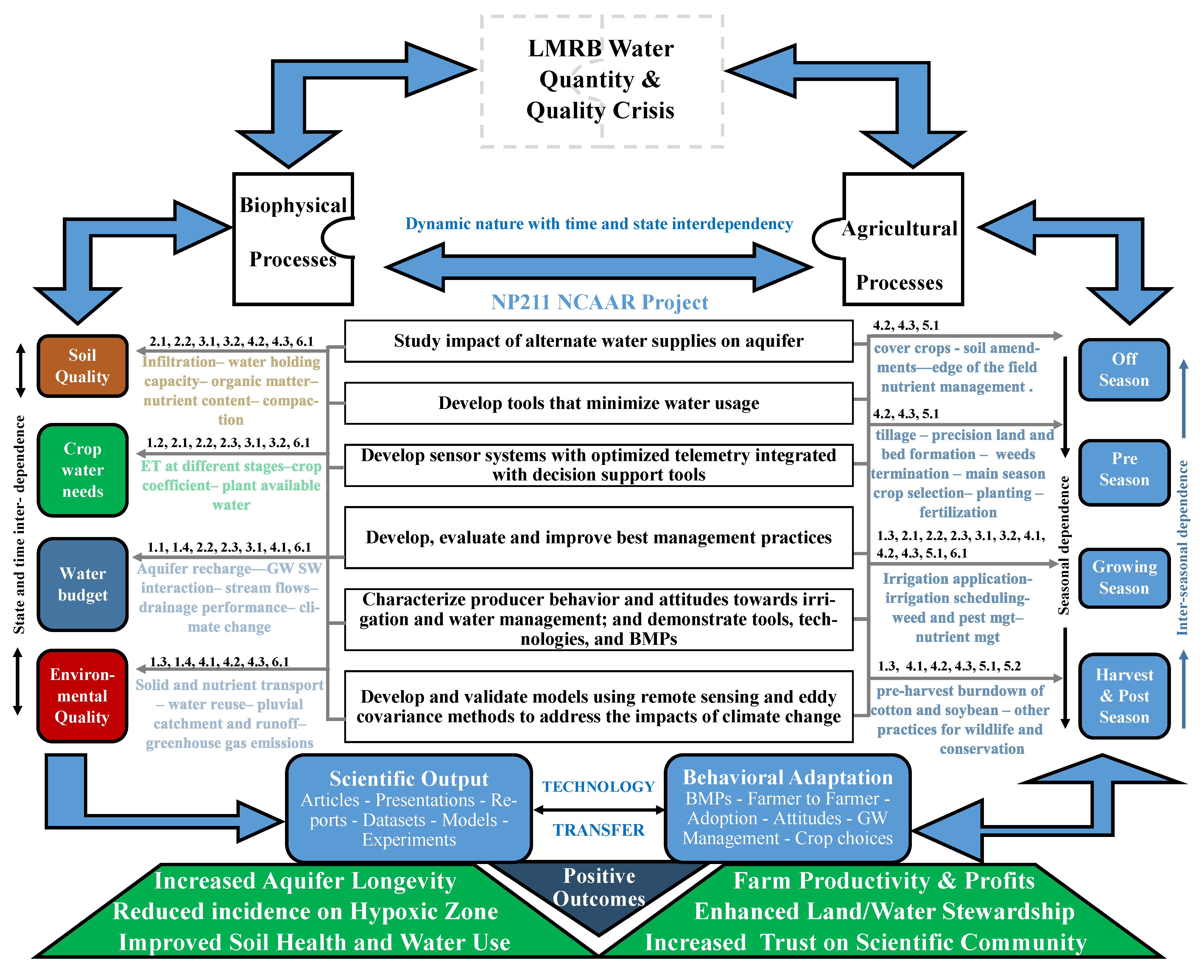
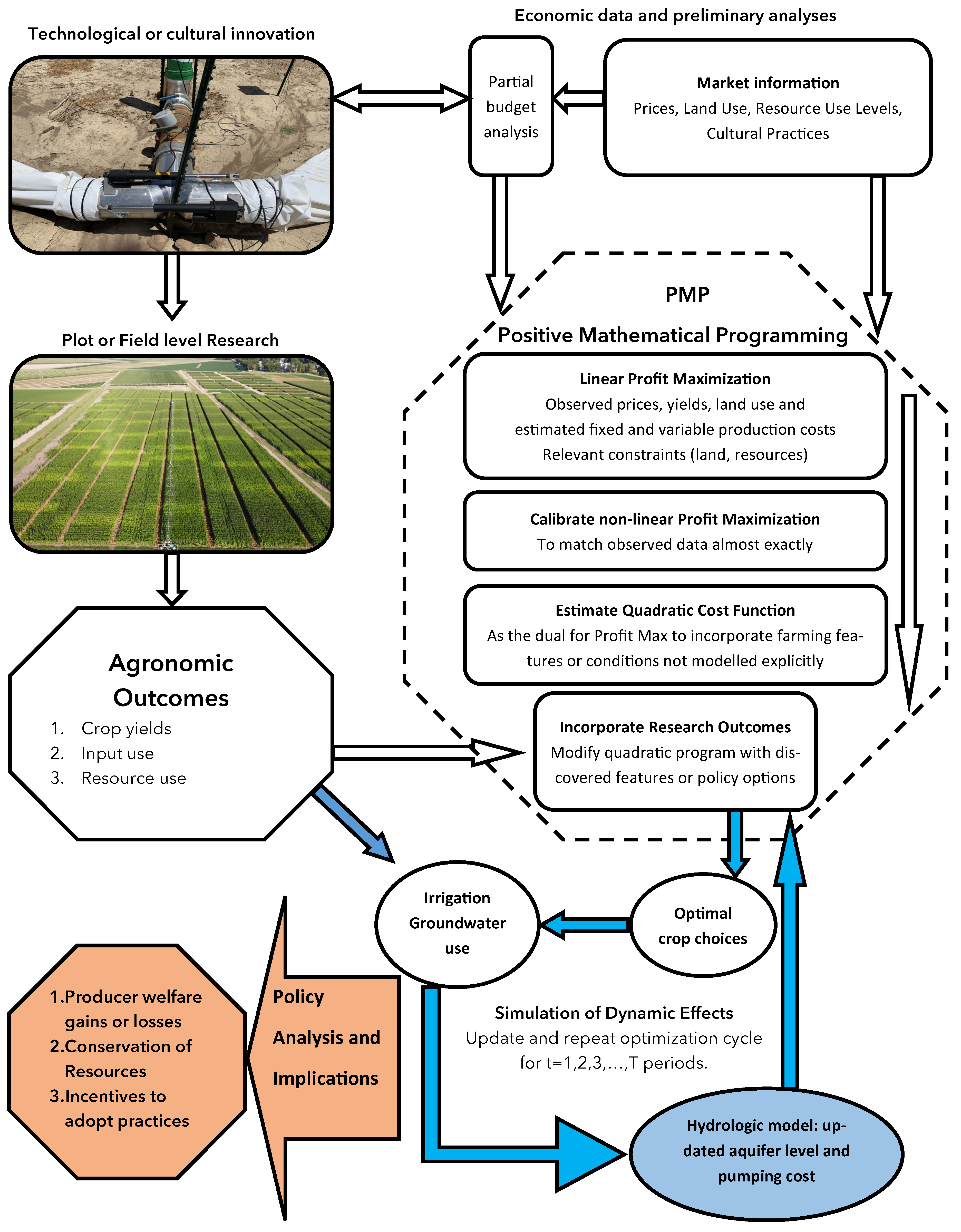
2. Integrating Multidisciplinary Research with Positive Mathematical Programming (PMP)

Disciplinary research offers important insights into processes within a specific domain and rarely incorporate interactions with other natural or social processes [24]. The way career researchers are evaluated by their academic departments tends to incentivize disjoint disciplinary research that results in shorter publication timelines and favors “preferred field-journals.” This effect is particularly evident with early career researchers (ECRs) who are underutilized in multidisciplinary research [25]. However, the scientific community is increasingly pushing and demanding research that integrates the insights of multiple disciplines to address global environmental challenges [24,26,27]. Far from being an integration of multidisciplinary models, positive mathematical programming is an economic analysis tool that allows the incorporation of otherwise disjoint disciplinary research into economic analyses and simulation of biophysical and socio-economic impacts that may result if certain practices or policies are adopted (see Figure 3).

Next, we describe the type of disciplinary research that can be fed into a PMP model to draw aquifer and policy implication insights.

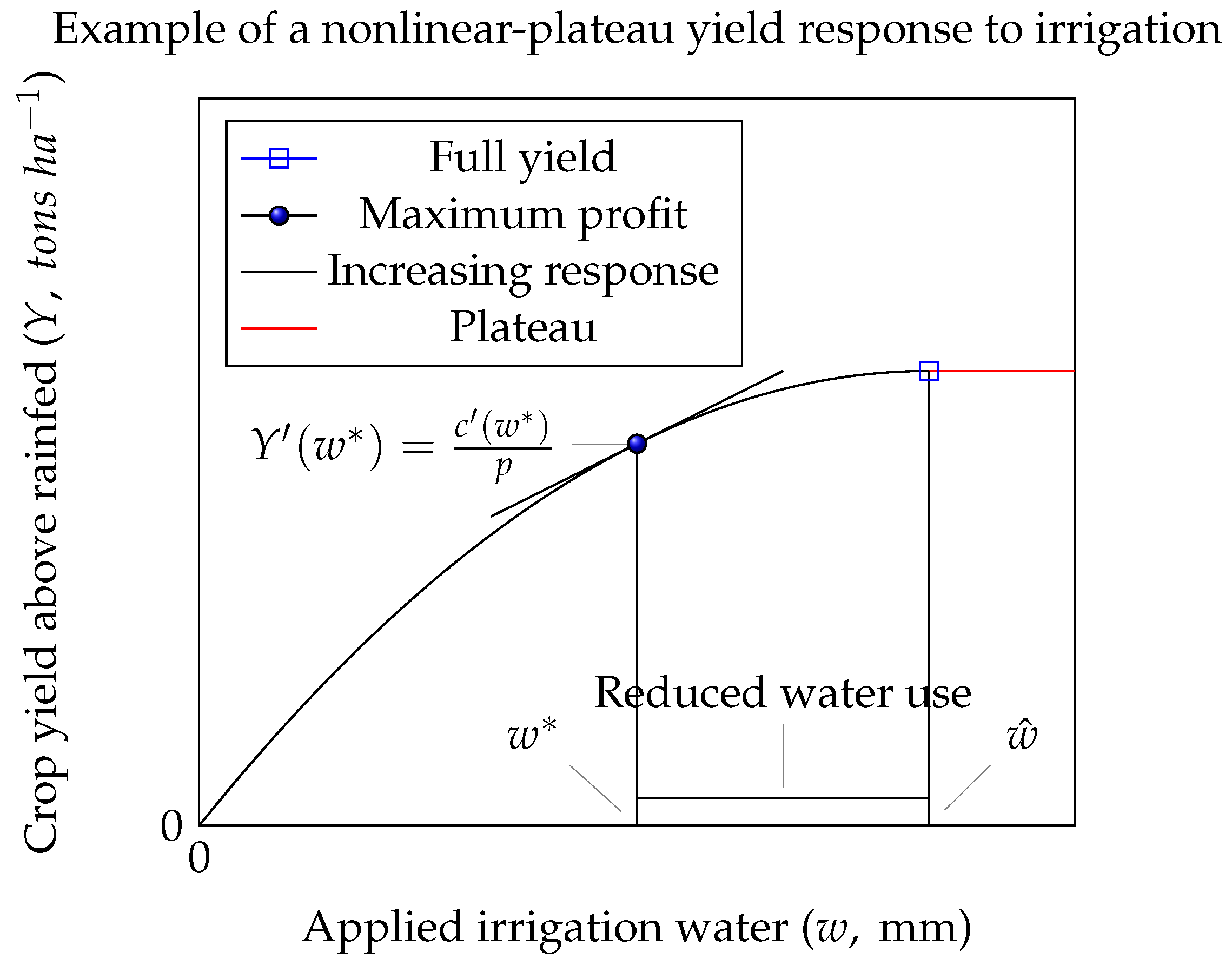
2.1. From Plot and Field-Level Research to Economic Behavior

Farmers operate in an increasingly risky environment and are likely to adopt practices that improve productivity (including water productivity), increase profits, or reduce risks [2]. Producers who want to be good stewards of their environment and are attracted to natural resource conservation still need assurances that the practices they are being told to adopt will not adversely affect their net incomes [28]. Plot and field-level research develops practices or prescriptions that hold the potential to deliver increased crop productivity, but often times it is hard to evaluate the impact the practice will have on marginal producer behavior. As the practices influence farmers’ behavior at the margin, wider implications would be expected at a regional or basin level.

Economists model producer behavior primarily as pursuing a business objective: maximizing profits or delivering a level of output at the minimum cost. Despite a multitude of other objectives, including cultural ones, the assumption of profit maximization is used because it predicts economic behavior reasonably well, particularly at some level of aggregation [29]. The decision regarding how input use, such as irrigation water, is determined “at the margin,” meaning the decision is made based on whether the treatment is expected to return a higher benefit than the cost of applying it. Figure 4 illustrates the concept with respect to water use: apply irrigation water until the benefit of the last unit applied equals its cost (marginal cost = marginal revenue). The response of crop yields to the amount of irrigation water applied depends on how much of other inputs have been used on the field (notably, fertilizer). However, because irrigation events occur after most of the other inputs have already been applied, it is acceptable to model crop yield response to water as a single-input function. The equations in Figure 4 reflect how plot and field-level results can be incorporated into an economic behavior model: if the innovation affects yields, production costs, or crop prices, then we can expect that it will affect farmers’ economic behavior.

With the insights of how agricultural innovations may affect producer behavior, the next step is to assess how the adoption of the innovation at the region or basin level will affect aquifer levels or environmental outcomes. Examples of agricultural research that could be incorporated in this framework abound. Plot level research on improved irrigation systems and technologies, and better agronomic management practices such as row spacing, cover crops, conservation tillage, and skip row irrigation are prime candidates.

The irrigation technologies that are available to the producers in the LMRB for increasing furrow irrigation application efficiency and irrigation water use efficiency include computer-hole-selection (PHAUCET: Pipe Hole and Universal Crown Elevation Tool or Pipe Planner); surge valves; soil moisture sensors, tailwater recovery systems, and recycling the runoff to reuse for irrigation; and sprinkler irrigation systems [8,10]. The soil moisture sensors, PHAUCET, and surge valves have been shown to improve in irrigation application efficiency of furrow irrigation systems. However, the application efficiency of the sprinkler systems is higher than that of furrow irrigation systems. However, there is little information available comparing water savings between a sprinkler irrigation system and a furrow irrigation system in which water conservation practices have been adopted to increase water use and application efficiencies (e.g., computer-hole-selection and moisture sensors). Adopting sprinkler irrigation systems could potentially increase water savings while increasing irrigation application efficiency and profits by reducing the costs of irrigation events.

Among conservation tillage practices, the use of strip tillage can reduce evaporation losses of water as it only disturbs 25 percent of the plow layer and allows retention of residues on the surface. Strip till shank can also break hardpans and reduce subsoil compaction. Retention of crop residues on the surface and reduction in subsoil compaction can allow better water infiltration in the soil, less runoff loss, and improve water availability for plant roots, which can increase water use efficiency by plants.

Skip row irrigation is another practice followed by some farmers on clay-textured soils in the MS Delta. Every other row is irrigated in the skip row irrigation strategy to save water and increase irrigation water use efficiency. Reducing the amount of water applied will result in lower fuel costs and higher net returns.

Cover crops can help with water conservation and improving soil health. Additionally, this practice can also increase water infiltration in soil, reduces evaporation losses, can increase the soil water holding capacity, reduces runoff and nutrient losses, and can increase nitrogen supply to the succeeding crop. Cover crops can reduce soil crusting and compaction, which are major constraints for crop production in the MS delta area. All these benefits of cover crops can reduce reliance on MRVAA for irrigation water needs. Improvements in irrigation water use efficiency with the use of cover crops have been reported by DeLaune et al. [30], Currie and Klocke [31].

2.2. Positive Mathematical Programming

Data on farms’ or farmers’ crop choices, practices, input or resource use, crop yields, and cost structures are generally unavailable in Mississippi, but exist at the county level. Consequently, the ability of the PMP methodology to model micro-economic behavior capable of reproducing the activity levels at the county level of aggregation is well suited to bridge the interdisciplinary and data availability barriers to basin-wide implications of agricultural experimental outcomes (see Figure 3).

The PMP-based dynamic simulation process is to:

• Use observed county-level data to formulate a constrained linear profit maximization model in which resource and input use and other resource, environmental or policy limitations are represented as constraints and the choice variable is crop acreage;
• Reformulate the problem as a nonlinear constrained optimization problem that calibrates almost exactly to the observed levels;
• Calibrate a quadratic function to capture desired production features (e.g.; water use) not included in the data or modelled explicitly;
• Implement a quadratic program including the estimated cost function as part of the objective function;
• Solve a dynamic model iteratively by updating aquifer levels based on periodic solutions to the quadratic program to produce the optimal land and water use choices.

The first step consists of using observed data to obtain the shadow prices on land use acres by solving the following problem for the observed period:

$$\begin{array}{cc}\hfill \underset{x_{rj}}{max}\pi & =\sum _r\sum _j\left(p_{rj}\times y_{rj}-c_{rj}\right)\times x_{rj};\end{array}$$

(1)

$$\begin{array}{cc}\hfill s.t.& \sum _j{x}_{rj}\le A_r=\sum _j{a}_{rj}\forall r;\end{array}$$

(2)

$$\begin{array}{cc}\hfill & a_{rj}-ϵ\le x_{rj}\le a_{rj}+ϵ\forall r,j;\end{array}$$

(3)

where $p_{rj}$ indicates the price of commodity j in region r at the time of the observed data; $y_{rj}$ indicates the observed yield level; $c_{rj}$ is the per-acre production costs; $x_{rj}$ is the choice variable for crop land allocation and $a_{rj}$ is the observed acreage for each crop; and $ϵ>\approx 0$ is a small perturbation in the observed acreage to produce calibrating shadow prices. Additional subscripts can be used to represent different production systems for which data are observed (e.g., different irrigation systems), or if only one region is analyzed, the r subscript can be used for that purpose. Crop prices are generally available from United States Department of Agriculture’s Economics, Statistics and Market Information System (USDA ESMIS) for specific elevators; acreage and average yield data are available from USDA NASS at the county level; and per acre cost of production by crop and production system is usually available via Crop Planning Budgets from the Extension Service at Land Grant Universities—in our case, the Department of Agricultural Economics at Mississippi State University, (https://www.agecon.msstate.edu/whatwedo/budgets.php, accessed on 8 August 2021).

The Lagrangean and first-order conditions for the problem for each region at the initial state are:

$$\begin{array}{c}\hfill {\mathcal{L}}_{0r}=\sum _j\left(p_j\times y{o}_j-c{o}_j\right)\times x_j+\lambda \left(A-\sum _j{x}_j\right)+\sum _j{\mu }_j\left(a_j+ϵ-x_j\right);\end{array}$$

(4)

$$\begin{array}{c}\hfill \frac{\partial {\mathcal{L}}_r}{\partial x_j}=p_j\times y{o}_j-c{o}_j-\lambda -{\mu }_j=0,\forall j;\end{array}$$

(5)

$$\begin{array}{c}\hfill \frac{\partial {\mathcal{L}}_r}{\partial \lambda }=A-\sum _j{x}_j=0;\end{array}$$

(6)

$$\begin{array}{c}\hfill {\mu }_j\left(a_j+ϵ-x_j\right)=0,\forall j;\end{array}$$

(7)

for which the solutions $x_j^{*}$ would be very close to the observed levels $a_j$ by construction.

For the second step, a cost function $C(w_{rj},x_{rj};{\alpha }_{rj},{\gamma }_{rj},{\delta }_{rj})$ to replace $c_{rj}$ in Equation (1) is estimated to incorporate additional desired features—i.e., water use, $w_j$. Additionally, we are interested in calibrating a crop yield function $Y_j(·)$ that captures the crop’s response to irrigation water application (or other inputs of interest) such that $Y_j\left(w_{rj}\right)=y_{rj}$ at the observed levels in the initial period.

A function that captures crop yield response to irrigation water applied can be specified as proposed by Martin et al. [32] and calibrated to reflect observed yields and water use [14,18]:

$$Y_j\left(w_{rj}\right)=Y{m}_{rj}+\left(Y{f}_{rj}-Y{m}_{rj}\right)\left[1-{\left(1-\frac{w_{rj}}{GI{R}_{rj}}\right)}^{-I{E}_{rj}}\right];$$

(8)

where $Ymrj$ is the minimum crop yield before irrigation water is applied; $Y{f}_{rj}$ is the fully-watered yield; $GI{R}_{rj}$ is the crop’s gross irrigation water requirement to achieve fully watered yield (given observed seasonal weather); and $I{E}_{rj}$ is the irrigation application efficiency. This function is estimated to reflect the initial observed levels of yield and water use.

The arguments for the function $Y_j\left(w_{rj}\right)$ is the first instance in which results from the plot or field-level research can be introduced. Practices that affect minimum yields (for example dryland), fully-watered yields, irrigation efficiency, or irrigation requirements can be incorporated in this formulation. In fact, the entire yield response function can be supplied by agronomic or plant physiology modeling as a component of the program.

Next, a cost function can be formulated as a linear function of the inputs and acreage [11,14,18]:

$$C(w_{rj},x_{rj};{\alpha }_{rj},{\gamma }_{rj},{\delta }_{rj})=(w_{rj}-w{o}_{rj}){\delta }_{rj}+{\alpha }_{rj}+0.5{\gamma }_{rj}{x}_{rj};$$

(9)

where $w{o}_{rj}$ is the initially observed rate of irrigation water application per acre. At the initial observation levels, the function collapses to

$$C(w{o}_{rj},x_{rj};{\alpha }_{rj},{\gamma }_{rj},{\delta }_{rj})={\alpha }_{rj}+0.5{\gamma }_{rj}{x}_{rj}=c{o}_{rj}.$$

(10)

The nonlinear program is now expressed as follows for the calibration problem:

$$\begin{array}{cc}\hfill \underset{x_{rj},w_{rj}}{max}{\pi }_r& =\sum _j\left(p_j\times Y_j\left(w_j\right)-C(w_j,x_j;{\alpha }_j,{\gamma }_j,{\delta }_j)\right)\times x_j;\end{array}$$

(11)

and first-order conditions:

$$\begin{array}{cc}\hfill \frac{\partial {\pi }_r}{\partial x_j}=& p_j\times Y_j\left(w_{rj}\right)-C(w_{rj},x_{rj};{\alpha }_{rj},{\gamma }_{rj},{\delta }_{rj})=0,\forall j;\end{array}$$

(12)

$$\begin{array}{cc}\hfill \frac{\partial {\pi }_r}{\partial w_j}=& p_j\times \frac{\partial Y_j\left(w_{rj}\right)}{\partial w_{rj}}-\frac{\partial C(w_{rj},x_{rj};{\alpha }_{rj},{\gamma }_{rj},{\delta }_{rj})}{\partial w_{rj}}=0,\forall j.\end{array}$$

(13)

The third step consists of combining the conditions from the two previous steps to match the initial observed levels of the variables of interest. From Equations (5) and (12) we obtain:

$${\alpha }_j+{\gamma }_j{a}_j=c{o}_j+{\mu }_j;$$

(14)

and Equation (10) is a second equality which can be used to solve for the two calibrating parameters (${\alpha }_j,{\gamma }_j$) since the values of the shadow prices ($\lambda ,{\mu }_j$) were obtained from the original program. The solutions are:

$$\begin{array}{cc}\hfill {\alpha }_j=& 2\frac{{\mu }_j}{x_j^{*}};and\end{array}$$

(15)

$$\begin{array}{cc}\hfill {\gamma }_j=& c{o}_j-{\mu }_i.\end{array}$$

(16)

The remaining calibrating parameter, ${\delta }_j$, can be found from Equation (9) and first-order condition (13) by taking the derivative of the yield response function $Y_j\left(w_j\right)$ specified in Equation (8):

$${\delta }_j=p_j\left(\frac{Y{f}_j-Y{m}_j}{I{E}_j\times GI{R}_j}\right){\left(1-\frac{w{o}_j}{GI{R}_j}\right)}^{(I{E}^{-1}-1)}.$$

(17)

The fourth step consists of preparing the cost function to adjust based on updated aquifer status. In this case, the pumping lift affects the pumping costs at time t [18]:

$${\mathsf{\Theta }}_t={\theta }_{et}\times 0.114\times \frac{TD{H}_t}{E{F}_t};$$

(18)

where ${\theta }_{et}$ is the price per unit of energy source e; $TD{H}_t$ is total dynamic head at time t; and $E{F}_t$ is energy efficiency of source e. $TDH$ is the sum of pumping lift $L_t$, which depends on aquifer levels at the end of period $t-1$; and pumping head, which converts the irrigation system pressurization requirement to feet of additional lift.

The resulting cost function takes the following form:

$$C(w_{jt},x_{jt})=(w_{jt}-w{o}_j)({\delta }_j+{\mathsf{\Theta }}_t)+{\alpha }_j+0.5{\gamma }_j{x}_{jt}.$$

(19)

A similar approach can be followed to study the effect of changing costs of other inputs or resources.

The final step consists of simulating the effects over time by the following aquifer equation of motion:

$$Lif{t}_t=Lif{t}_{t-1}+\frac{{\sum }_j{w}_{jt}\times x_{jt}-R}{A_s};$$

(20)

where R is the rate of net natural recharge of the aquifer and $A_s$ is the area in the region that overlays the aquifer multiplied by the aquifer specific yield. This aquifer formulation can be interpreted as a “localized” aquifer impact on the areas covered by the crops considered in the program. The change in lift distance over time is the amount of aquifer depletion (positive difference) or replenishment (negative change).

A word of caution with respect to PMP is that simulations should not be over very long time horizons because the calibration procedure seeks to fit results to the original conditions as much as possible. Over long periods of time, farmers can adapt in ways that make the original period observations become less relevant.

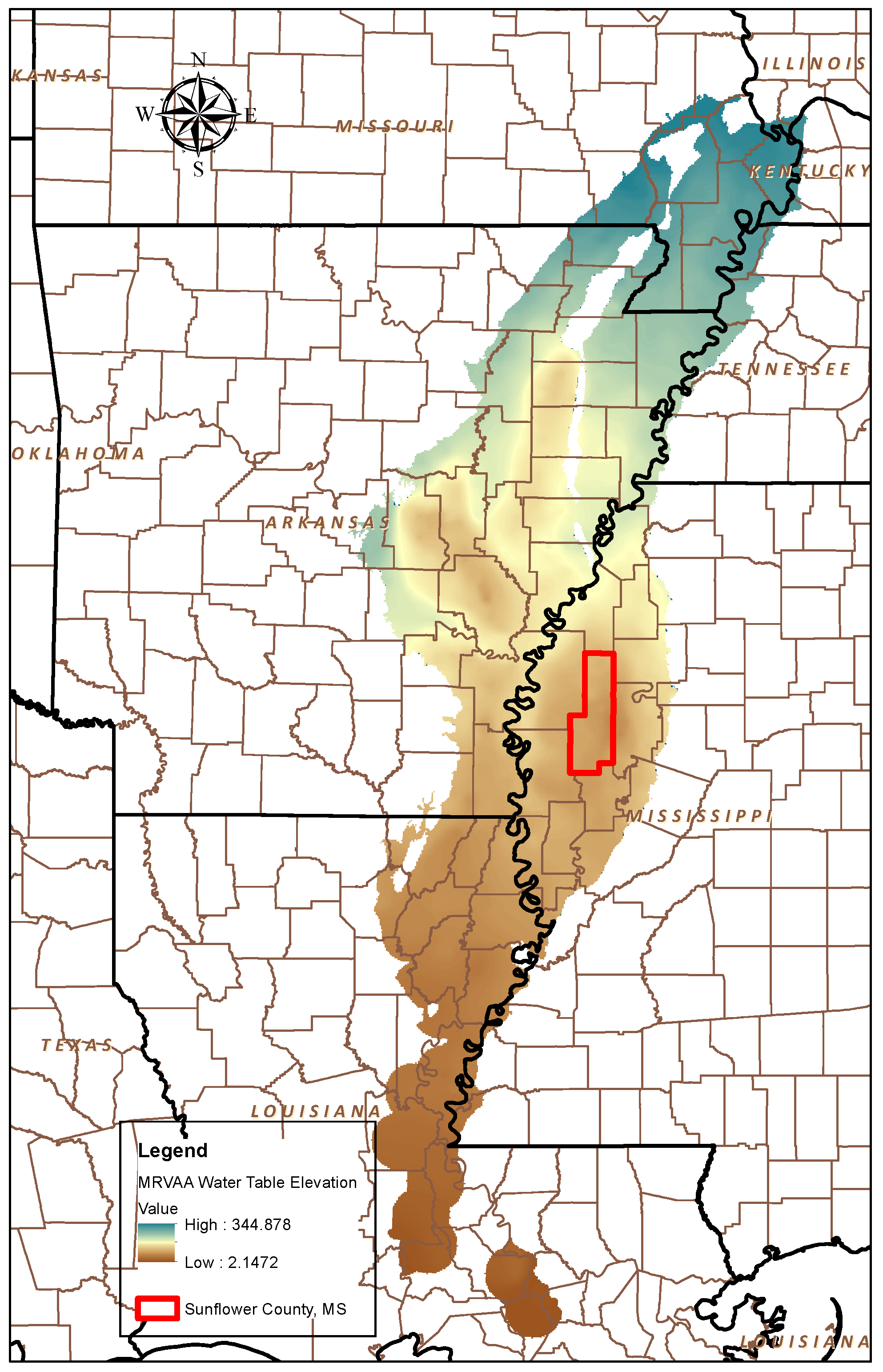
3. Illustrative Example: Improved Soybean Dryland Yields in Sunflower County, MS

To illustrate the methodology, we present a case study based on a hypothetical plot-level research that shows a 33 percent improvement in dryland soybean yields that do not involve changes in production costs relative to baseline conditions. Most agronomic studies do not include an economic analysis of this type of result, and few include only the partial budget analysis for the practice that tends to indicate how dryland soybean farmers would benefit from the practice. However, the PMP framework is able to expand the impact of the effect more systemically. For instance, an impact on irrigated soybeans is easily detectable via Equation (17). The yield improvement level was applied on the dynamic simulation state to both dryland soybean yields and to the minimum yield ($Y{m}_{soy}$) levels for soybeans.

3.1. Sunflower County, MS

To set up the model, we started with baseline information available from publicly accessible sources. County-level parameters are summarized in

Table 1. Model parameters for Sunflower County, MS.

Component	Parameter	Value
Aquifer	Surface elevation (FASL)	118
	Initial water table elev. (FASL)	77.91
	Aquifer base elevation (FASL)	−18.49
	Net recharge (R, acre-ft)	231,802
	Acres x specific yield ($A_S$)	89,344
Crop mix	Soybean share	77%
	Corn share	12%
	Rice share	4%
	Cotton share	7%
Irrigation	Application efficiency ($IE$)	0.54
Discount	Rate	0.03

and

Table 2. Summary of observed and estimated parameters for Sunflower County, MS.

Crop	Irrigation	Min.	Full-Water	Average	Water Use	Cost	Acres
		Yield	Yield	Yield	(ft/acre)	($\mathit{\$}/$acre)
Corn	Furrow	114 bu/a	280 bu/a	220 bu/a	0.83	680	27,857
	Dryland			170 bu/a		585	8343
Soybean	Furrow	26 bu/a	82 bu/a	77 bu/a	1.16	498	158,144
	Dryland			57 bu/a		404	76,356
Cotton	Furrow	1090 lb/a	1800 lb/a	1479 lb/a	0.5	924	16,958
	Dryland			1261 lb/a		833	3747
Rice	Flood	99 bu/a	253 bu/a	228 bu/a	2.7	817	13,830

. It fully overlies an acute depression of the MRVAA water table –which has drawn concern from producers and federal and state agencies [33]. Due to concerns about MRVAA depletion, Mississippi Governor Phil Bryant established the Governor’s Delta Sustainable Water Resources Task Force in November of 2011 to ensure the future sustainability of water resources in the Delta [34].

Sunflower County, MS, is in the center of the Delta area of Mississippi (red contour in Figure 2). The row-crop agriculture in the county is widely representative of the Delta. Consequently, the area is ideal for a representative agent type of model such as this, as it is big enough to draw conclusions about the aquifer but small enough that a simplified aquifer model is capable of capturing its most important dynamics [35].

Table 2 summarizes the selected variables in the model for Sunflower County, MS. USDA NASS data for 2017 is the latest available so we match the rest of the data to observations for that year. Price and cost information was obtained from the Mississippi State University, 2017 Delta Crop Planning Budgets, https://www.agecon.msstate.edu/whatwedo/budgets.php, accessed on 8 August 2021. Crop acreage and average yields were obtained from USDS NASS [36]. Information on minimum and maximum yields was obtained from expert opinion and from Mississippi State University various variety trials in 2017. Average irrigation water use by crop was calculated from Mississippi Department of Environmental Quality’s (MDEQ) voluntary well metering program and verified with information from experimental on-farm NCAAR data. Average irrigation efficiency was based on Bryant et al. [8], and Spencer et al. [10]. Parameters to calculate gross irrigation requirements ($GIR$) were obtained from Tang et al. [37].

The calibrated problem was modified, and the results simulated over 20 years and compared to the baseline results. The results of the calibrated problem which was only updated for aquifer depletion are called the “calibrated” scenario, and the program modified to reflect both the updated state of the aquifer and the increase in dryland soybean yields is called the “shock” scenario.

3.2. Results and Discussion for an Illustrative Example

The dynamic simulation was run under the two scenarios for 20 simulated years. The “calibrated” scenario was the modified program that included the ability to update the status of the aquifer, which affected pumping lifts over time, which in turn affected costs. The “shock” scenario was also modified to update pumping lift, but also incorporated an improvement in the level of dryland soybean yields (affecting minimum yield as well).

Table 3. Salient Positive mathematical programming results for 20 simulated years, by crop and practice.

Crop	Irrigation	Acres		Water Use (acre-ft)		Profits ($\mathit{\$}/$year)
		Year 1	Year 20	Year 1	Year 20	Year 1	Year 20
Corn/calib.	Furrow	27,873	27,620	23,135	22,789	22.8M	22.5M
	Dryland	8343	8343	0	0	5.3M	5.3M
Corn/shock	Furrow	23,752	23,775	19,715	19,757	19.4M	19.4M
	Dryland	4995	4971	0	0	3.19M	3.18M
Soybean/calib.	Furrow	158,142	157,490	184,077	182,783	117.2M	116.6M
	Dryland	76,356	76,356	0	0	43.8M	43.8M
Soybean/shock	Furrow	144,668	144,707	168,393	168,536	107.2M	107.3M
	Dryland	109,167	109,094	0	0	83.2M	83.2M
Cotton/calib.	Furrow	16,913	16,592	8457	8235	16.4M	16.1M
	Dryland	3747	5110	0	0	3.1M	4.3M
Cotton/shock	Furrow	9811	9827	4905	4920	9.5M	9.5M
	Dryland	≈0	≈0	0	0	0	0
Rice/calib.	Flood	13,859	13,723	37,420	36,799	14.9M	14.8M
Rice/shock	Flood	12,841	12,861	34,670	34,772	13.9M	13.9M

summarizes select results by crop.

As expected, dryland soybean acreage and profitability increased with the shock. This result shows the limits of typical economic analysis of agronomic research. However, PMP allows one to identify additional implications with respect to the calibrated baseline. The increase in soybean dryland acreage comes at the expense not only of the irrigated soybean acreage, but also from all other crops including virtually eliminating dryland cotton cultivation.

An actual analysis of the idiosyncrasies of cotton production would caution against this implication due to the level of specialization involved in cotton production which would make it hard for a cotton farmer to immediately convert to another row crop. Notice that in the calibrated scenario, the program allocated more acreage to dryland cotton (see year 1 vs. year 20 land allocation).

With the significant increase in the profitability of dryland soybean, the corresponding increased land allocation to its cultivation result in a net replenishment of the localized aquifer (see

Table 4. Farmer welfare, aggregate water use, and localized changes in groundwater levels (over 20 years).

Scenario	Net Present Value	Aggregate	Change in
	of Farm Profits	Water Use (acre-ft)	Aquifer Level (ft)
Calibrated scenario	$\$3.42$ billion	5 million	4.5 ft decrease
Yield shock scenario	$\$3.62$ billion	4.6 million	0.9 ft increase

). This aquifer replenishment allowed a sustainable increase in all the irrigated acreage over time, although never reaching those under the calibrated scenario.

The other important extension of the analysis was with respect to the aggregate results, which allowed us to draw insights at regional and basin-wide scales. Table 4 summarizes the aggregate producer welfare results expressed as the net present value (NPV) of the sum of the stream of profits under the two scenarios. The NPV was calculated using a discount factor that incorporated the current FSA Loan rate for Farm Ownership loans of three percent.

The yield shock introduced produced almost $\$200$ million more in producer welfare while reducing aggregate water use by over 400 k acre-ft. The health of the aquifer was substantially better under the shock scenario, which resulted in a slightly replenished aquifer. The implications for sustainability are important, as they indicate a substantial amount of sustainable available water to expand irrigated agriculture (remember that the program constrains the total acreage to the initially observed). The aquifer level presents a difference of over 6.4 ft between the two scenarios after 20 years. Given the improvement in both producer welfare and aquifer levels, research to improve dryland yields and provide incentives for conversion to dryland varieties appears an attractive target for public policy and funds.

4. Conclusions

Positive mathematical programming offers the ability to integrate compartmentalized disciplinary research to produce deeper insights on the effects and repercussions experimental plot or field-level research can have on regional or basing wide producer welfare and natural resource conditions. The typical economic analysis of agronomic research is limited to the partial budget analysis associated with implementing an experimental practice. PMP includes and extends the analysis by showing implications on the wider agricultural system including input and resource use allocations across crops and practices.

We presented a clear step-by-step guide to implement the methodology employing straight-forward mathematical optimization techniques and including ways in which the programs can be modified to incorporate unobserved features of interest. The application of this methodology would make highly disciplinary research more relevant across disciplines and to various stakeholders who could more easily assess the implications of the agricultural experimental practices proposed and the eventual technology transfer as producers adopt them.

A caveat of PMP is that the resulting programs, by design, try to produce allocations that mimic as much as possible those observed in the initial period on which the program is calibrated. However, as evidenced by the hypothetical case presented, the directions of change are readily identified.

The procedure described in Section 2.2 can be implemented in any quantitative or statistical analysis software. The results for the example presented were produced using MatLab’s linprog and quadprog optimization tools.

References

1. Yasarer, L.M.; Taylor, J.M.; Rigby, J.R.; Locke, M.A. Trends in land use, irrigation, and streamflow alteration in the Mississippi River Alluvial Plain. Front. Environ. Sci. 2020, 8, 66. [Google Scholar] [CrossRef]
2. Quintana-Ashwell, N.E.; Gholson, D.M.; Krutz, L.J.; Henry, C.G.; Cooke, T. Adoption of Water-Conserving Irrigation Practices among Row-Crop Growers in Mississippi, USA. Agronomy 2020, 10, 1083. [Google Scholar] [CrossRef]
3. Quintana-Ashwell, N.E.; Anapalli, S.S.; Pinnamaneni, S.R.; Kaur, G.; Reddy, K.N.; Fisher, D.K. Profitability of twin-row planting and skip-row irrigation in a humid climate. Agron. J. 2021, in press. [Google Scholar] [CrossRef]
4. Elliott, J.; Deryng, D.; Müller, C.; Frieler, K.; Konzmann, M.; Gerten, D.; Glotter, M.; Flörke, M.; Wada, Y.; Best, N.; et al. Constraints and potentials of future irrigation water availability on agricultural production under climate change. Proc. Natl. Acad. Sci. USA 2014, 111, 3239–3244. [Google Scholar] [CrossRef] [Green Version]
5. Pinnamaneni, S.R.; Anapalli, S.S.; Reddy, K.N.; Fisher, D.K.; Quintana Ashwell, N.E. Assessing irrigation water use efficiency and economy of twin-row soybean in the Mississippi Delta. Agron. J. 2020, 112, 4219–4231. [Google Scholar] [CrossRef]
6. Pinnamaneni, S.R.; Anapalli, S.S.; Reddy, K.N.; Fisher, D.K. Effects of irrigation and planting geometry on cotton productivity and water use efficiency. J. Cotton Sci. 2020, 24, 2–96. [Google Scholar]
7. Henry, W.B.; Krutz, L.J. Water in agriculture: Improving corn production practices to minimize climate risk and optimize profitability. Curr. Clim. Chang. Rep. 2016, 2, 49–54. [Google Scholar] [CrossRef] [Green Version]
8. Bryant, C.; Krutz, L.; Falconer, L.; Irby, J.; Henry, C.; Pringle, H.; Henry, M.; Roach, D.; Pickelmann, D.; Atwill, R.; et al. Irrigation water management practices that reduce water requirements for Mid-South furrow-irrigated soybean. Crop. Forage Turfgrass Manag. 2017, 3, 1–7. [Google Scholar] [CrossRef] [Green Version]
9. Wood, C.; Krutz, L.; Falconer, L.; Pringle, H.; Henry, B.; Irby, T.; Orlowski, J.; Bryant, C.; Boykin, D.; Atwill, R.; et al. Surge irrigation reduces irrigation requirements for soybean on smectitic clay-textured soils. Crop. Forage Turfgrass Manag. 2017, 3, 1–6. [Google Scholar] [CrossRef]
10. Spencer, G.; Krutz, L.; Falconer, L.; Henry, W.; Henry, C.; Larson, E.; Pringle, H.; Bryant, C.; Atwill, R. Irrigation Water Management Technologies for Furrow-Irrigated Corn that Decrease Water Use and Improve Yield and On-Farm Profitability. Crop. Forage Turfgrass Manag. 2019, 5, 1–8. [Google Scholar] [CrossRef] [Green Version]
11. Howitt, R.E. Positive Mathematical Programming. Am. J. Agric. Econ. 1995, 77, 329–342. [Google Scholar] [CrossRef]
12. Heckelei, T.; Britz, W. Models based on positive mathematical programming: State of the art and further extensions. In Proceedings of the European Association of Agricultural Economists (EAAE), Parma, Italy, 2–5 February 2005. [Google Scholar]
13. Qureshi, M.E.; Whitten, S.M.; Kirby, M. A multi-period positive mathematical programming approach for assessing economic impact of drought in the Murray–Darling Basin, Australia. Econ. Model. 2014, 39, 293–304. [Google Scholar] [CrossRef]
14. Garay-Armoa, P.V. The Impact of Climate Change on the Effectiveness of Water Conservation Policies in Western Kansas and the Ogallala Aquifer. Ph.D. Thesis, Kansas State University, Manhattan, KS, USA, 2015. [Google Scholar]
15. Koundouri, P. Current issues in the economics of groundwater resource management. J. Econ. Surv. 2004, 18, 703–740. [Google Scholar] [CrossRef] [Green Version]
16. Koundouri, P. Potential for groundwater management: Gisser-Sanchez effect reconsidered. Water Resour. Res. 2004, 40. [Google Scholar] [CrossRef] [Green Version]
17. Pulido-Velazquez, M.; Andreu, J.; Sahuquillo, A.; Pulido-Velazquez, D. Hydro-economic river basin modelling: The application of a holistic surface–groundwater model to assess opportunity costs of water use in Spain. Ecol. Econ. 2008, 66, 51–65. [Google Scholar] [CrossRef]
18. Clark, M.K. Effects of High Commodity Prices on Western Kansas Crop Patterns and the Ogallala Aquifer. Ph.D. Thesis, Kansas State University, Manhattan, KS, USA, 2009. [Google Scholar]
19. Esteban, E.; Albiac, J. The problem of sustainable groundwater management: The case of La Mancha aquifers, Spain. Hydrogeol. J. 2012, 20, 851–863. [Google Scholar] [CrossRef]
20. Lambert, L.H.; English, B.C.; Clark, C.C.; Lambert, D.M.; Menard, R.J.; Hellwinckel, C.M.; Smith, S.A.; Papanicolaou, A. Local effects of climate change on row crop production and irrigation adoption. Clim. Risk Manag. 2021, 32, 100293. [Google Scholar] [CrossRef]
21. Aistrup, J.A.; Bulatewicz, T.; Kulcsar, L.J.; Peterson, J.M.; Welch, S.M.; Steward, D.R. Conserving the Ogallala Aquifer in southwestern Kansas: From the wells to people, a holistic coupled natural–human model. Hydrol. Earth Syst. Sci. 2017, 21, 6167–6183. [Google Scholar] [CrossRef] [Green Version]
22. MacEwan, D.; Cayar, M.; Taghavi, A.; Mitchell, D.; Hatchett, S.; Howitt, R. Hydroeconomic modeling of sustainable groundwater management. Water Resour. Res. 2017, 53, 2384–2403. [Google Scholar] [CrossRef]
23. Dale, L.L.; Dogrul, E.C.; Brush, C.F.; Kadir, T.N.; Chung, F.I.; Miller, N.L.; Vicuna, S.D. Simulating the impact of drought on California’s Central Valley hydrology, groundwater and cropping. Br. J. Environ. Clim. Chang. 2013, 3, 271. [Google Scholar] [CrossRef]
24. Bulatewicz, T.; Allen, A.; Peterson, J.M.; Staggenborg, S.; Welch, S.M.; Steward, D.R. The simple script wrapper for OpenMI: Enabling interdisciplinary modeling studies. Environ. Model. Softw. 2013, 39, 283–294. [Google Scholar] [CrossRef] [Green Version]
25. Sobey, A.; Townsend, N.; Metcalf, C.; Bruce, K.; Fazi, F.M. Incorporation of Early Career Researchers within multidisciplinary research at academic institutions. Res. Eval. 2013, 22, 169–178. [Google Scholar] [CrossRef] [Green Version]
26. Parson, E.A. Integrated assessment and environmental policy making: In pursuit of usefulness. Energy Policy 1995, 23, 463–475. [Google Scholar] [CrossRef]
27. Rotmans, J.; Van Asselt, M. Integrated assessment: A growing child on its way to maturity. Clim. Chang. 1996, 34, 327–336. [Google Scholar] [CrossRef]
28. Adams, K.; Kovacs, K. The adoption rate of efficient irrigation practices and the consequences for aquifer depletion and further adoption. J. Hydrol. 2019, 571, 244–253. [Google Scholar] [CrossRef]
29. Pindyck, R.; Rubinfeld, D. Microeconomics, 7th ed.; Prentice Hall: Upper Saddle River, NJ, USA, 2009. [Google Scholar]
30. DeLaune, P.; Mubvumba, P.; Ale, S.; Kimura, E. Impact of no-till, cover crop, and irrigation on Cotton yield. Agric. Water Manag. 2020, 232, 106038. [Google Scholar] [CrossRef]
31. Currie, R.S.; Klocke, N.L. Impact of a terminated wheat cover crop in irrigated corn on atrazine rates and water use efficiency. Weed Sci. 2005, 53, 709–716. [Google Scholar] [CrossRef]
32. Martin, D.L.; Watts, D.G.; Gilley, J.R. Model and production function for irrigation management. J. Irrig. Drain. Eng. 1984, 110, 149–164. [Google Scholar] [CrossRef] [Green Version]
33. Barlow, J.R.; Clark, B.R. Simulation of Water-Use Conservation Scenarios for the Mississippi Delta Using an Existing Regional Groundwater Flow Model; US Department of the Interior, US Geological Survey: Reston, VA, USA, 2011.
34. Bryant, P. Mississippi Governor Executive Order 1341. 2014. Available online: https://www.sos.ms.gov/communications-publications/executive-orders (accessed on 22 October 2021).
35. Brozović, N.; Sunding, D.L.; Zilberman, D. On the spatial nature of the groundwater pumping externality. Resour. Energy Econ. 2010, 32, 154–164. [Google Scholar] [CrossRef] [Green Version]
36. USDA-NASS. Mississippi Soybean County Estimates; National Agricultural Statistics Service, United States Department of Agriculture: Washington, DC, USA, 2020.
37. Tang, Q.; Feng, G.; Fisher, D.; Zhang, H.; Ouyang, Y.; Adeli, A.; Jenkins, J. Rain water deficit and irrigation demand of major row crops in the Mississippi Delta. Trans. ASABE 2018, 61, 927–935. [Google Scholar] [CrossRef]
Figure 1. Conceptual diagram of USDA ARS NP211 that funds the National Center for Alluvial Aquifer Research (NCAAR).
Agronomy 11 02204 g001
Figure 2. Potentiometric map of the Mississippi River Valley Alluvial Aquifer based on U.S. Geological Survey data from 2016.
Agronomy 11 02204 g002
Figure 3. A diagram depicting multidisciplinary research using positive mathematical programming (PMP) to integrate plot-level research into basin-wide models and drawing policy implications.
Agronomy 11 02204 g003
Figure 4. Illustration of the relationship among crop yield, applied irrigation water, and profits.
Agronomy 11 02204 g004