Article

Evaluation of a Stereo Vision System for Cotton Row Detection and Boll Location Estimation in Direct Sunlight

1
College of Engineering, University of Georgia, Athens, GA 30602, USA
2
Department of Entomology, University of Georgia, Tifton, GA 31793, USA
3
Department of Crop and Soil Sciences, University of Georgia, Tifton, GA 31793, USA
4
Cotton Incorporated, Cary, NC 27513, USA
*
Authors to whom correspondence should be addressed.
Agronomy 2020, 10(8), 1137; https://doi.org/10.3390/agronomy10081137
Submission received: 1 July 2020 / Revised: 31 July 2020 / Accepted: 3 August 2020 / Published: 5 August 2020

Abstract

:
Cotton harvesting is performed by using expensive combine harvesters which makes it difficult for small to medium-size cotton farmers to grow cotton economically. Advances in robotics have provided an opportunity to harvest cotton using small and robust autonomous rovers that can be deployed in the field as a “swarm” of harvesters, with each harvester responsible for a small hectarage. However, rovers need high-performance navigation to obtain the necessary precision for harvesting. Current precision harvesting systems depend heavily on Real-Time Kinematic Global Navigation Satellite System (RTK-GNSS) to navigate rows of crops. However, GNSS cannot be the only method used to navigate the farm because for robots to work as a coordinated multiagent unit on the same farm because they also require visual systems to navigate, avoid collisions, and to accommodate plant growth and canopy changes. Hence, the optical system remains to be a complementary method for increasing the efficiency of the GNSS. In this study, visual detection of cotton rows and bolls was developed, demonstrated, and evaluated. A pixel-based algorithm was used to calculate and determine the upper and lower part of the canopy of the cotton rows by assuming the normal distribution of the high and low depth pixels. The left and right rows were detected by using perspective transformation and pixel-based sliding window algorithms. Then, the system determined the Bayesian score of the detection and calculated the center of the rows for the smooth navigation of the rover. This visual system achieved an accuracy of 92.3% and an F1 score of 0.951 for the detection of cotton rows. Furthermore, the same stereo vision system was used to detect the location of the cotton bolls. A comparison of the cotton bolls’ distances above the ground to the manual measurements showed that the system achieved an average R2 value of 99% with a root mean square error (RMSE) of 9 mm when stationary and 95% with an RMSE of 34 mm when moving at approximately 0.64 km/h. The rover might have needed to stop several times to improve its detection accuracy or move more slowly. Therefore, the accuracy obtained in row detection and boll location estimation is favorable for use in a cotton harvesting robotic system. Future research should involve testing of the models in a large farm with undefoliated plants.

1. Introduction

Cotton harvesting is heavily dependent on large machinery with human operators. These massive machines are costly to maintain and expensive to own. The emergence of modern technologies in robotics provides an opportunity to explore alternative harvesting methods [1,2,3,4,5]. The introduction of small, intelligent, multiagent machines in farming will be an asset to farmers. Swarms can be scalable to the size of the farm, and each machine can be low-cost, multipurpose, and reprogrammable for the task at hand. Smaller machines can also reduce the risk of severe injuries and fatalities, sometimes experienced with large field equipment [1,6]. With modular attachments and selectable programming, these small intelligent machines can be used for multiple tasks, such as precision weeding, chemical application, planting, harvesting, and scouting [7].
Recently, several harvesting robots have been developed and reported to be research tools or for production agriculture, such as harvesting robots for cucumbers [8], grapes [9,10], apples [11], tomatoes [12], strawberries [13], kiwifruit [14], and sweet peppers [15,16]. Most of these robots are slow to pick fruit because of the technology and technique used to identify, locate, and pick the product. The faster robotic machines use a prescription map and multiple robotic arms to harvest many fruits at once [14,17], which is, in part, due to the difficulty that arises from trying to control the complex farming environment that has variable lighting, dusty conditions, and machine vibrations, all of which produce “noise” to the imaging system [14,15,16]. These impending conditions pose challenges even to current machine vision technologies.
Plant rows are discernible when cotton plants are seedlings, and the canopy overlaps around 8–10 weeks after planting. Ref. [2] conducted a study to detect rows in young crops using a stereo system and provided an excellent baseline for visual detection of the canopy, an advancement in machine vision research for row crop detection as compared with color-based detection algorithms proposed in other studies [18,19,20]. Ref. [5] proposed the use of LiDAR sensors and red-green-blue (RGB) cameras to detect small row crops.
The cotton harvesting rover is expected to be deployed in nondefoliated plants as soon as the cotton bolls begin to open. Careful navigation in a fully-grown canopy is required so that the bolls are not knocked to the ground and also are easily located and tracked for picking by the robotic harvester arm. Most cotton in the USA is planted with row spacing ranging from 30 to 40 inches (76 to 101.6 cm) [21]. Therefore, the harvesting machine must make sure that the tires are close to the center of the row spacing. For human-driven tractors, Real-Time Kinematic Global Navigation Satellite System (RTK-GNSS) is very accurate and can be used to continue following the same course with centimeter accuracy [2,22]. However, for self-navigation, visual perception is also needed to avoid field obstructions. As such, it is important to use visual perception to give the rover an alternative to RTK-GNSS in case it fails and to provide a complementary view of the environment.
RTK-GNSS navigation is challenged by the signal loss during operation resulting from attenuation around buildings, tree cover, and other obstructions [22]. This requires farmers to use an expensive RTK-GNSS system. Additionally, deployment of a swarm of robots that coordinate their work requires preprogramming to ensure that obstacles and machines avoid collisions. Therefore, the use of a camera and simple RTK-GNSS must be sufficient to achieve safe, real-time navigation for farm vehicles traveling over the plants by detecting the canopy and a clear path. There are other sensors such as the LiDAR that can be used in this operation. However, as we expect, the machine to work in daylight and over plants, i.e., RGB cameras is sufficient. LiDAR which is an expensive tool as compared with RGB cameras has shown success when small robots navigate at night between large plants [22]. However, ref. [23] evaluated the performance of the algorithm using a RGB camera with artificial lighting conditions and found that their algorithm performed very well for the detection of apples when artificial lighting conditions were used.
Some machine vision techniques using LiDAR have been developed to determine the height of cotton plants, but not “on the go,” which is a real-time harvesting requirement [24]. Machine vision systems for cotton harvesting are not yet available, but some preliminary research has been conducted by [1,25,26]. Ref. [25] were able to develop an imaging system for cotton recognition using color segmentation methods and detected cotton bolls at an accuracy of 85%. Furthermore, some work for the visual navigation of a cotton harvesting rover has been done using the Otsu method and noise filtering vision techniques [27]. Research in India attempted to design an automatic cotton harvesting rover that used image processing techniques to acquire features and perform modeling and matching, but a commercial product was not developed [28]. To date, no research has been reported to determine the absolute location of the cotton bolls or cotton rows for robotic purposes.
The location of cotton bolls is the vertical and horizontal distances of a boll from the center of the camera’s carrying platform. This location is vital for controlling the position of a harvesting manipulator designed to pick individual cotton bolls. However, to achieve this harvesting action, the machines require high performing computing and imaging resources. Present computing technologies can provide a quick solution for cotton boll localization and mapping used to position the robot’s end effector for harvesting. An x-y Cartesian robotic arm can move in two axes, i.e., up/down and left/right [29,30]. However, an imaging system is required to predetermine the postions of the cotton bolls and send that information to the machine, then, the robot manipulator can plan and move to pick the cotton bolls [29,30]. Our motivation is to contribute to efforts in the development of the cotton harvesting robot by developing algorithms that localize the rover according to the planting style of the cotton plant.
The main objective of this study was to develop and evaluate a model to detect the rows and cotton bolls in a cotton field and test the performance of the model. A model using a stereo camera is proposed to guide a cotton harvesting robot in rows and detect cotton bolls. The same camera was used to locate bolls and detect cotton rows. The specific objectives of this study were the following;
  • Develop and evaluate a model to measure the location of the cotton bolls using the stereo camera in direct sunlight;
  • Develop and evaluate a model to detect cotton rows using a stereo camera in direct sunlight.

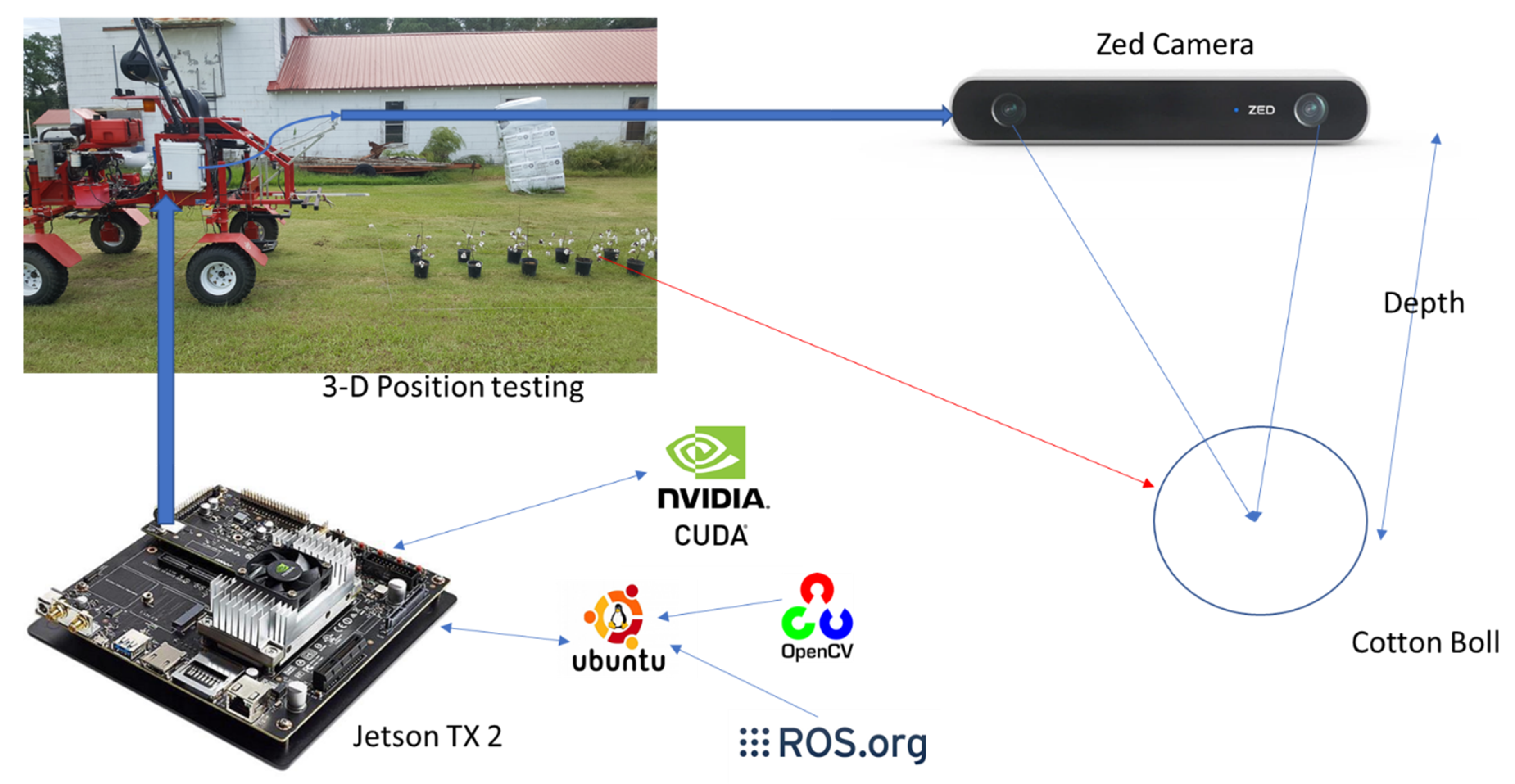
2. Materials and Methods
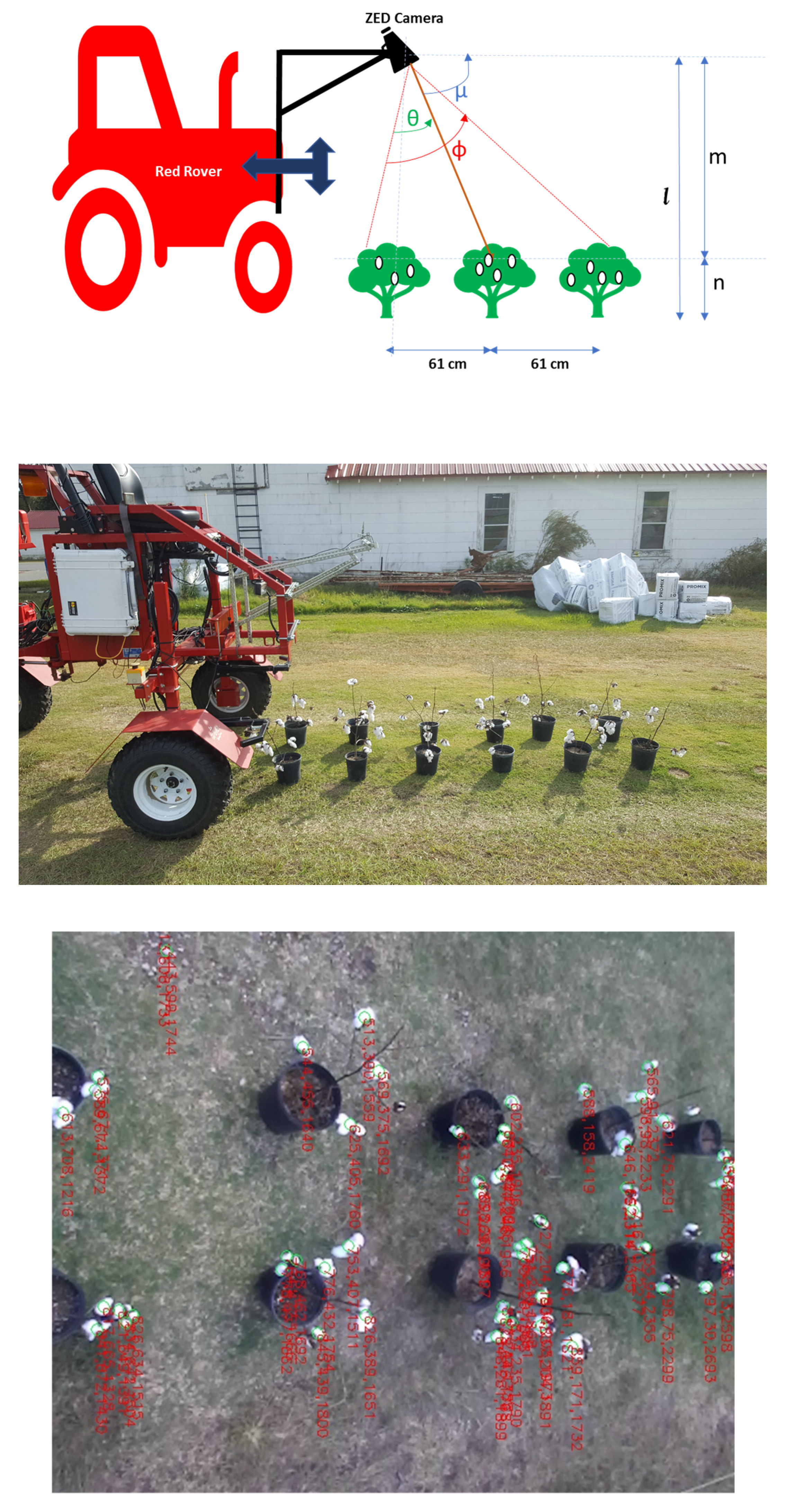
2.1. Materials

The red custom-built articulated rover (West Texas Lee Corp., Lubbock, Texas) with modifications to meet the field conditions, navigation, and obstacle avoidance requirements of an unstructured (such as open field and end of the row) and a structured field was used to detect cotton bolls and rows [1,6]. The rover was 340 cm long and front and back parts were 145 and 195 cm long, respectively. The rover’s height and width could be adjusted to a maximum of 122 and 234 cm, respectively. The rover tires were 91 cm from the center of the vehicle. The rover was 212 cm wide, with a tire width of 30 cm. The four tires had a radius of 30.48 cm and a circumference of 191.51 cm. The rover had a ground clearance of 91 cm. The rover was mounted with a stereo camera (ZED, Stereo labs Inc, San Francisco, CA, USA) and a rugged development kit, NVIDIA Jetson TX2 (NVIDIA Jetson TX2 development kit, Nvidia Corp., Santa Clara, CA, USA). The NVIDIA Jetson had the following features: NVIDIA Pascal 256 CUDA cores, Quad ARM and HMP Dual Denver CPU, 8 GB 128-bit LPDDR4 RAM, and 32 GB eMMC SATA drive. The ZED camera was mounted, pointing downward at 81.9° below the horizontal and took images and depth maps at the rate of 5 frames per second with a resolution of 1080 p (Figure 1). A SDK (standard development kit) was installed with the Ubuntu operating system, NVIDIA CUDA for Graphics Processing Unit (GPU) acceleration, OpenCV (open-source computer vision software), and ROS (Robot Operating System) software. Camera drivers were connected using a ZED camera wrapper that was connected to the ROS and collected images from the ZED camera SDK. The ZED camera was initiated from the start using ZED SDK, which calculated and rectified the images and disparity maps using stereo camera techniques.

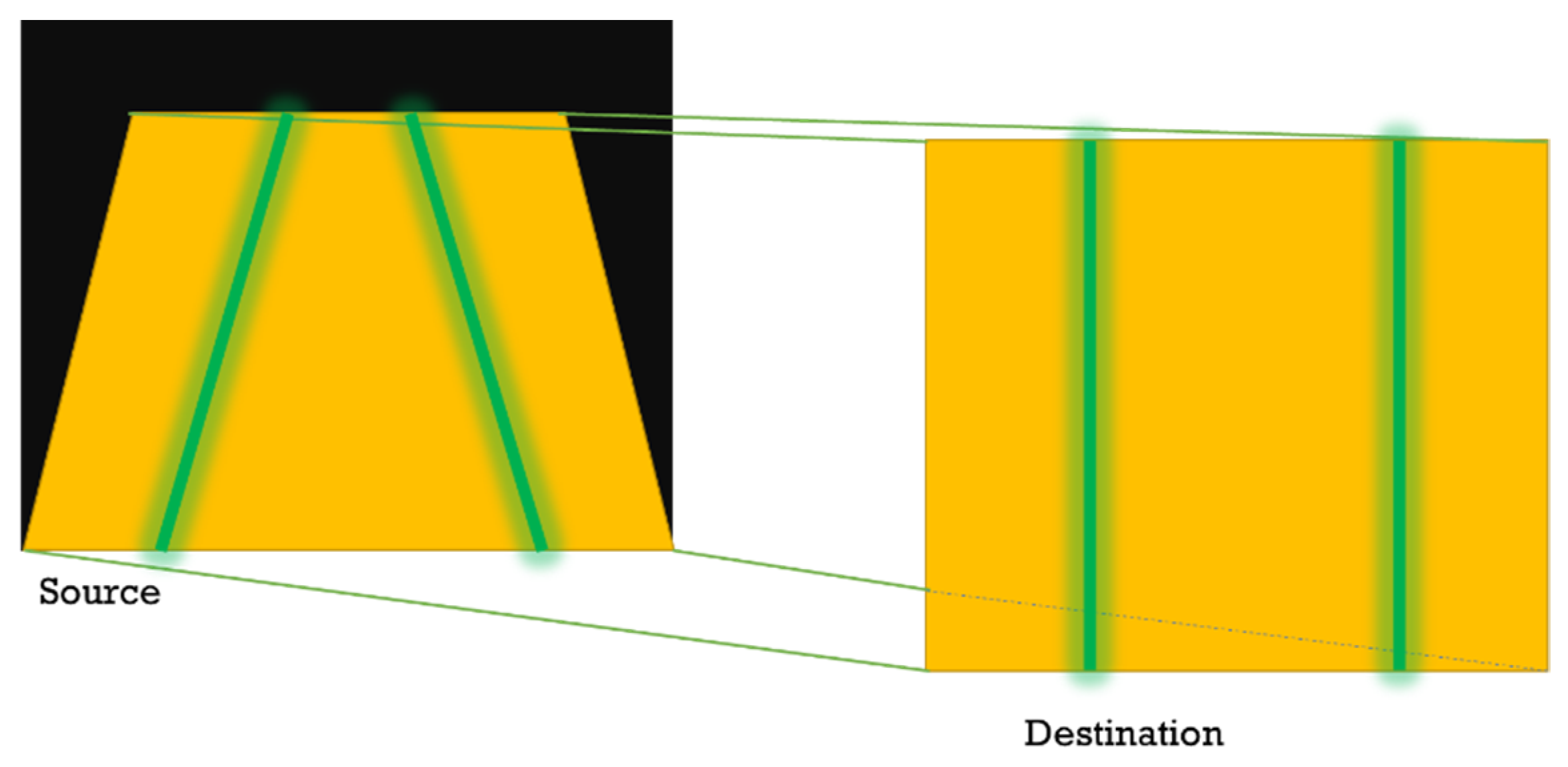
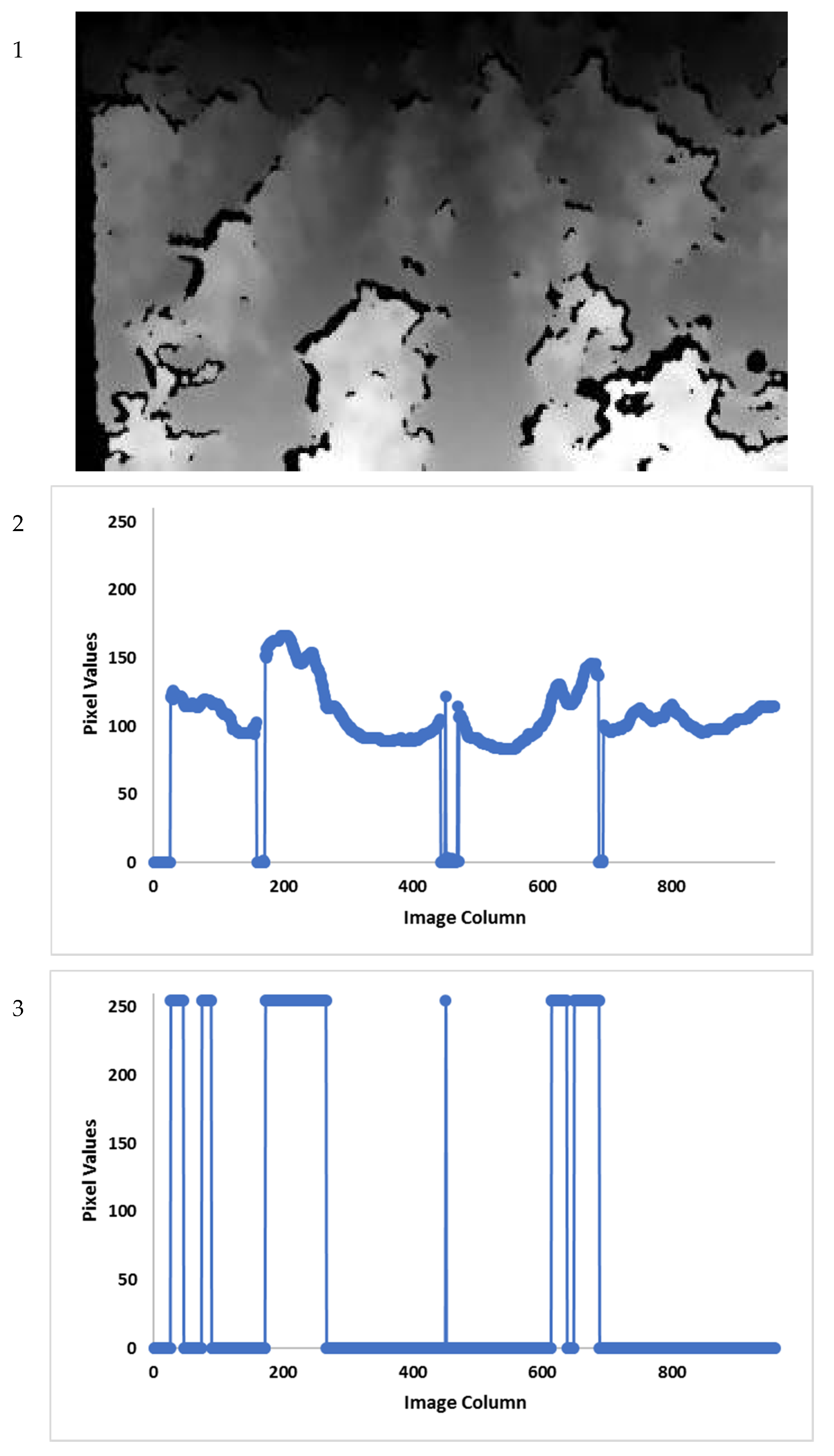
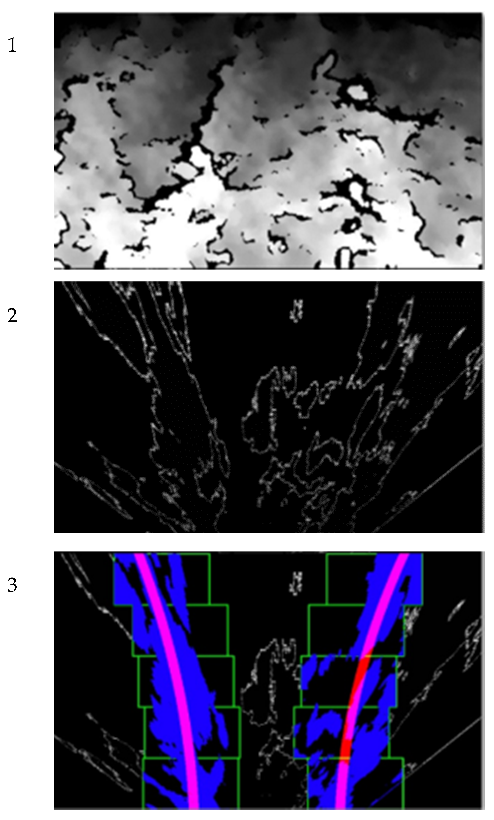
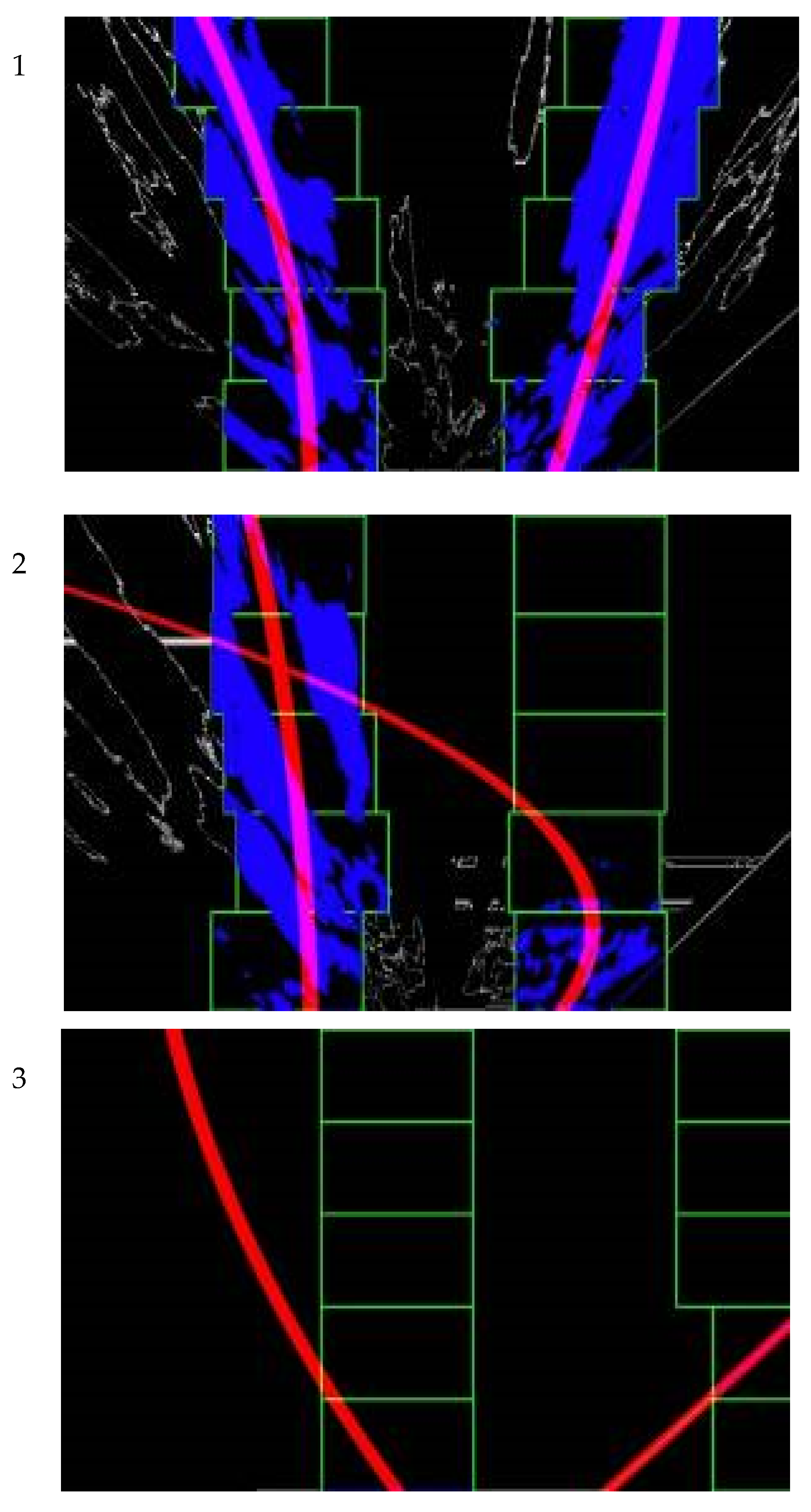
2.2. Cotton Row Detection

Using ZED camera software, the camera was calibrated to achieve the best estimation of the image and real-world coordinates. Calibration of the camera was important since the model would accurately estimate the center of the rover and real-world position of the wheels along the crop rows. The camera parameters cx, cy, fx, fy, k1, and k2 were found. The symbols fx and fy were the focal lengths, cx and cy were the optical center coordinates, both in pixels, and k1 and k2 were distortion parameters used to rectify the images. The ZED SDK performed rectification in the background, and the rectified images were supplied when requested using the ZED application programming interface (API).
  • cx = 674.221
  • cy = 374.301
  • fx = 697.929
  • fy = 697.929
  • k1 = −0.173398
  • k2 = 0.0287331
  • k2 = 0.0287331
[ I x I y 1 ] = [ f x 0 c x 0 0 f y c y 0 0 0 1 0 ] [ W x W y W z 1 ]
where Ix and Iy are image coordinates while Wx, Wy, Wz are real-world coordinates.
The image coordinates can be transformed accurately into real-world coordinates by using the calibrated parameters and Equation (1) above. The images obtained from the left lens of the camera were rectified by balancing and removing distortion. Then, using the right and left lens image, as in Figure 2, the disparity was calculated by the law of registration of the distance between the two lenses and the location of the point targeted [31].
In order to balance the view and determine the row width, it was best to transform the depth map. The transformation was performed by the bird’s eye view model in which it was assumed that the neighboring pixels presented the rows as large, whereas the back ones were small. Hence, the algorithm used the perspective transform to choose a region of interest and transformed it. The transformation was successfully performed on undistorted images. The source image points and destination points in Figure 3 were determined as in Table 1. The transformation vertices were determined experimentally by testing several images and determining camera coverage of the rows.
Because the camera is looking downward, the higher the canopy, the lower the value of the depth. In Figure 4(1), the white pixels represent the upper part of the canopy (high 8-bit values), gray pixels represent the lower part of the canopy, and the soil is represented by black pixels (low 8-bit values). Therefore, in each row of the depth map, these values were determined. The sliding window method was used to determine the depth for each 10 × 10 pixel array by finding the average 8-bit pixel values. The row spacing measurement was determined by connecting all the pixels that were the highest pixel values determined by choosing the 70th percentile of the pixel values. The 70th percentile pixel values provided most of the highest pixel values.
Figure 4 shows the depth map that was manipulated at the center (particularly at the 300th row out of 540 rows of pixels available). The disparity map was 960 pixels wide. Each of the pixels taken was statistically manipulated to get the 70th percentile, which in this case (Figure 4), was 116. Then, all the pixels with the value above 116 were set to white (canopy) and given a value of 255, while all others were reassigned a value of black (value 0). The binary image obtained was further manipulated to more easily delineate crop and row spacing (Figure 4(3)).
Figure 5 presents a depth map that was changed to a binary image, and then transformed to locate the rows; then, the sliding window was used to detect the rows. Figure 5(2) presents a raw depth map. The binary map at the center was obtained by applying the 70th percentile of the row pixels (Figure 5). Then, the sliding window was used to group the pixels and to detect the left and right rows in blue segments. The bottom image in Figure 5 shows the sliding window in green and matching the red line for the left and right row detection. The smooth red line indicates the detection was successful. The algorithm was set such that if the difference between the 90th percentile and the 10th percentile was less than 60, then the whole pixels of the row were converted to black (or zero) because it was not significant to differentiate the top and lower part of the canopy.
The detection was determined as the probability, because it heavily depended on the appearance of the depth map. If the depth map was not uniform with many variations, it was difficult to get a 70th percentile of the pixels that showed uniform changes in the plant canopy. Therefore, a ranking was done (Figure 6) to categorize the detection as good (green), moderate (grey), or no detection (red).
The binary pixels were detected by placing a 100 × 50 pixels window along the left and right row. Then, the points were fitted using a polynomial function to detect the rows. Points were interpolated to find the polynomial function of the second degree. The assumption is that the rows obey the second-degree polynomial function. Assume, (xi,yi) are the distinct points found after matching the pixel sliding window. For distinct points n + 1, x0, x1, x, …, xn−1, xn and corresponding points y0, y1, y2, y3, …, yn−1, and yn; there exists a quadratic equation to fit points [(x0,y0), (x1,y1), (x2,y2), …, (xn−1, yn−1), (xn, yn)]. Assume, function p interpolates pixel values that:
p(xi) = yi for all the values of i from 0, 1, 2, …, n.
For second degree polynomial; then
p ( x i ) = a 2 x i 2 + a 1 x i + a 0 .
Equating Equation (2) and arranging them in matrix form leads to:
[ x 0 2 x 0 1 x 0 2 x 0 1 x 0 2 x 0 1 ] [ a 2 a 1 a 0 ] = [ y 0 y 1 y n ]
The left matrix is called the Vandermonde matrix (V), where a2, a1, and a0 are the coefficients (a) of the predicted polynomial equation that we were required to solve. The Vandermonde matrix is nonsingular.
Va = y
a = V/y
The Manhattan distance between the center of the sliding window and the predicted polynomial fit is calculated to find out how close the sliding window is to the predicted polynomial fit. The points are generated using values of x for each polynomial fit, and then, Manhattan distance is calculated. The distance is expressed as the percentage from the middle of the sliding window to the polynomial fit. Therefore, the polynomial fit should be inside 100% of the sliding window to be determined as the partial detection. If one of the polynomials was greater than 100% offset (Figure 7(3)), it was concluded the row was not detected and marked as a red stripe (Figure 6(3)). When the polynomial fits were 60% or more away from the sliding window (Figure 7(3)), it was concluded to be moderate if there was a row and marked as a gray stripe (Figure 6(2)). When the polynomial fits were 60% or less for both left and right rows from the sliding window (Figure 7(1)), it was concluded that the rows were detected successfully and marked with stripes of yellow and green (Figure 6(1)).

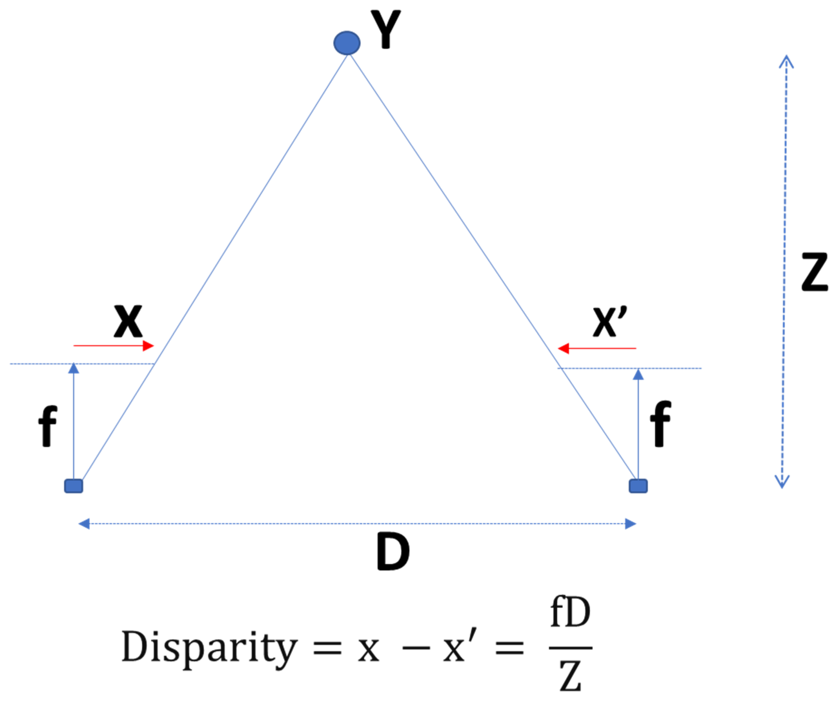
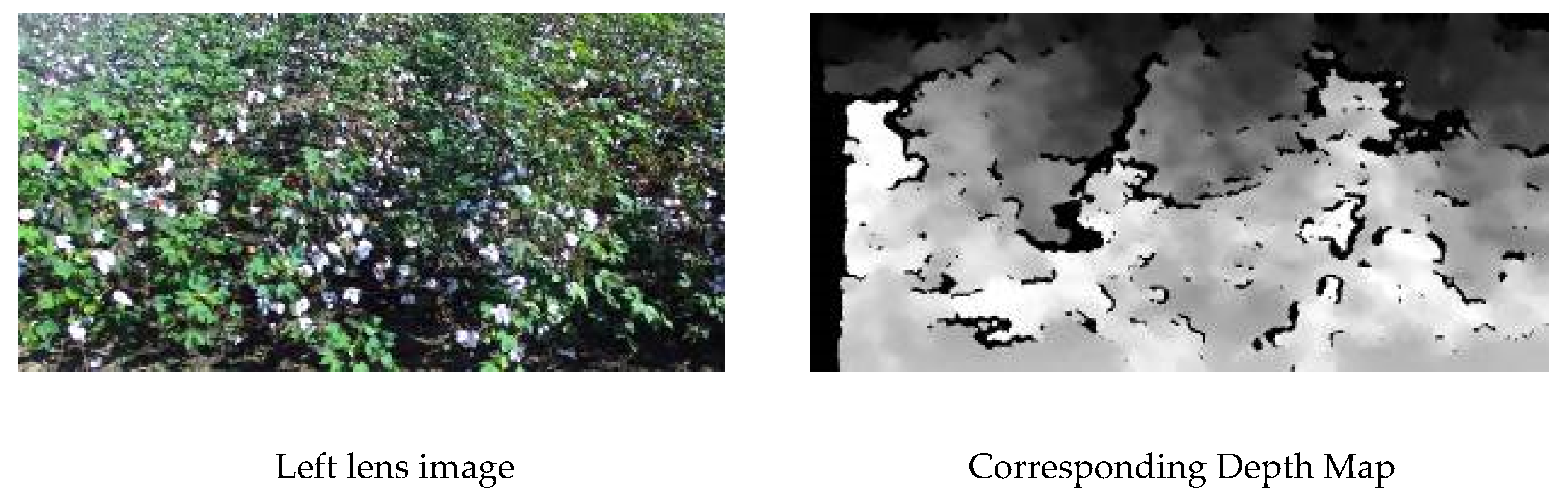
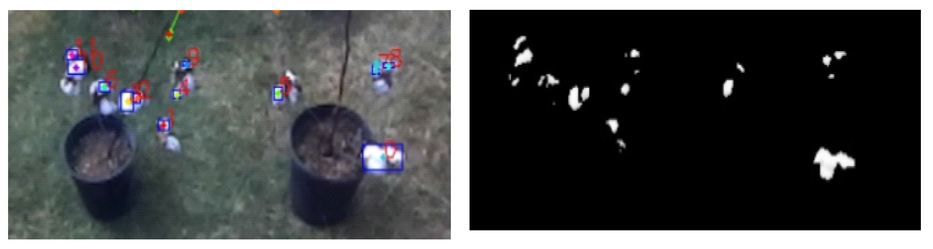
2.3. Boll Detection and Location Estimation

Each image frame was acquired using a ZED camera and analyzed using a 4-step machine vision algorithm (Step 1, depth processing; Step 2, color segmentation; Step 3, feature extraction; and Step 4, frame matching for position determination). These steps were handled by the graphic card optimized rugged development kit (NVIDIA Jetson TX2) to achieve improved matrices calculations using the NVIDIA CUDA cores.
Depth processing was achieved by using the ZED stereo camera, which had two lenses with a separate 1/3″ 4MP CMOS image sensor for each lens. This arrangement allowed the camera to have the ability to process three-dimensional (3D) images that provided the depth measurement of a cotton boll to the camera. The proximity to the cotton bolls was used to determine the distance from the ground, as well as the horizontal distance and vertical distance from the center of the camera carrying platform.
Varying light illumination altered image clarity and boll classification frame-to-frame. In addition, bolls visible to the sensor in one frame became occluded in a subsequent frame of the boll from a different viewpoint of the camera. The boll detection algorithm must have built-in intelligence to remember the last position of the boll even when it appeared undetected in future image frames. Color segmentation was implemented by using machine vision algorithms deployed in the OpenCV library [32]. A machine vision algorithm was required to mask/subtract all background environment and leave cotton bolls in the frame. Since cotton bolls were white, the algorithms, then, needed to mask white objects from the environment. The cotton bolls detection task involved the following four steps [32]:
  • Grab an image;
  • Using the RGB color threshold, separate each RGB component of the image. For cotton bolls, the white components of the image were masked;
  • Subtract the image background from the original image;
  • Remove all the regions where the contours are less than value M. Value M was determined by estimating the number of pixels defining the smallest boll.
The first step was achieved by applying a threshold to separate the white bolls from the background. For white cotton bolls, the color range/threshold was set to 240–255 in the red, green, and blue channel (8-bit color depth map). It made every boll detectable that got proper illumination in at least one image frame. It should be noted that this study is more interested in the depth measurement of the stereo vision system. The second step used feature matching and application of a Boolean “AND” operation between the mask image and the original image. The output image was, then, converted to greyscale.
The last step was feature extraction which was performed by finding contours of consecutive points that had the same intensity and were clustered. Color masking of the grey image was performed, then boundary curves were applied to detect and distinguish all white pixels of the image. For each contour, the center (centroid) was calculated, and the number of pixels that were together was determined. The threshold for the number of pixels together that defined a boll was called M. In this study, two M values, 5 and 15 pixels were chosen and compared.

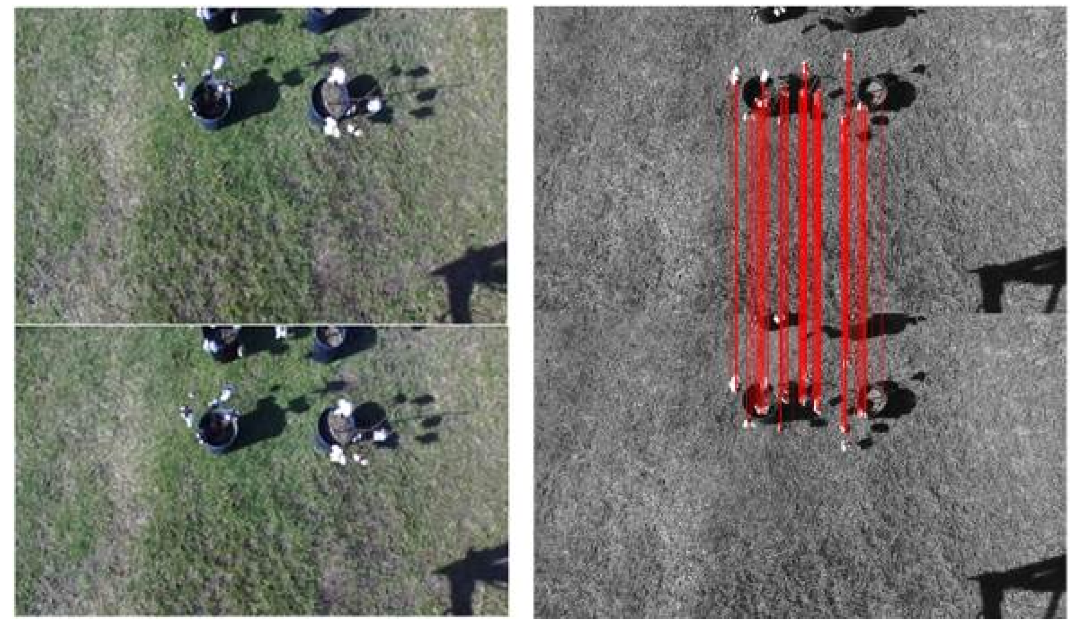
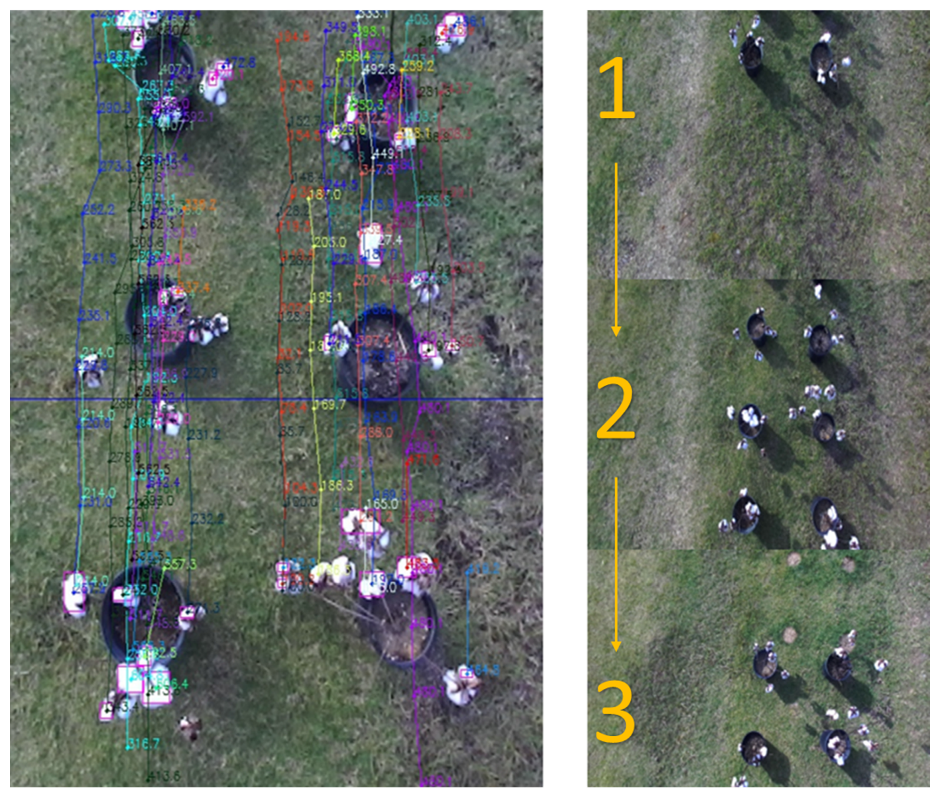
2.4. Frame Feature Extraction, Matching, and Tracking

Frame matching was required to track the position of bolls in respective image frames. In some instances, the algorithm missed the bolls due to illumination problems that impacted brightness, contrast, and sharpness of the image. Hence, the system was developed such that it detected and remembered the boll locations in respective image frames. Since the rover was moving while the bolls were stationary, multiple frames detected bolls with varying depth measurements. Boll tracking was achieved by calculating the projective transformation (homograph) matrix (3 × 3) that matched the point corresponding to two consecutive image frames.
Two consecutive image frames were loaded to the CPU, and the oriented FAST and rotated BRIEF (ORB) feature extraction algorithm was applied to get unique features for both frames to calculate the homograph matrix. The ORB algorithm is a combination of the oriented FAST (features from accelerated segment test) and rotated BRIEF (binary robust independent elementary features) libraries in OpenCV 3.3 [33,34,35]. ORB (an open-source machine vision algorithm) was chosen because it was light and the fastest of all the feature extraction algorithms [34]. The OpenCV Brute force matcher, FLANN matcher, and findHomography modules were used to get the homograph transformation matrix [36]. These algorithms were too slow to achieve the required speed because they were taking more than 4 s to process two images. C++ bytecode that used 8 CUDA threads to utilize the NVIDIA GPU cores was written. The GPU had CUDA cores that deployed fast graphics computing by implementing parallel processing. The C++ bytecode program utilized only 8 of the 256 GPU cores because only two frames were loaded as compared with other applications that deployed a large number of images and hence required more cores. Then, a brute force matcher algorithm that used a random sample consensus (RANSAC) algorithm was written and applied to the images to get the matching features between the images. The RANSAC algorithm interpreted data containing a lot of gross errors, and hence was very useful where several outliers were prevalent [37]. The algorithm used match scores to determine the best matches and left out the outliers [37]. The inliers threshold was determined if at least 5 pixels of the frames matched. Otherwise, it was discarded. By assuming only 20% of the features to match, the system used the RANSAC algorithm to estimate the dataset that contained outliers iteratively (Figure 8).
The RANSAC algorithm followed the following sequence of instructions:
  • A random subset of data was selected, in this case, 20%, and then the model was fitted;
  • The number of outliers was determined, the data was tested against the fitted model, and the points that fitted the model were considered inliers of the consensus set;
  • The program iterated eight times to achieve the best homograph, the number of iterations was determined by the number of CUDA core blocks and threads, and the program established eight threads per block of the CUDA cores;
  • The homograph was, then, parsed by the main program for tracking and logging boll positions.
The overall imaging software was written in Python, but the RANSAC CUDA code was optimized using C++. Then, the Python subprocess code was used to access the CUDA bytecode. With this CUDA optimized implementation, the system was able to process at least two images per second.
Features between two consecutive frames can be projected and located using the homography transformation matrix, as shown in Figure 8. Hence, the new boll position in the next image frame was obtained by multiplying the homography transformation matrix of the initial boll position. For missing bolls in a new image frame, the system used past stored centroids multiplied by the homograph to get the new position of the bolls. After the homograph matrix was obtained, matching boll centroids were determined by using the inverse of the homograph of the current frame and comparing it to the previous image frame. The boll position for each boll was logged and stored as an array.
The rectified image was used to get the z-coordinate (height) of the boll after identifying the bolls. The z-coordinate is the vertical distance of the boll from the ground (height from the ground). It is easy to verify this distance manually to evaluate the sensitivity of the camera. However, a hydraulic on/off directional control valve (DCV) was used to turn the rover, and this sudden change in hydraulic pressure caused a “jerk” in the rover when a turn was initiated, and a subsequent side vibration of the camera resulted, introducing errors and bad rectified image frames. The vision system obtained the rectified left camera images and the corresponding depth maps (disparity image) using an interactive API provided by the camera SDK. The depth map corresponded to a perpendicular distance from the left camera lens to the cotton bolls. Hence, a model was developed to obtain the vertical distance of the boll from the ground. This measurement was the only coordinate that was determined as it is permanent, whereas other readings were relative measurements and changed as the rover moved over the plants. The camera mounted on the rover was inclined at 81.9° from horizontal and obtained 1280 × 720 pixel frames. The field of view was covered at an angle of 54° (Φ) vertically and 96° horizontally.
The system calculated the moving average of cotton boll locations as it grabbed images. The average was used to determine the position of the boll relative to the future cotton-picking end effector. Considering Figure 9, the configuration setup of the rover, camera, and cotton plants is illustrated. Corresponding measurements are as follows:
  • m is the vertical distance from the camera to the cotton bolls;
  • n is the height distance of the boll from the ground;
  • θ is the vertical angle of the object (the cotton boll) from the bottom of the image to the boll;
  • Φ is the vertical field view of the image; and
  • µ is the vertical angle of the image from the bottom of the image to the boll.
The system was developed to measure the distance of the boll from the ground (n). By considering the middle boll (brown arrow), the depth of the boll and distance from the ground was determined. Depth reported by the camera is equal to the one given by the formula m*atan(µ). By using ZED SDK API, the depth of each pixel with a 16-bit resolution was obtained.
Since the camera was inclined at angle µ° from horizontal, the equivalent angle (θ) in radians of the object is given by
a n g l e ( θ ) = π 180 a b s ( ( ( 720 y 720 ) ϕ ) ( 90 µ ɸ / 2 ) ) .
Now, distance from the ground is given by
n = l m atan ( µ ) cos ( θ ) .
Since, depth of an object is provided by ZED SDK then,
n = l d e p t h cos ( θ ) .
The system generated images that showed how the bolls were tracked (Figure 10), and z-coordinate was determined (Equation (7)). The system published images using ROS, and hence clients could get live video of the frames. This video was slower because the system only calculated an average of two frames per second. Graphs were produced to show results.

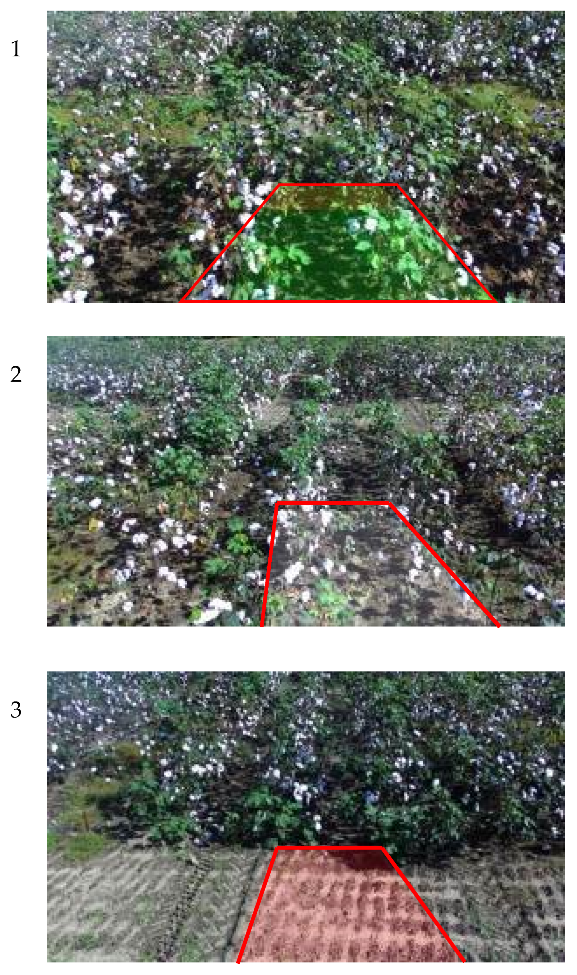
2.5. Data Collection for Row Detection

Field data for row detection were collected at the UGA Lang farm (31.521501, −83.545712) along Carpenter Road, Tifton, GA, USA. The images were collected using the ZED camera at an average frame rate of 5 and a rover speed of 4.8 kph near midday on 28 August 2017. The images and depth maps were stored in the internal memory of the development kit. A total of 381 of the collected images (images such as Figure 11) that cover four rows passing the first two, and then the next two rows when coming back were used for analysis and validation of the row detection model.

2.6. Data Collection for Boll Detection and Position Estimation

In December 2017, an experiment, to evaluate the cotton boll tracking model, was conducted at the UGA campus grounds (N Entomology Dr, Tifton, GA, USA, 31793) at (31°28′ N, 83°31′ W). The location was open to direct sunlight. Twelve defoliated cotton plants were taken from a nearby farm and put in soil-filled pots. The plants were placed in 2 rows of 6 plants. The plants were 91.4 cm between the center of the stalk (row spacing) and each stalk was 61 cm from the next (plant spacing). The distances of all bolls were measured manually, and the rover was driven over the bolls collecting RGB and depth information from the ZED camera. A static test was first conducted on 1 December 2017 with the rover set over the bolls, and two consecutive frames were taken.
The second test was conducted on 4 December 2017. The plants were randomized, and data collected in three rover speed treatments, 1.04 km/h, 0.80 km/h, and 0.64 km/h. The relative positions of the bolls were determined by measuring boll distance from the ground. The data were collected by changing the M parameter (from 15 to 5) to detect white contours (cotton bolls). A comparison of the camera and manual measurement of boll locations was conducted. Comparative statistics were used to measure standard error, root mean square error, and mean error.

3. Results and Discussions

3.1. Row Detection

The 381 images collected were each evaluated to assess the detection of the rows (Table 2). Results were based on the ranking of the software, as previously described, to determine if row detection was successful. Images were manually categorized as difficult or easy. The easy detection categorization meant the software detection was correct since the canopies were explicitly separated, and rows could easily be seen, and hence, all the rows aligned with a sliding window. Difficult categorization meant the image had plant canopies heavily overlapping to each other, which made it difficult to differentiate the two rows, and hence, some of the row pixels were out of the sliding window, but the detection was still successful. The true positive categorization meant the row detection was successful. The false Positive categorization meant row detection was found in a place where there were no visible rows. False positives occurred when plants other than cotton appeared between rows, or the depth image obtained was blurred. True negative meant rows were not detected, and the software successfully assigned no rows to that situation. The easy category meant the system was 100% sure there were no rows because there were no differences between upper pixels and lowers pixels, confirming the absence of a plant canopy. False negatives were situations where the software did not detect a row when a row was there. It was most commonly caused by skips in the rows where cotton was not growing.
precision = TP / ( TP + FP ) = 283 / 284 = 0.996
recall = TP / ( TP + FN ) = 283 / ( 283 + 28 ) = 0.909
F 1   Score = 2 Precision recall precision + recall = 0.951
Accuracy = ( TP + TN ) / ( TP + FP + FN + TN ) = ( 283 + 69 ) / 381 = 0.923
The model was evaluated from the data collected (Table 2). The vision system was found to perform at 92.3% accuracy with an F1 score of 0.951. The algorithm was accurate, but it had many difficulties in predicting the rows that had plants that were shorter or taller than the average cotton plant. Some rows were occluded by plants from both sides of the row that had a big canopy that fully occupied the row. These situations led to the row detection algorithm predicting 28 false negatives cases.

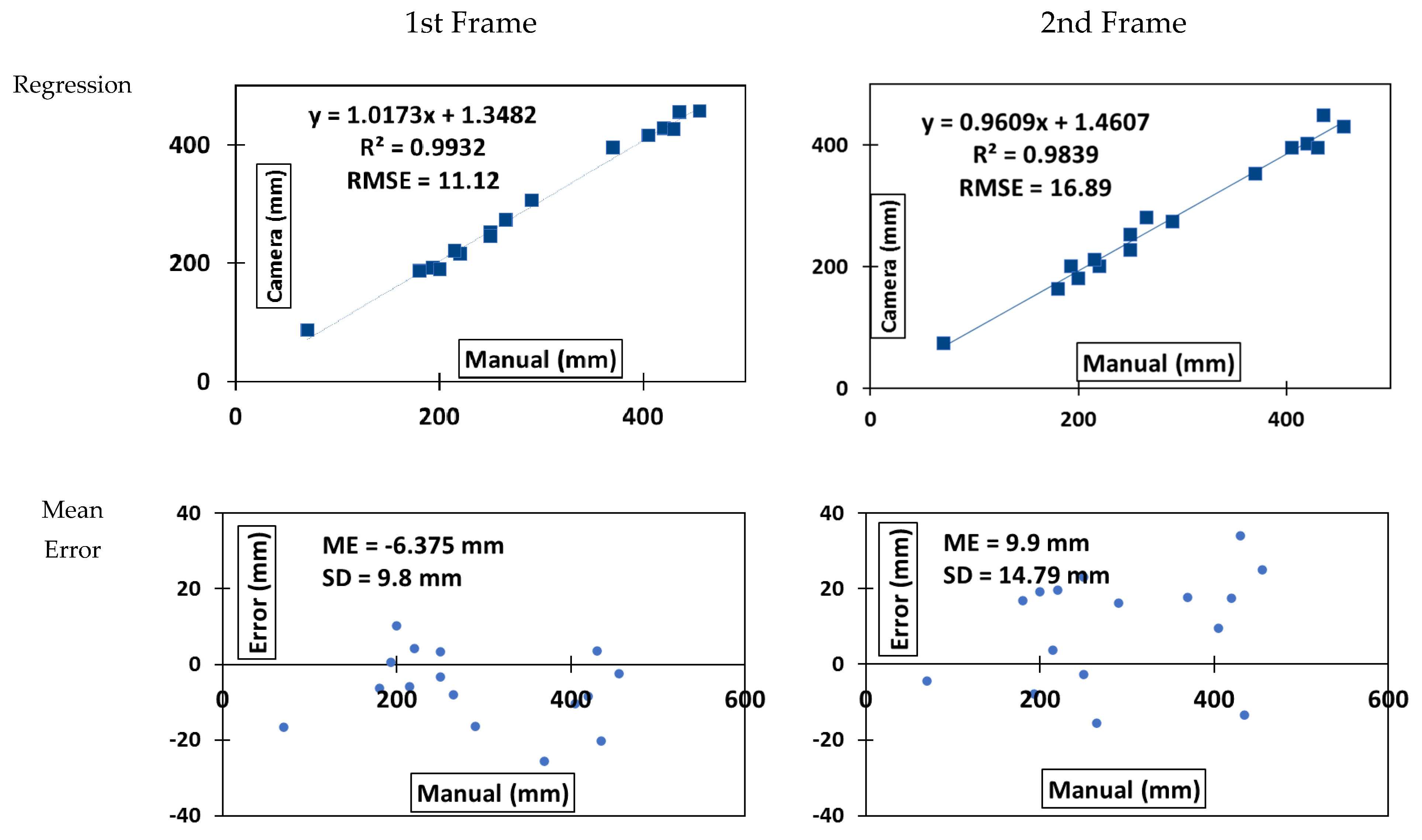
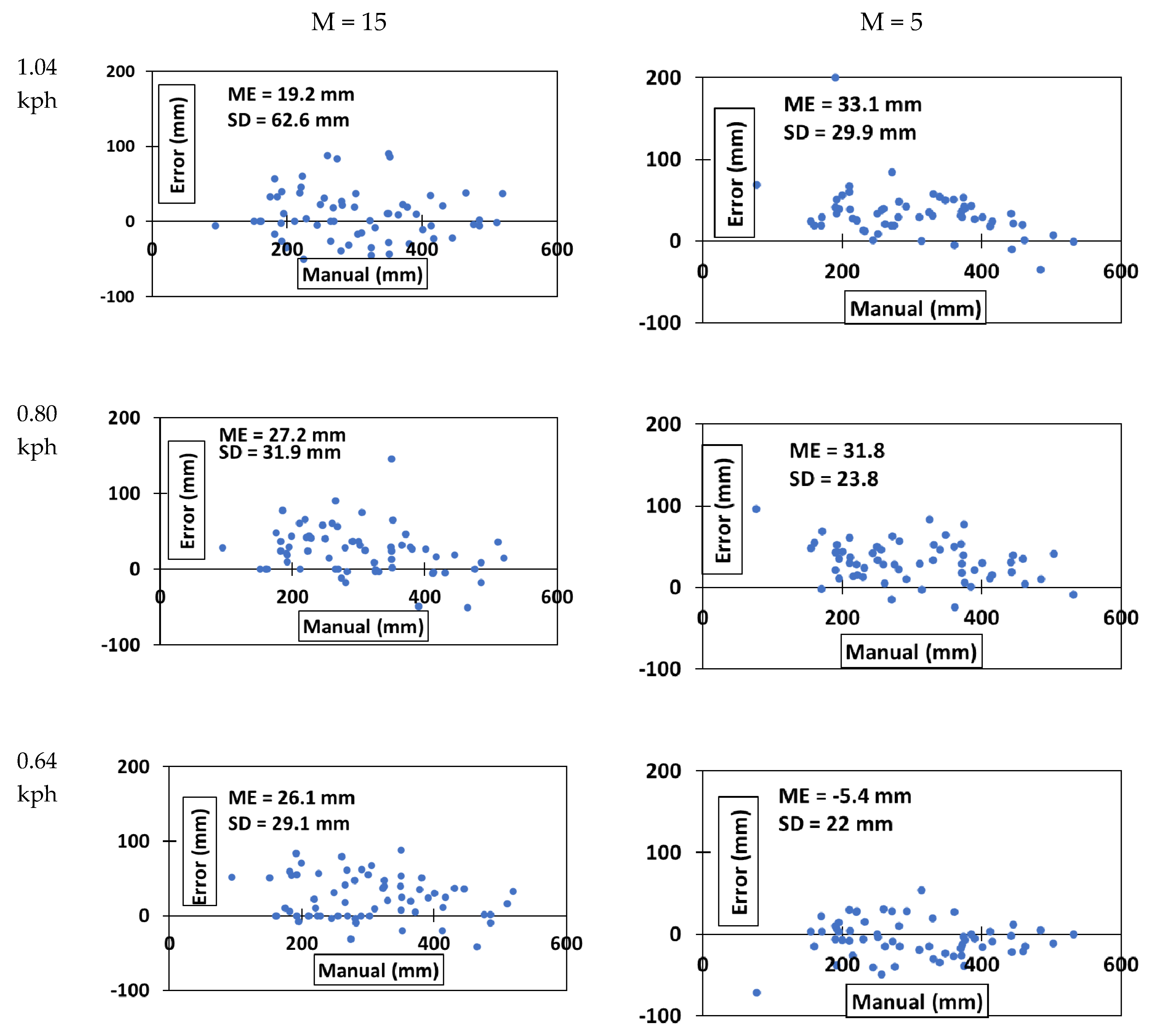
3.2. Cotton Boll Detection and Position Estimation

A static test was conducted to assess the ability of the camera to classify and locate bolls without the dynamics of a moving camera. The red rover was set stationary but running, and two consecutive frames were collected second and analyzed (Figure 12). Using Excel, the manual measurements of sixteen boll locations were compared to camera image measurements. The camera accuracy from the first image frame showed a regression relationship to the manual measurements of R2 equal to 99% and a root mean square error (RMSE) of 11 mm. The second frame gave R2 equal to 98%, and a RMSE of 17 mm. The mean errors were −6 mm and 9.9 mm for first and second frames, respectively. The standard deviations were 9.8 mm and 14.8 mm for the first and second frames, respectively (Figure 12). The results show that the camera system was able to classify and locate bolls under direct sunlight with low cotton boll density.
The software detected the bolls and recorded multiple depths for the same boll as the vehicle moved over the row during the test. The 15 pixel boll contour (M = 15) was only able to detect 92.3% of all 65 bolls available, whereas, when M = 5 was introduced, the system was able to detect all the bolls. Figure 13 demonstrates the results of color segmentation detection and masking. The white spaces had to form a contour that passed the threshold M value, 15 or 5 pixels. The color of the boll and obstruction could make one boll detectible in one frame but not the next. The same boll could also be detected in consecutive frames. By being detected more than once, the system was able to obtain more than one depth reading for individual bolls. Multiple values obtained were averaged to get an estimated depth value. Figure 14 shows the regression relationship of the experiment for all three different speed tests. Figure 15 shows the mean error distribution of the experiment. The boll detection algorithm had the worst R2 of 0.86 for the highest rover speed (1.04 kph) and M = 15 contour, while R2 of 0.95 for the slowest rover speed (0.64 kph) M = 5 contour. In Figure 15, results showed that the M = 15 data had a larger RMSE as compared with M = 5. These errors were mainly due to the “jerking” of the rover when adjusting the right and left turn and topography of the land to maintain a straight path for the rover.

4. Conclusions

Imaging systems to determine 3D boll location and row detection were developed and evaluated in this study. The performance of the algorithm developed in this study to detect the rows showed promise as a method to assist with the RTK-GNSS navigation of an intelligent rover for harvesting cotton bolls. Adding a visual system to the navigation provided an increased perception of the environment to aid in avoiding obstacles and seeing the actual row path for the vehicle. Furthermore, in the case of failures of the RTK-GNSS, the camera system can help the rover to continue moving without pausing to regain localization, which can cost field operational time. The results suggest that the visual system can be deployed for rover navigation assistance and replacement during GNSS interruptions. However, the visual system only works looking downward when rows are not occluded with large plant canopies or in places with no plants. A camera closer to the ground positioned horizontally or slightly upward into the canopy could provide a better perspective of rows closer to the plant crown at the ground.
For the boll location, the system was able to acquire images and process two frames per second using the GPU resources of the system. When comparing the boll detection and localizing system to the manual measurements, the performance was proportional to the speed of the rover and contour threshold (M) used to detect bolls with better performance. With M = 5, the system detects multiple contours for the same boll as compared with M = 15. As a result, the boll tracking system decreases time spent errantly tracking multiple contours as different bolls, when there is only one boll present. It should help to increase harvest speed when using a robotic arm with an end effector to harvest cotton bolls identified by the boll tracking system. The results showed that the rover would have to stop in some locations to get the best measurement of boll locations in the field for cotton boll picking with a robotic arm. The accuracy achieved by tracking cotton bolls is favorable for proceeding to the development of a cotton harvesting robot. Future research should involve more field testing of the models developed in this study, in realistic conditions.

Author Contributions

Conceptualization, K.F., and G.R.; methodology, K.F., and G.R.; formal analysis, K.F.; software, K.F.; writing—original draft preparation, K.F.; writing—review and editing, K.F., W.P., C.L., and G.R.; supervision, C.L. and G.R.; project administration, W.P., E.B., and G.R. All authors have read and agreed to the published version of the manuscript.

Funding

This research was funded by COTTON INCORPORATED, Agency Assignment Number 17-038.

Acknowledgments

The authors are very thankful for project support from Cotton Incorporated, Agency Assignment #17-038. We also thank Ricky Fletcher and Gary Burnham for their helpfulness and technical support in building the camera platform and collection of data.

Conflicts of Interest

The authors declare no conflict of interest.

Nomenclature

RTK-GNSSReal-Time Kinematic Global Navigation Satellite System
OpenCVOpen Computer Vision Library
CUDACompute Unified Device Architecture
ROSRobot operating system
SDKSoftware development kit
3DThree-dimensional
2DTwo-dimensional
HzHeitz
FASTFeatures from accelerated segment test
BRIEFBinary robust independent elementary features
ORBOriented FAST and rotated BRIEF
RANSACRandom sample consensus
FLANNFast Library for Approximate Nearest Neighbors
RMSERoot mean square error
RGBRed-green-blue
ARMAdvanced RISC machine
HMPHeterogeneous multiprocessing
LPDDRLow-Power Double Data Rate Synchronous Dynamic Random-Access Memory
eMMCEmbedded multimedia card
SATASerial AT attachment
DCVDirectional control valve
APIApplication programming interface
UGAUniversity of Georgia

References

  1. Fue, K.G.; Porter, W.M.; Barnes, E.M.; Rains, G.C. An Extensive Review of Mobile Agricultural Robotics for Field Operations: Focus on Cotton Harvesting. AgriEngineering 2020, 2, 10. [Google Scholar] [CrossRef] [Green Version]
  2. Kise, M.; Zhang, Q.; Más, F.R. A stereovision-based crop row detection method for tractor-automated guidance. Biosyst. Eng. 2005, 90, 357–367. [Google Scholar] [CrossRef]
  3. Hayes, L. Those Cotton Picking Robots. Available online: http://georgia.growingamerica.com/features/2017/08/those-cotton-picking-robots/ (accessed on 19 December 2017).
  4. Romeo, J.; Pajares, G.; Montalvo, M.; Guerrero, J.M.; Guijarro, M.; Ribeiro, A. Crop row detection in maize fields inspired on the human visual perception. Sci. World J. 2012, 2012. [Google Scholar] [CrossRef] [Green Version]
  5. Winterhalter, W.; Fleckenstein, F.V.; Dornhege, C.; Burgard, W. Crop row detection on tiny plants with the pattern hough transform. IEEE Robot. Autom. Lett. 2018, 3, 3394–3401. [Google Scholar] [CrossRef]
  6. Rains, G.C.; Bazemore, B.W.; Ahlin, K.; Hu, A.-P.; Sadegh, N.; McMurray, G. Steps towards an Autonomous Field Scout and Sampling System. In Proceedings of the 2015 ASABE Annual International Meeting, New Orleans, LA, USA, 26–29 July 2015. [Google Scholar] [CrossRef]
  7. Rains, G.C.; Faircloth, A.G.; Thai, C.; Raper, R.L. Evaluation of a simple pure pursuit path-following algorithm for an autonomous, articulated-steer vehicle. Appl. Eng. Agric. 2014, 30, 367–374. [Google Scholar]
  8. Van Henten, E.J.; Van Tuijl, B.A.J.; Hemming, J.; Kornet, J.G.; Bontsema, J.; Van Os, E.A. Field Test of an Autonomous Cucumber Picking Robot. Biosyst. Eng. 2003, 86, 305–313. [Google Scholar] [CrossRef]
  9. Kondo, N. Study on grape harvesting robot. IFAC Proc. Vol. 1991, 24, 243–246. [Google Scholar] [CrossRef]
  10. Luo, L.; Tang, Y.; Zou, X.; Ye, M.; Feng, W.; Li, G. Vision-based extraction of spatial information in grape clusters for harvesting robots. Biosyst. Eng. 2016, 151, 90–104. [Google Scholar] [CrossRef]
  11. Li, J.; Karkee, M.; Zhang, Q.; Xiao, K.; Feng, T. Characterizing apple picking patterns for robotic harvesting. Comput. Electron. Agric. 2016, 127, 633–640. [Google Scholar] [CrossRef] [Green Version]
  12. Zhao, Y.; Gong, L.; Huang, Y.; Liu, C. Robust tomato recognition for robotic harvesting using feature images fusion. Sensors 2016, 16, 173. [Google Scholar] [CrossRef] [PubMed] [Green Version]
  13. Hayashi, S.; Yamamoto, S.; Saito, S.; Ochiai, Y.; Kamata, J.; Kurita, M.; Yamamoto, K. Field operation of a movable strawberry-harvesting robot using a travel platform. Jpn. Agric. Res. Q. JARQ 2014, 48, 307–316. [Google Scholar] [CrossRef] [Green Version]
  14. Williams, H.A.M.; Jones, M.H.; Nejati, M.; Seabright, M.J.; Bell, J.; Penhall, N.D.; Barnett, J.J.; Duke, M.D.; Scarfe, A.J.; Ahn, H.S. Robotic kiwifruit harvesting using machine vision, convolutional neural networks, and robotic arms. Biosyst. Eng. 2019, 181, 140–156. [Google Scholar] [CrossRef]
  15. Bac, C.W.; Hemming, J.; van Tuijl, B.A.J.; Barth, R.; Wais, E.; van Henten, E.J. Performance Evaluation of a Harvesting Robot for Sweet Pepper. J. Field Robot. 2017, 34, 1123–1139. [Google Scholar] [CrossRef]
  16. Arad, B.; Balendonck, J.; Barth, R.; Ben-Shahar, O.; Edan, Y.; Hellström, T.; Hemming, J.; Kurtser, P.; Ringdahl, O.; Tielen, T. Development of a sweet pepper harvesting robot. J. Field Robot. 2020. [Google Scholar] [CrossRef]
  17. Zion, B.; Mann, M.; Levin, D.; Shilo, A.; Rubinstein, D.; Shmulevich, I. Harvest-order planning for a multiarm robotic harvester. Comput. Electron. Agric. 2014, 103, 75–81. [Google Scholar] [CrossRef]
  18. Rovira-Más, F.; Zhang, Q.; Reid, J.; Will, J. Hough-transform-based vision algorithm for crop row detection of an automated agricultural vehicle. J. Auto. Eng. 2005, 219, 999–1010. [Google Scholar] [CrossRef]
  19. García-Santillán, I.; Guerrero, J.M.; Montalvo, M.; Pajares, G. Curved and straight crop row detection by accumulation of green pixels from images in maize fields. Precis. Agric. 2018, 19, 18–41. [Google Scholar] [CrossRef]
  20. Zhai, Z.; Zhu, Z.; Du, Y.; Song, Z.; Mao, E. Multi-crop-row detection algorithm based on binocular vision. Biosyst. Eng. 2016, 150, 89–103. [Google Scholar] [CrossRef]
  21. UGA. Georgia cotton production guide. In Ugacotton Org; Team, U.E., Ed.; UGA Extension Team: Tifton, Switzerland, 2019. [Google Scholar]
  22. Higuti, V.A.H.; Velasquez, A.E.B.; Magalhaes, D.V.; Becker, M.; Chowdhary, G. Under canopy light detection and ranging-based autonomous navigation. J. Field Robot. 2019, 36, 547–567. [Google Scholar] [CrossRef]
  23. Bulanon, D.M.; Kataoka, T.; Okamoto, H.; Hata, S.-I. Development of a real-time machine vision system for the apple harvesting robot. In Proceedings of the SICE 2004 Annual Conference, Sapporo, Japan, 4–6 August 2004; pp. 595–598. [Google Scholar]
  24. Jiang, Y.; Li, C.; Paterson, A.H. High throughput phenotyping of cotton plant height using depth images under field conditions. Comput. Electron. Agric. 2016, 130, 57–68. [Google Scholar] [CrossRef]
  25. Wang, Y.; Zhu, X.; Ji, C. Machine Vision Based Cotton Recognition for Cotton Harvesting Robot. In Proceedings of the Computer and Computing Technologies in Agriculture, Boston, MA, USA, 18–20 October 2008; pp. 1421–1425. [Google Scholar]
  26. Mulan, W.; Jieding, W.; Jianning, Y.; Kaiyun, X. A research for intelligent cotton picking robot based on machine vision. In Proceedings of the 2008 International Conference on Information and Automation, Changsha, China, 20–23 June 2008; pp. 800–803. [Google Scholar]
  27. Xu, S.; Wu, J.; Zhu, L.; Li, W.; Wang, Y.; Wang, N. A novel monocular visual navigation method for cotton-picking robot based on horizontal spline segmentation. In Proceedings of the MIPPR 2015 Automatic Target Recognition and Navigation, Enshi, China, 31 October–1 November 2015; p. 98121B. [Google Scholar]
  28. Rao, U.S.N. Design of automatic cotton picking robot with Machine vision using Image Processing algorithms. In Proceedings of the 2013 International Conference on Control, Automation, Robotics and Embedded Systems (CARE), Jabalpur, MP, India, 16–18 December 2013; pp. 1–5. [Google Scholar]
  29. Lumelsky, V. Continuous motion planning in unknown environment for a 3D cartesian robot arm. In Proceedings of the 1986 IEEE International Conference on Robotics and Automation, San Fransisco, CA, USA, 7–10 April 1986; pp. 1050–1055. [Google Scholar]
  30. Zefran, M. Continuous Methods for Motion Planning. Ph.D. Thesis, University of Pennsylvania, Philadelphia, Pennsylvania, December 1996. Available online: http://repository.upenn.edu/ircs_reports/111 (accessed on 12 June 2019).
  31. Lucas, B.D.; Kanade, T. An iterative image registration technique with an application to stereo vision. In Proceedings of the 7th International Joint Conference on Artificial Intelligence, San Francisco, CA, USA, 24–28 August 1981; pp. 674–679. [Google Scholar]
  32. Gong, Y.; Sakauchi, M. Detection of regions matching specified chromatic features. Comput.Vis. Image Under. 1995, 61, 263–269. [Google Scholar] [CrossRef]
  33. Calonder, M.; Lepetit, V.; Strecha, C.; Fua, P. Brief: Binary robust independent elementary features. In Proceedings of the 11th European Conference on Computer Vision, Crete, Greece, 5–11 September 2010; pp. 778–792. [Google Scholar]
  34. Rublee, E.; Rabaud, V.; Konolige, K.; Bradski, G. ORB: An efficient alternative to SIFT or SURF. In Proceedings of the 2011 International Conference on Computer Vision, Barcelona, Spain, 6–13 November 2011; pp. 2564–2571. [Google Scholar]
  35. Rosten, E.; Drummond, T. Machine learning for high-speed corner detection. In Proceedings of the 9th European Conference on Computer Vision, Graz, Austria, 7–13 May 2006; pp. 430–443. [Google Scholar]
  36. Muja, M.; Lowe, D.G. Scalable Nearest Neighbor Algorithms for High Dimensional Data. IEEE Trans. PAMI 2014, 36, 2227–2240. [Google Scholar] [CrossRef] [PubMed]
  37. Fischler, M.A.; Bolles, R.C. Random sample consensus: A paradigm for model fitting with applications to image analysis and automated cartography. Commun. ACM 1981, 24, 381–395. [Google Scholar] [CrossRef]
Figure 1. Machine vision components of the research.
Agronomy 10 01137 g001
Figure 2. Disparity calculation. Where x and x’ are the distance between points in the image plane corresponding to the three-dimensional (3D) scene point and their camera center. D is the distance between two lenses of the stereo camera, and f is the focal length of both lenses. Y is the location of the object, whereas Z is the distance of the object to the camera.
Agronomy 10 01137 g002
Figure 3. The perspective transformation of the depth maps. The rows are transformed using the equations in Table 1 to generate a map that shows the rows to approximately straight rows that would allow an algorithm to detect the rows easily.
Agronomy 10 01137 g003
Figure 4. Depth map at the row pixel number 300 (each image has 540 row of pixels) (1); The pixels are captured in the histogram (2); and then using the 70th percentile only pixels with a value above 116 are used to form a binary image histogram (3).
Agronomy 10 01137 g004
Figure 5. Rows are detected by using depth map (1); transformed binary depth map at the center (2); while lower image (3) represents the sliding window detection of the rows.
Agronomy 10 01137 g005
Figure 6. Ranking the detection of the rows (the upper image means detection is successful as it shows green and yellow stripes, center image detection with gray stripe is moderately successful, and the bottom with red stripe means no rows are detected).
Agronomy 10 01137 g006
Figure 7. Sliding window comparison with the polynomial fit using Manhattan distance. The upper image (1) was successful detection; center image detection (2) was moderate detection; and the lower image (3) indicated no row detection.
Agronomy 10 01137 g007
Figure 8. Two consecutive images collected from the ZED camera and the moving rover (left images) and matching features obtained using the oriented FAST and rotated BRIEF (ORB) algorithm and the homograph random sample consensus (RANSAC) algorithm (right image).
Agronomy 10 01137 g008
Figure 9. Context diagram that shows cotton boll position measurements.
Agronomy 10 01137 g009
Figure 10. Left image shows processed boll position and tracking of the boll while the right images show a series of 3 image frames acquired from the moving camera.
Agronomy 10 01137 g010
Figure 11. Collected RGB image and corresponding depth map for cotton row detection (0–255, 8-bit greyscale image).
Agronomy 10 01137 g011
Figure 12. Comparison of the image frames when the rover was stationary. The y-axis is the camera measurements, while the x-axis is the manual measurements. the first and second frames were taken consecutively to compare the depth estimation.
Agronomy 10 01137 g012
Figure 13. Segmentation results and masking of the images.
Agronomy 10 01137 g013
Figure 14. Comparison of 15 pixels contour and 5 pixels contour for 1.04 kph (fast speed), 0.80 kph (slow speed), and 0.64 kph (very slow speed) of cotton boll position measurements.
Agronomy 10 01137 g014
Figure 15. The mean error distribution of the experiment (M = 5) and the 15 pixel contour for 1.04 kph (fast speed), 0.80 kph (slow speed), and 0.64 mph (very slow speed) of cotton boll position measurements).
Agronomy 10 01137 g015
Table 1. The perspective transformation vertices for depth maps. Part of the source image vertices are chosen, and then transformed into another image (destination) that can easily show the rows in straight patterns, which can easily let the model detect the shape of the rows. The width of the image was 960 pixels, and the height was 540 pixels. The ratios times the width or height provide the vertices for the destination images.
Source Image Points (Vertices)Destination Image Points (Vertices)
0.65 × 960, 0.65 × 540960 × 0.75
960, 540960 × 0.75, 540
0, 540960 × 0.25, 540
0.40 × 960, 0.40 × 540960 × 0.25
Table 2. Results of the manual inspection of the images.
EasyDifficultTotal
True Positive20776283
False Positive000101
True Negative541569
False Negative052328
Total266115381

