Pear Flower Cluster Quantification Using RGB Drone Imagery

Abstract

High quality fruit production requires the regulation of the crop load on fruit trees by reducing the number of flowers and fruitlets early in the growing season, if the bearing is too high. Several automated flower cluster quantification methods based on proximal and remote imagery methods have been proposed to estimate flower cluster numbers, but their overall performance is still far from satisfactory. For other methods, the performance of the method to estimate flower clusters within a tree is unknown since they were only tested on images from one perspective. One of the main reported bottlenecks is the presence of occluded flowers due to limitations of the top-view perspective of the platform-sensor combinations. In order to tackle this problem, the multi-view perspective from the Red–Green–Blue (RGB) colored dense point clouds retrieved from drone imagery are compared and evaluated against the field-based flower cluster number per tree. Experimental results obtained on a dataset of two pear tree orchards (N = 144) demonstrate that our 3D object-based method, a combination of pixel-based classification with the stochastic gradient boosting algorithm and density-based clustering (DBSCAN), significantly outperforms the state-of-the-art in flower cluster estimations from the 2D top-view (R² = 0.53), with R² > 0.7 and RRMSE < 15%.

1. Introduction

In fruit orchards, spatial explicit flowering information is key in guiding the processes of pruning of branches and flower thinning, which directly impact crop load, fruit size, coloration, and taste. Visual flower counting is currently the most common approach for bloom intensity estimation in orchards, but is a technique which is time consuming, labor-intensive and prone to errors if not done by experts. Since only a limited sample of the trees is inspected, extrapolation to the entire orchard relies strongly on the grower’s experience as no information on the spatial variability within the orchards is provided [1,2,3]. These limitations, in combination with the short-term nature of flower appearance, make an automated method highly desirable. Imaging methods ranging from spaceborne to proximal platforms can deliver the inputs needed to automate flower mapping. However, existing satellite flower mapping methods are mainly focused on the detection of the onset of flowering in trees but are usually too coarse (>10 m) to accurately determine the flower number [4,5]. Flower number mapping with manned airborne platforms is feasible but demands more expensive sensors with a higher spectral resolution to compensate for the lack in spatial resolution [6,7]. Therefore, due to the size of the flowers (<2 cm) and flower clusters (i.e., a group of seven to nine pear flowers <120 cm²), highly spatially detailed images from proximal sensors are preferred for flower quantification. The application of drones is usually preferred over a ground vehicle or robot to collect this data, as a drone can provide superior data collection speed and larger spatial coverage. In addition, drones do not interact with the plants, so constant data collection will not cause soil compaction and plant damage, which can happen when using a ground vehicle [8].

To the best of our knowledge, previous studies using proximal data for flower detection and classification, only focused on Red–Green–Blue (RGB) and multispectral sensors [8,9,10,11,12]. As flowers generally have a distinct color from the background, the three or four bands of these sensors suffice for distinguishing the flowers from the rest of the orchard scene. The number of flowers can be estimated by either pixel-based or object-based classification methods [13]. Most common pixel-based methods for flower classification are simple thresholding techniques [9,10,11,14,15,16], where images are segmented by a binary partitioning of the image intensities with a given threshold [17]. Although popular, these methods are hindered by variable lighting conditions and thus manual threshold adjustment for new data is needed. Other researchers used more advanced machine and deep learning techniques such as support vector machines [18,19], random forests [19], K-means [16] and convolutional neural networks (CNN) [12] which are more robust pixel-based flower classification methods. Once flower pixels are identified, flower numbers are estimated via flower pixel amount or fraction [9,16]. The problem with this methodology is that it assumes that flowers or flower clusters always have the same size. This is not the case since they can differ in size due to occlusion by the canopy [16], the phenological stage they are in [8] and differences in scale due to the position of the flowers on the tree along the z-axis. In contrast to pixel-based methods, object-based classification methods first aggregate spectrally homogenous image objects using an image segmentation algorithm, followed by a classification of the individual objects [13]. This object-based classification can be performed in multiple steps with the use of morphological operations on the individual classified flower pixels [19,20,21] or by direct object-based CNN [8]. The latter will evaluate directly if a small image patch contains a flower or not without a need for a pixel-based classification step [8,22].

When evaluating flower counting methods, different approaches have been used. An important aspect is the focus of the research, which could be (1) how well the flowers which are present in an image can be detected and counted (i.e., image-based flower clusters), and (2) how well the flowers which are present in a tree (i.e., field-based flower clusters) can be detected and counted. The former focusses on the classification accuracy, which has been the main objective of most of the existing literature. The latter is often a combination of different factors, including the classification accuracy, but also the extent to which all flowers from the tree are visible/detectable in the image. Examples of the first are the pixel-wise classification accuracy [18,23] or the accuracy based on flowers which can be seen on the imagery [12]. However, for the end-user of the flower maps the second is more important and to our knowledge, only Hočevar (2014) [10] and Tubau et al. (2019) [16] have reported the correlation between their flower estimations and the real number of flowers, giving respectively a R² of 0.59 and 0.56 for apple trees. The first, reaching the highest accuracy, used one-side perspective imagery per tree, while the second used the top-view perspective for each tree to estimate flower numbers. Therefore, for the second evaluation method aside from sensor-platform system and classification algorithm, the viewing perspective on the tree also determines the accuracy of the flower counting method. The viewing perspective should guarantee that all flowers which are present on the tree can be counted. Unfortunately, most studies only include a uni-perspective view, namely the side-view [9,11,12] or the top-view imagery of the trees [10,16,23] which can cause occlusion of some flowers. Nevertheless, the difference in flower numbers counted from these uni- perspective views and the multi-perspective view methods has never been quantified. It is therefore not known if this uni-perspective view is representative for the entire fruit tree and thus if the accuracy of the flower counting methods is negatively impacted by flower occlusion and what the magnitude of this factor is.

Furthermore, the potential of the high overlap (>80%) between the consecutive images collected during a UAV (unmanned aerial vehicle) flight, allowing a multi-view perspective view on the fruit tree, has never been explored for accurate flower quantification in fruit orchards. However, Xu et al. (2018) did report a methodology where they developed a CNN which worked on RGB dense point cloud data of cotton plants for bloom detection and quantification. They reported an error between −4 and +3 flowers for single cotton plants and −10 and +5 for the intertwined cotton plants, and reported precision and recall rates of >90% [8]. This is a promising technique but it still needs to prove its value for fruit trees. Fruit trees are much larger (3–4 m versus <1 m), and have a more complex plant architecture with many more (overlapping) flowers compared to cotton plants (i.e., respectively 50–300 flower clusters or 350–2100 flowers versus 15–20 flowers). In addition, Underwood et al. (2016) [14] and Torres-Sánchez et al. (2019) [24] did evaluate pixel-based classification methods on RGB dense point clouds respectively from RGB Lidar and UAV. However, they first validated their results only with almond yield, resulting in a very low correlation [14]. For the second study, the focus was on the identification of the flowering period by calculating the flower density (i.e., number of flower pixels/canopy volume) and validation by the flowering stage measured in the field. Therefore, the absolute accuracy of the flower density estimations was not checked [24]. Only recently, drone photogrammetry of pome fruit orchards has proven its potential for retrieving tree architectural parameters [25]. Therefore, this study will explore the feasibility of flower cluster estimation from colored dense point clouds built from drone photogrammetry and compare the results with the more conventional flower classification results based on orthomosaics only.

In the presented work, we provide the following contributions for automated pear flower cluster quantification in fruit orchards:

(i)

Examine if the UAV-based top-view is representative for the flower clusters present in the entire tree.

(ii)

Evaluation of the pixel-based classification algorithm for segmentation of the flower pixels from the background pixels.

(iii)

Evaluation of density-based clustering to group flower pixels for estimating the number of flower clusters.

(iv)

Comparison of the accuracy of the 2D- and 3D-based pixel and object-based methods for flower cluster quantification.

(v)

Comparison of the accuracy of all methods on individually segmented trees (tree-level) versus per three segmented trees (plot-level) to evaluate the importance and difficulty of tree delineation in the orchard environment.

2. Materials and Methods

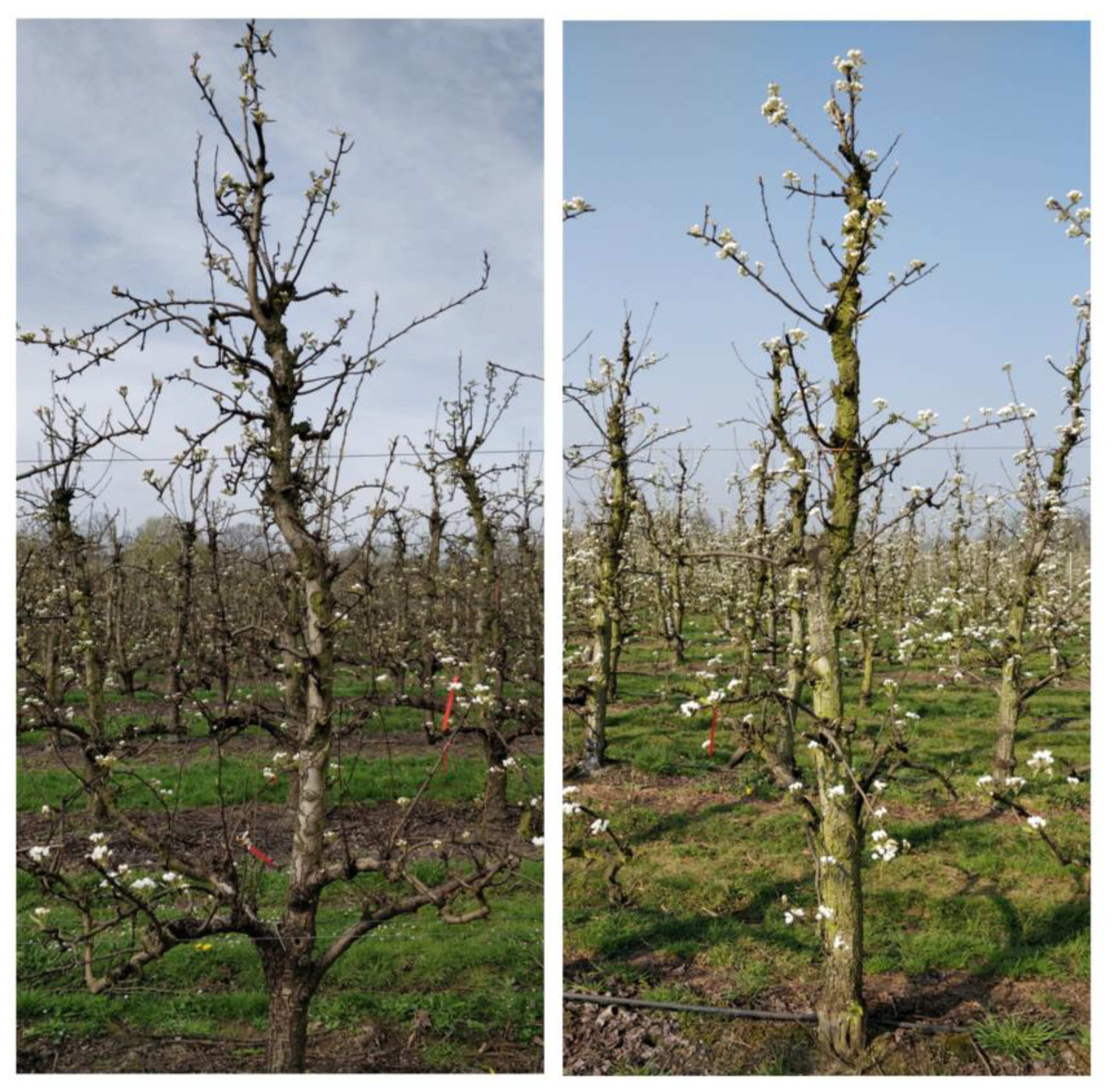
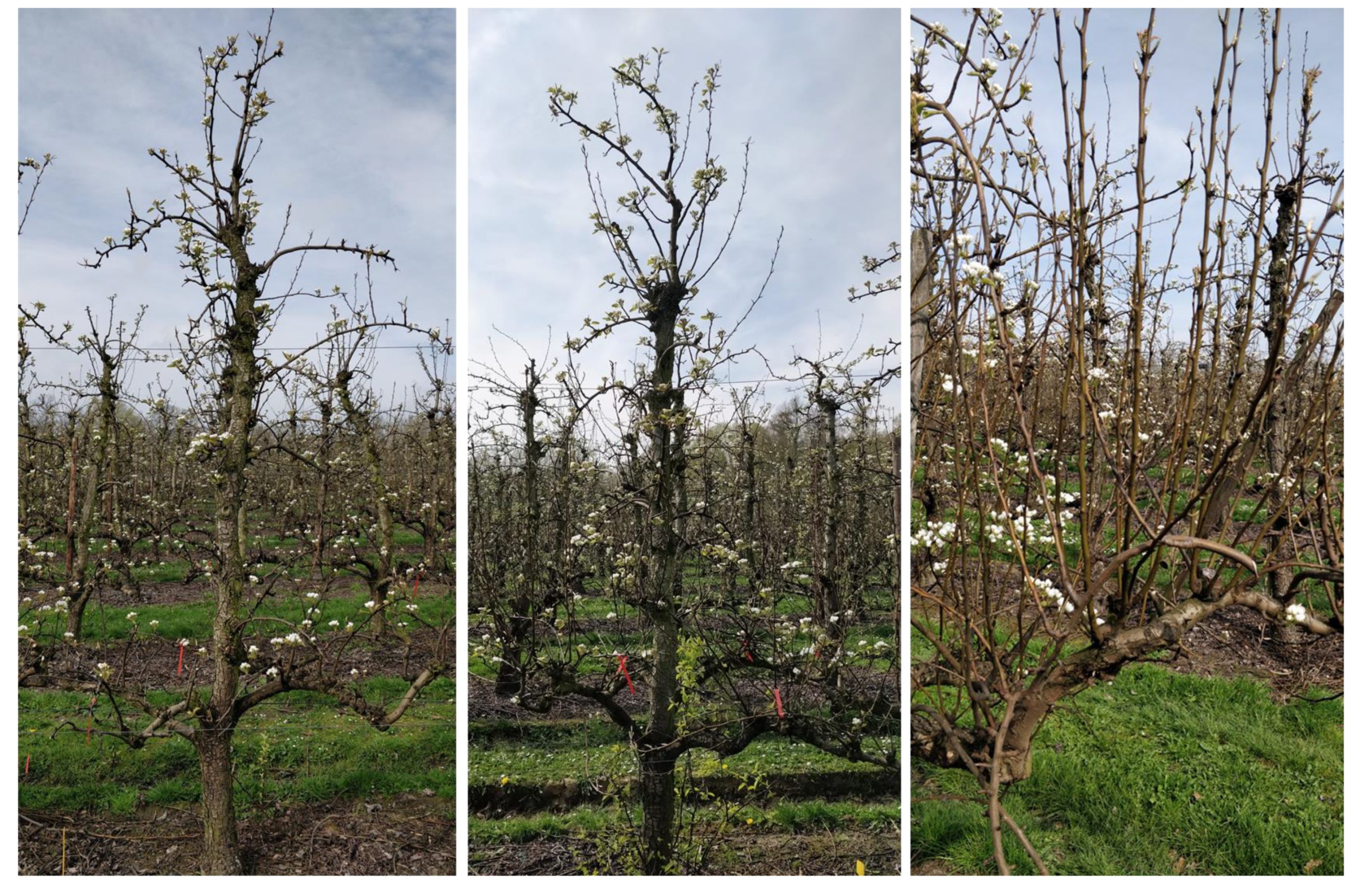
2.1. Study Area and Flower Cluster Reference Data

The orchards for this study were located in Wimmertingen, Belgium (50.892126 N, 5.341111 E) and Rummen (50.895398 N, 5.178401 E), Belgium. The trees in Wimmertingen were planted between 1992 and 1993 and grafted on Quince Adams rootstocks with a planting distance of 3.75 m × 1.5 m. Approximately every sixth row consisted of Doyenné du Commice trees, grafted on Quince C rootstocks, which acted as pollinators. The east–west oriented trees in Rummen were planted in the 1970s, except for the southernmost row which was planted in 2004. From the north–south oriented trees in Rummen, row 1 (starting at the east side) to row 34 and 40 to 50 were 25 years old, while row 35 to 39 were 15 years old. The planting distances were very variable in Rummen with a mean row distance of 3.5 m and a tree distance which varied between 1.5 and 2 m. The east–west oriented trees had on average a larger tree distance than the north–south oriented trees. The orchard in Rummen was irrigated, while the orchard in Wimmertingen was rainfed. The trees were trained in “Free spindle”. In this planting system, the trees have one central leader, and two lateral branches in the direction of the row, grown under an angle of 45°. Per orchard, a total of 24 plots of three trees each were monitored (Figure S1 in supplementary data).

Field-based flower cluster data was collected on the 18th of March 2019 by an experienced operator. The flower buds or clusters were counted at the phenological stage described by the Biologische Bundesantalt, Bundessortenamt, and Chemische Industrie (BBCH)- scale = 55 [26], when the flower buds were visible but not yet open. From the lower to the top branches the flower buds were counted. On average, an experienced counter obtains an error of 5% to 10%, with generally an underestimation of the real number of flower clusters due to hidden flower buds. In addition, image-based flower cluster data was also counted manually on the top-view RGB orthomosaic with the use of ImageJ [27]. This image-based flower cluster data is used to study the influence of the top-view perspective on flower visibility and hence the magnitude of the flower occlusion problem.

2.2. RGB Drone Data Acquisition

2.2.1. RGB Drone Data for Flower Cluster Estimation

The drone data for this research were captured over two commercial Conference pear orchards in Rummen and Wimmertingen (Belgium) at full bloom (BBCH 65) on the 10th of April 2019. The flights were executed with a commercially available Trimble UX5HP fixed wing drone, equipped with a Sony ILCE-7R, a 36 MP full-frame (4.88 µm pixel pitch) mirrorless interchangeable lens camera for RGB image acquisition. The Voigtländer 35 mm Color Skopar Pancake lens was used, which provided 54.3° cross-track field of view (FOV), resulting in 1 cm ground sample distance (GSD) from a flight height of 75 m above ground level (AGL) in Wimmertingen or 1.2 cm from the legal flight ceiling of 90 m AGL in Rummen. The system was designed specifically for surveying, with a metrically stabilized camera system (consisting of a screw mount and mechanical focus and aperture locking screws) to improve photogrammetric accuracy. The UX5HP is also equipped with a dual frequency patch antenna connected to a global navigation satellite systems (GNSS) receiver. Hence, image positions can be inferred with 2–5 cm accuracy through post-processing kinematic (PPK) calculation of the flight trajectory. Rough inertial measurement unit (IMU) data were also recorded for every image separate from the PPK analysis. The camera was operated with a fixed shutter speed and variable but capped ISO value in order to prevent forward motion blur while maximizing light capture, evening out brightness fluctuations and preventing excessive noise. The flight plan ensured 85% sideward and around 60%–70% forward image overlap. Flight planning, monitoring, vignetting correction and flight data export was done in the Trimble Aerial Imaging software, and PPK correction of image positions was done in Trimble Business Center 5×. Two or three artificial ground control point (GCP) markers were installed per field in Wimmertingen and Rummen, respectively, to ensure and validate georeferencing accuracy. The position of the ground control points was measured in the field using real-time kinematics (RTK) GNSS, taking corrections from a virtual reference station (VRS) in the Flemish positioning service (FLEPOS) network, with an average horizontal accuracy of around 2 cm and an average vertical accuracy of around 3 cm.

2.2.2. RGB Drone Data for Training the Pixel-Based Classifier

Four additional drone datasets were collected and used to retrieve regions of interest (ROIs) for training the pixel-based classifier (Section 2.3.2): in 2019, two preceding flights were done over the same orchards on the 5th of April 2019 (BBCH 60–61) with the same flight characteristics as in Section 2.2.1. In 2018, initial drone flights were conducted over the two orchards in the period of full bloom (BBCH 65) on the 18th of April. For the 2018 flights, a DJI Phantom 4 Pro was used. It has a 1” 20 MP (2.4 µm pixel pitch) RGB camera and an 8.8 mm autofocusing variable aperture lens, resulting in a 73.5° cross-track FOV and 1 cm GSD from a flight height of 38 m AGL over both study areas. An overlap of 85% in all directions was maintained to preserve photogrammetric accuracy. The DJI Phantom 4 Pro has a commercial grade GPS for image geotagging with an accuracy of several meters, and does not store IMU measurements in the image metadata. Therefore, at least seven GCP markers were installed per field in 2018, of which five were used as input in camera calibration and georeferencing, and at least two as independent check points. Several contiguous flights were needed to cover the entire extent of each orchard, which were processed together into one set of photogrammetric deliverables per field.

2.3. Data Processing

In this study flower cluster estimation from a more conventional flower cluster estimation approach based on top-view orthomosaics (i.e., a 2D approach) (Figure 1) was compared with the potential of drone imagery for flower cluster estimation from the colored dense point clouds (i.e., a 3D approach) (Figure 2). As the main focus of this study is on the imagery of the 10th of April 2019 and the preceding drone datasets were only used for training the pixel-based classifier, the difference between the 2018 and 2019 image processing workflows is explained in the Supplementary Material. First, the drone data of the 10th of April 2019 was processed to generate the colored dense point cloud, the orthomosaic, the digital surface (DSM) and the terrain model (DTM) (Section 2.3.1). Next the 2D (Figure 1) and 3D approaches (Figure 2) for flower cluster quantification were evaluated with a pixel-based (Section 2.3.2) and an object-based method (Section 2.3.3). Furthermore, the four methods were always tested on two sampling levels, namely at individual tree level and at plot (i.e., three consecutive trees) or multi-tree level.

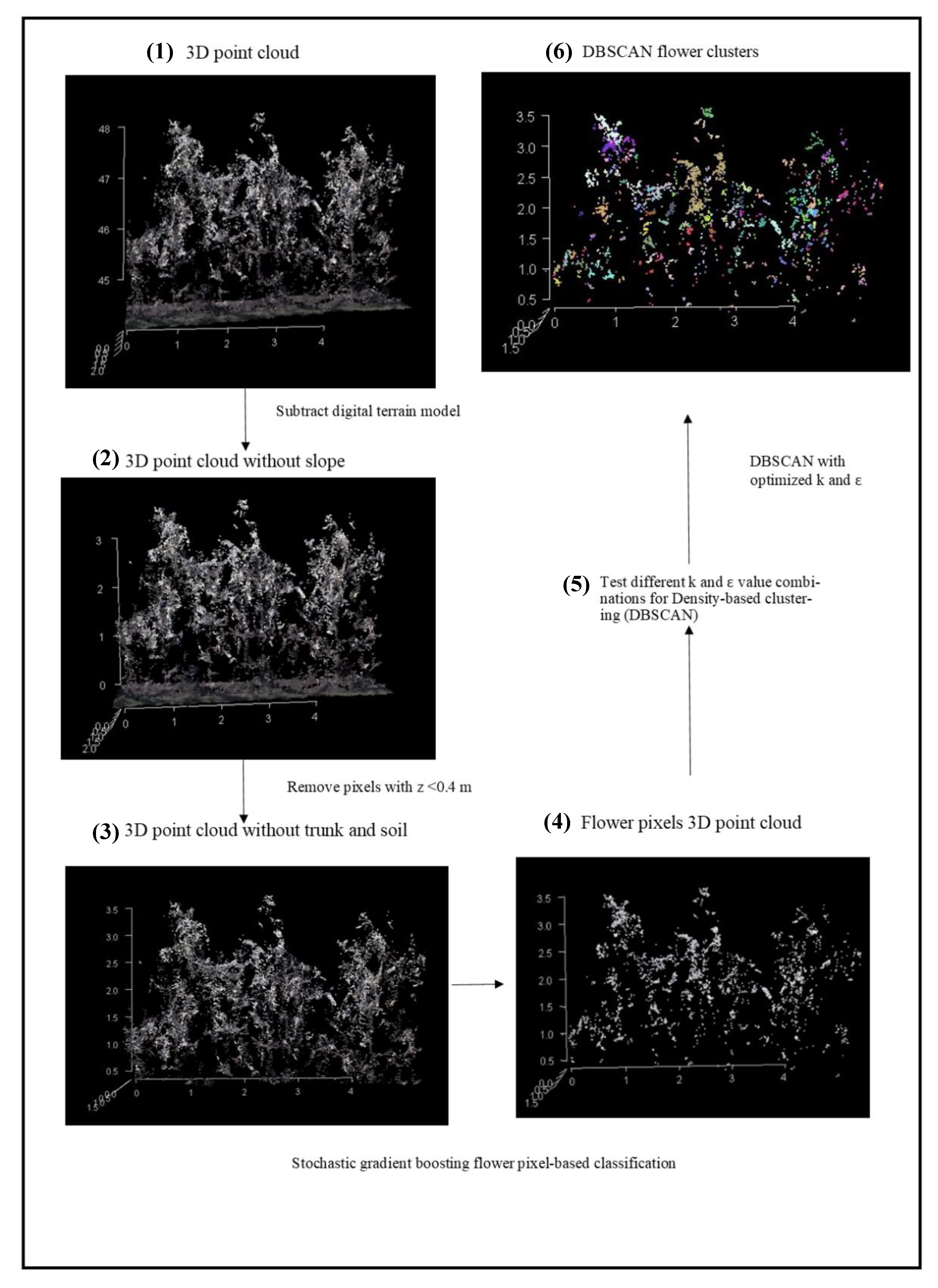
2.3.1. Colored Dense Point Cloud, Digital Elevation Model and Orthomosaic Generation

The collected drone images were processed through structure from motion (SfM) photogrammetry in the commercial software Agisoft Metashape Pro 1.5×. The SfM workflow consisted of seven steps: (1) tie-point extraction and matching (alignment), (2) geometric camera self-calibration and refinement of the georeferencing (optimization), (3) dense point cloud generation, (4) dense point cloud classification, (5) digital surface model (DSM) generation, (6) digital terrain model (DTM) generation, and (7) orthomosaic generation based on the DTM.

The alignment was done at image pyramid level 2. The geometric camera self-calibration optimized for focal length (f), principal point (cx, cy), skew and aspect ratio (b1, b2), three radial distortion coefficients (k1–k3) and two tangential coefficients (p1, p2). Camera self-calibration was done entirely relying on the precise image position measurements, while the absolute georeferencing (eliminating any potential global shifts) was done using one GCP marker, using the remaining point(s) as independent check point(s). Each GCP was indicated in at least nine overlapping images, with care taken to maximize the observation angles of the GCP markers. Check points were used for independent accuracy assessment, to ensure the output products were characterized by an absolute accuracy in the range of the image GNSS measurements (2–5 cm).

Dense point cloud generation was done at image pyramid level 1 with depth filtering disabled. For each point in the dense point cloud, the corresponding RGB color was computed. Next, the dense point cloud was classified into ground, above-ground and noise classes using a topographic filter with threshold values relating to maximum angle, maximum distance and search grid cell size. Using the classified dense point cloud the DSM was generated based on the ground and above-ground point classes and the DTM was generated based on the ground points only. Both were generated at a GSD twice that of the original image (corresponding to the level 1 dense point cloud extraction). Finally, the orthomosaics were generated based on the DTM. Examples of the resulting orthomosaic and colored dense point cloud are shown in Figure 1 and Figure 2.

Next, the individual trees had to be extracted from the orthomosaics and colored dense point clouds. As reported in earlier studies, it can be very difficult in pome orchards to see where one fruit tree ends and the other tree begins since the branches are strongly intertwined in trees with a spindle structure and a small planting distance [16]. Nevertheless, tree delineation can have a significant effect on the performance of the 2D and 3D flower cluster models. In order to partly decouple the effect of tree delineation on the performance of the flower cluster models, these models will be evaluated on ‘per tree’ and ‘per plot’ (i.e., three consecutive trees) level. On plot level there are only two boundaries, while on per tree level there are six boundaries to be drawn were a delineation error can occur. Based on the orthomosaics, rectangular bounding boxes were created to delineate each tree or plot (Figure 1, step 2). The bounding boxes were manually drawn and stored as polygon shapes in QGIS 3.4. Next, the plot and tree orthomosaics were exported using the extract function from the package “raster” in R [28]. The plot and tree dense point clouds were exported with the readLAS function of the package “lidR” in R using the coordinates of the bounding boxes to extract each plot or tree [29].

For the 3D approach, the background of the colored dense point clouds was removed (Figure 2, step 2 and Figure 3) to reduce the processing time and to further reduce the flower classification error since some soil elements and pruned branches on the ground appear white and might be classified as flower pixels. First the slope of the terrain had to be removed. This was done by extracting the digital terrain model (DTM) of each tree or plot with the crop function of the “raster” package in R [28]. Secondly, the aggregate function from the “stats” package was used to reduce the spatial resolution with a factor of 3 in order to enhance the processing time of the next steps [30]. Thirdly, the focal function of the “raster” package was used to smooth the surface of the DTM by applying a median moving window of 31 × 31 pixels [28]. This step was needed since the DTM generation in the first processing section still contained some artifacts from the tree (e.g., the DTM still showed the tree rows as minima). The smoothed DTM was then subtracted from the z-axis of the point cloud of each tree or plot (Figure 2, step 2). This resulted in a point cloud with all tree bases at a height of 0 m instead of following the slope of the field. Next, the tree trunk, soil points and the ghost points below the soil were removed by removing the points under 40 cm on the z-axis (Figure 2, step 3).

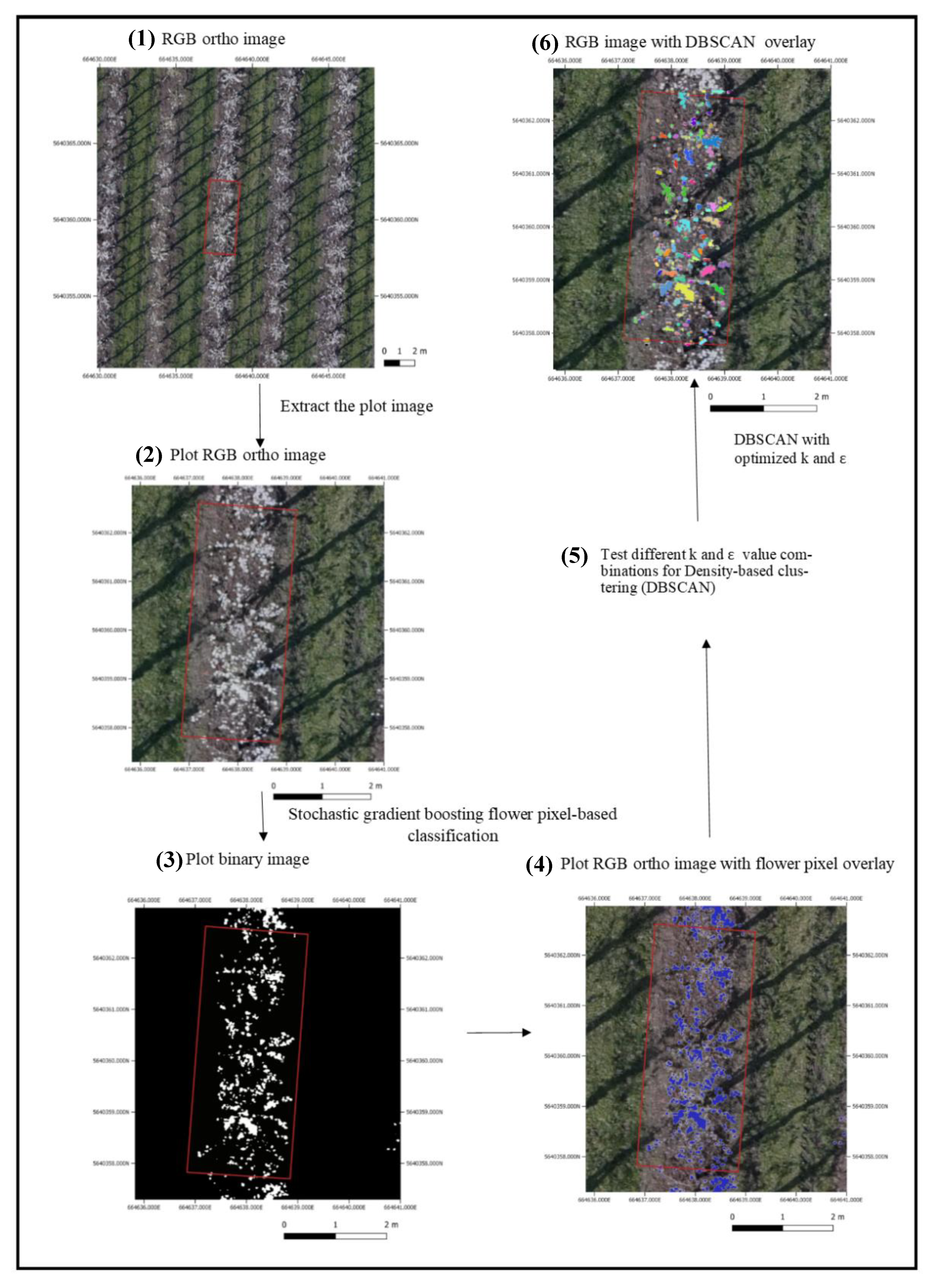
2.3.2. Pixel-Based Flower Classification

A pixel-based classification method, namely Stochastic Gradient Boosting (SGB) [31] was used to identify the flower pixels. SGB is an advanced machine-learning tree ensemble method similar to bagging and boosting techniques and was the preferred algorithm since it was faster and had the same accuracy as random forest for our dataset (results for random forest not shown). The SGB algorithm builds classification trees sequentially whereby at each iteration a tree is grown from a random sub-sample of the data without replacement. While the model utilizes a stepwise fitting approach to reduce the effects of bias, a residual error is computed on the data that are not used in the fitting procedure. SGB then retains the number of trees that produces the lowest residual error for classification. In addition, stochasticity is introduced to improve model performance and reduce chances of overfitting [31]. The main strengths of the SGB algorithm include: (i) resistance to outliers, (ii) use of predictor variables without transformation, (iii) the capability of fitting complex non-linear relationships, and (iv) the automatic handling of interaction effects among predictors [32]. A total of 100 regions of interests (ROIs) were selected in each of the six RGB images (two fields × three flight times) (Section 2.2), amounting to over 275,900 pixels, as training and calibration data. The algorithm was repeated 1000 times with a 5-fold cross validation. The “caret” and “gbm” R packages were used to run this analysis [33,34]. Next, the trained SGB algorithm was performed on the orthomosaics and the dense point cloud, resulting in a binary classified image and point cloud. The number of flower pixels per tree or plot were determined by taking the sum of the pixel values (i.e., flower pixel value = 1, background pixel value = 0) present in the respective binary image or binary point cloud. These results are the flower cluster estimations for the 2D pixel-based method (i.e., 2D flower pixels) and the 3D pixel-based method (i.e., 3D flower pixels).

2.3.3. Flower Pixel Clustering

In order to cluster the flower pixels into objects, density based spatial clustering (DBSCAN) [35,36] was performed on the SGB classified (i.e., binary) orthomosaics (Figure 1) and the binary point cloud (Figure 2). DBSCAN uses a simple minimum density level estimation, based on a threshold for the number of neighboring points, k, within the radius ε (an arbitrary distance measure). Objects with more than k neighbors within this radius (including the query point) are considered to be a core point. The intuition of DBSCAN is to find those areas which satisfy this minimum density, and which are separated by areas of lower density. For efficiency reasons, DBSCAN does not perform density estimation in-between points. Instead, all neighbors within the ε radius of a core point are considered to be part of the same cluster as the core point. If any of these neighbors is again a core point, their neighborhoods are transitively included. Non-core points in this set are called border points, and all points within the same set are density connected. Points which are not density reachable from any core point are considered noise and do not belong to any cluster [37]. The parameters k and radius ε had to be determined for the 2D and 3D approach. K is the minimal number of flower pixels needed to form one flower cluster. To obtain a range of k, the flower pixels determined in Section 2.3.2 were divided by the reference number of flower clusters for each tree counted on the orthomosaic for the 2D approach. For the 3D approach, the flower pixels were divided by the flower clusters counted on the ground. This step was performed to get an idea of the minimum number of flower pixels which form one flower cluster and thus one object.

Next, the minimum value of the obtained range was taken as a maximum value for k (i.e., k_max). A range of k between one and k_max was evaluated as possible values for k. Another option to get an estimation of k_max is to go for a physical-based approach and assume a flower cluster has seven to nine flowers and each flower has a diameter of 1–2 cm at full bloom. As the GSD is 1 cm, k should be at least seven. However, this method does not take into account the variability in phenology which can be present between trees and thus an optimal k could be smaller than seven. In addition, the density of the 3D point cloud decreases from the top of the canopy towards the soil, which also entails that an optimal k could be smaller than 7. In addition, for the 2D approach, due to flower overlap, the k might also be lower than 7. The other parameter ε is dependent on k and can be determined by computing a k-distance plot of the data. The inflection point of this curve is generally a good estimator of ε [38]. Points further than a distance ε from the groups of points are considered noise. Therefore, a range of ε values in the “knee” of the k-distance curves were tested to find the optimal value for ε, with a step size of 0.05.

2.4. Magnitude of the Flower Occlusion Problem

As mentioned in Section 2.1, to study the influence of the top-view perspective on the flower visibility, the number of flower clusters was also counted manually on the top-view orthomosaics with the use of ImageJ, both on plot and on tree level. The image-based flower clusters that were manually counted from the orthomosaic (i.e., image-based flower clusters FC_p*) were then compared with the field-based flower cluster number counted on the tree in the orchard (i.e., field-based flower clusters, FC_p) by calculating the coefficient of determination, R² (Equation (1)) and the relative root mean squared error, RRMSE (Equation (2)) between them for each orchard on both plot and tree level (Section 2.3.1). In Equation (1) and (2) $\overline{\mathrm{FC}}$ is the average field-based flower cluster number observed in the field; for both orchards, k is equal to 72 on tree level and 24 on plot level.

$${\mathrm{R}}^2=\frac{{{\displaystyle \sum }}_{p=1}^k{\left({\mathrm{FC}}_{\mathrm{p}}^{*}-\overline{\mathrm{FC}}\right)}^2}{{{\displaystyle \sum }}_{p=1}^k{\left({\mathrm{FC}}_{\mathrm{p}}-\overline{\mathrm{FC}}\right)}^2}$$

(1)

$$\mathrm{RRMSE}=\frac{\sqrt{{{\displaystyle \sum }}_{\mathrm{p}=1}^{\mathrm{k}}\frac{{\left({\mathrm{FC}}_{\mathrm{p}}^{*}-\overline{\mathrm{FC}}\right)}^2}{\mathrm{k}}}}{\overline{\mathrm{FC}}}$$

(2)

As the tree volume increases, the hypothesis is that flower occlusion might be larger. In order to visualize the effect of tree volume on the flower cluster estimation accuracies the tree volume of each tree or plot was also calculated. A proxy for the tree volume was calculated based on the canopy height model (CHM). For the CHM, the DTM was subtracted from the DSM. The tree or plot was extracted from the CHM and as a last step the pixel values of the CHM of each tree or plot were summed to get a proxy for the tree volume in cm³. As large canopies can still have an open architecture, the percentage and amount of overlapping flower clusters was also calculated. These parameters were calculated by projecting the colored dense point cloud of the flower pixels in the xy-space followed by taking the sum of the flower pixels with the same x and y coordinates.

2.5. Accuracy Assessment

2.5.1. Pixel-Based Classification

The accuracy of the pixel-based classifications (2D and 3D) were assessed by the mean overall accuracy (OA) and the mean Kappa coefficient ($\widehat{K})$ over all the data splits (i.e., 5-fold cross validation with 1000 repeats). The OAwas calculated by dividing the number of correct classifications by the total number of samples (i.e., pixels) taken [39]. The Kappa coefficient [40] is a measure of overall agreement of a matrix (Equation (3)). In contrast to the overall accuracy, the ratio of the sum of diagonal values to total number of cell counts in the confusion matrix, the Kappa coefficient takes also non-diagonal elements into account. The Kappa coefficient measures the proportion of agreement after chance agreements have been removed from considerations. Kappa increases to one as chance agreement decreases. A Kappa of zero occurs when the agreement between classified data and verification data equals chance agreement [41].

$$\widehat{K}=\frac{N{{\displaystyle \sum }}_{i=1}^r{X}_{ii}-{{\displaystyle \sum }}_{i=1}^r{X}_{i+}{X}_{+i}}{N^2-{{\displaystyle \sum }}_{i=1}^r{X}_{i+}{X}_{+i}}$$

(3)

In Equation (3), r = number of rows and columns in the error matrix, N = total number of observations, Xii = observation in row i and column I, Xi+ = marginal total of row i and X+I = marginal total of column i.

2.5.2. Optimization of DBSCAN Parameters

The optimal k and ε were chosen by performing a 5-fold cross validation repeated 100 times between the flower cluster number estimated by the object-based method (with a specific k and ε) and the field-based (for the 3D approach) and image-based (for the 2D approach) flower cluster number. The optimization step was performed in the “caret” R package with the linear regression model (i.e., lm) [33]. The optimal k and ε values for the DBSCAN algorithm for clustering were determined by the calculation of the mean and standard deviation of R² (Equation (1)) and of the RRMSE between the estimated number of flower clusters with the 2D and 3D object-based methods (FC_p^*) (Equation (2)) and the field-based flower clusters (FC_p) for the 3D approach and the image-based flower clusters (FC_p) for the 2D approach. The optimal k and ε on tree and plot level are given in Section 3.3.

2.5.3. Flower Cluster Estimation Methods

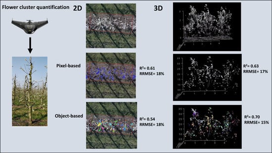
To assess the accuracy of the pixel-based and object-based methods for the estimation of the field-based flower clusters, the flower pixels and clusters respectively retrieved from both the classified orthomosaic (2D approach) and the classified colored point cloud (3D approach) were also compared with the field-based flower cluster number by calculating the R² (Equation (1)) and RRMSE (Equation (2)). For the 3D approach, the estimated number of flower clusters was based on the optimal k and ε of Section 2.4. Here, FCp is the field-based flower cluster number, FCp* is the estimated number of flower clusters for the pixel-based or object-based method, and k represents the number of measurements. For both orchards, k is equal to 72 on tree level and 24 on plot level.

3. Results

In this section there is first an evaluation of the magnitude of the flower occlusion from the top-view perspective (Section 3.1). Secondly, the performance of the pixel-based classification algorithm for flower pixel segmentation is assessed (Section 3.2). Next, the parameters k and ε are optimized for clustering the flower pixels into flower object with the use of DBSCAN (Section 3.3). Finally, the four methods to estimate the number of flower clusters are compared (Section 3.4), namely, the pixel-based 2D method (i.e., 2D flower pixels) on the orthomosaics (Figure 1) and the pixel-based 3D approach (i.e., 3D flower pixels) using the colored dense point cloud (Figure 2). The last two methods are named the 2D and 3D object-based methods.

3.1. Magnitude of the Flower Occlusion Problem

In order to evaluate if the image-based flower cluster number is truly representative for the field-based flower cluster number, both numbers were compared (Figure 3). In previous drone studies only the top-view perspective was used and assumed to be representative for the entire tree [10,16,18,23]. Therefore, the performance of the flower cluster estimation method could not be decoupled from the effect of viewing perspective in these studies. This analysis was done to evaluate if it is necessary to include more viewing perspectives to reduce flower occlusion. For the field-based flower clusters on each tree level both orchards had a similar mean (i.e., 150) and range with a minimum number of 50 flower clusters and a maximum of 300 flower clusters per tree. For the image-based flower clusters, the orchard in Rummen had a smaller range (59–164) and mean (109) than the orchard in Wimmertingen (range = 41–179 and mean = 116). The top-view of the fruit trees in Rummen (Figure 3a,b) gave a better representation of the flower clusters present on the entire tree than for Wimmertingen (Figure 3c,d). Image-based flower clusters from top-view of the trees showed as much as 76% of the flower cluster variability present in Rummen (Figure 3b), while only 50% of the flower cluster variability was visible for Wimmertingen (Figure 3d). When looking at the trees at individual tree level, only 42%–43% of flower cluster variability was visible. The accuracy difference of 26% between both orchards can be largely explained by differences in tree volume/density as the trees in Wimmertingen (Figure 3c,d) have a much larger canopy than the trees in Rummen (Figure 3a,b). Furthermore, the percentage of overlapping flower pixels (i.e., pixels with the same x and y coordinate) was 33% for both orchards. However, in absolute numbers, the amount of overlapping flower pixels was higher for Wimmertingen (average 1603 overlapping pixels) than for Rummen (average of 1188 overlapping pixels). In Wimmertingen, the number of overlapping flower pixels of the unpruned trees (average overlapping pixels = 1707) was also higher than for the pruned trees (average overlapping pixels = 1561). Due to this large discrepancy in top-view accuracy between the orchards, both are treated separately in the next sections.

3.2. Accuracy of the Pixel-Based Classification

The flower pixel classification with SGB resulted in a mean overall accuracy of 0.97 and a Kappa coefficient of 0.84. This was based on the 5-fold cross validation with 1000 repeats of the 275,900 pixels used for training and calibration. Next, the trained SGB was applied on the orthomosaic and colored dense point cloud of the 10th of April 2019 on plot and tree level to calculate the number of flower pixels for the 2D and 3D pixel-based methods for estimating the field-based flower clusters and the 2D and 3D flower pixels are also the input for the clustering in the next section (Figure 1 and Figure 2).

3.3. Optimalisation of DBSCAN Parameters

Finally, DBSCAN with varying k and ε parameters was performed on the 2D and 3D flower pixels on tree and plot-level. The results of this step are given in

Table 1. Optimal DBSCAN parameters k and ε with accuracy metrics R², RMSE and RRMSE with standard deviation between brackets for Rummen.

	K	ε	R2	RMSE	RRMSE
2D Object-based tree	1	0.005	0.72 (0.10)	15 (2)	14% (2%)
2D Object-based plot	2	0.012	0.81 (0.14)	34 (8)	10% (2%)
3D Object-based tree	12	0.11	0.44 (0.15)	33 (8)	23% (6%)
3D Object-based plot	16	0.135	0.71 (0.2)	60 (16)	14% (4 %)

for Rummen and

Table 2. Optimal DBSCAN parameters k and ε with accuracy metrics R², RMSE and RRMSE with standard deviation between brackets for Wimmertingen.

	K	ε	R2	RMSE	RRMSE
2D Object-based tree	9	0.019	0.60 (0.16)	19 (4)	16% (3%)
2D Object-based plot	9	0.022	0.87 (0.10)	32 (9)	9% (3%)
3D Object-based tree	1	0.06	0.45 (0.17)	33 (6)	23% (4%)
3D Object-based plot	13	0.12	0.70 (0.21)	64 (18)	15%(4%)

for Wimmertingen. The k and ε values given are those resulting in the highest R² and smallest RRMSE in combination with the smallest standard deviation.

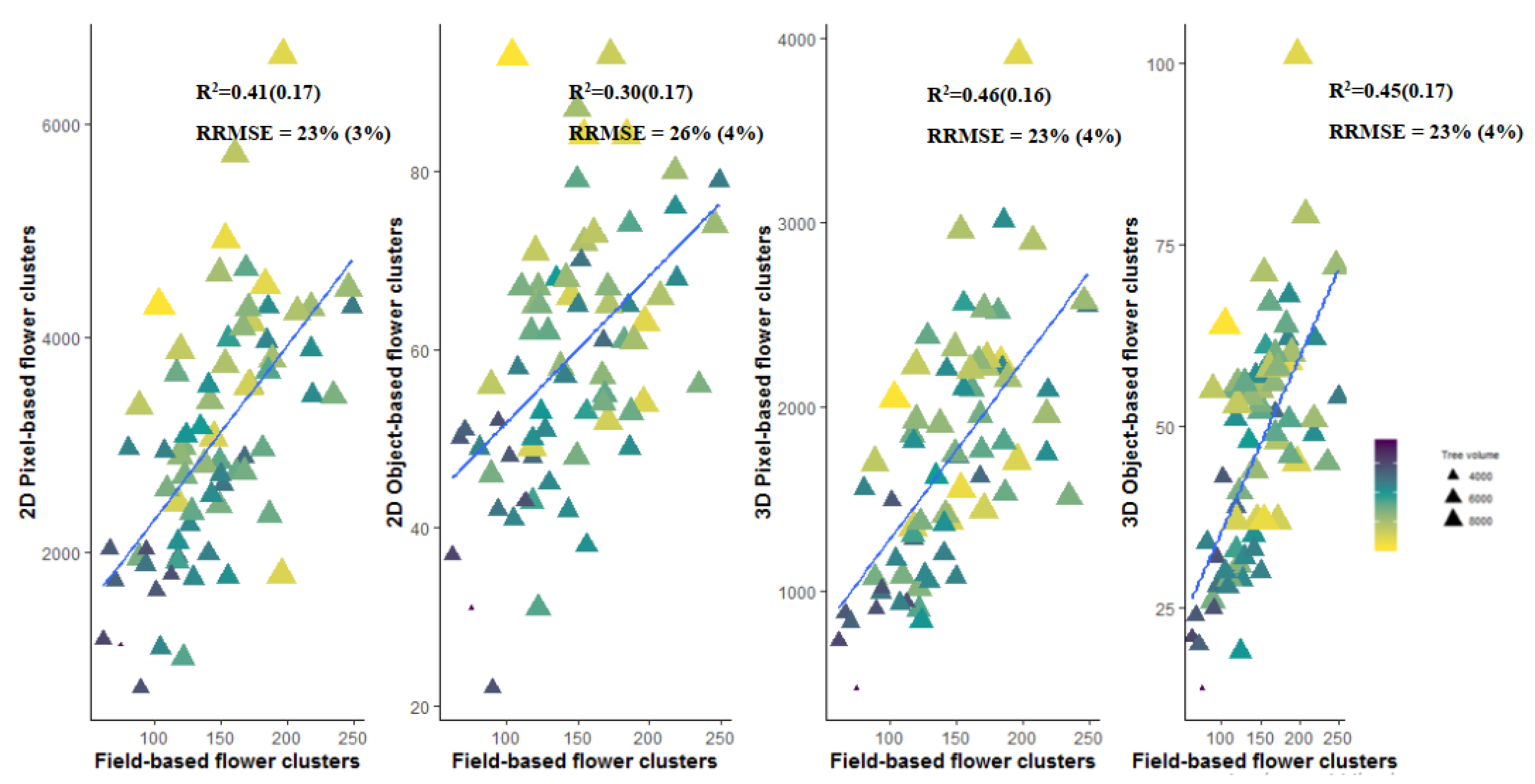
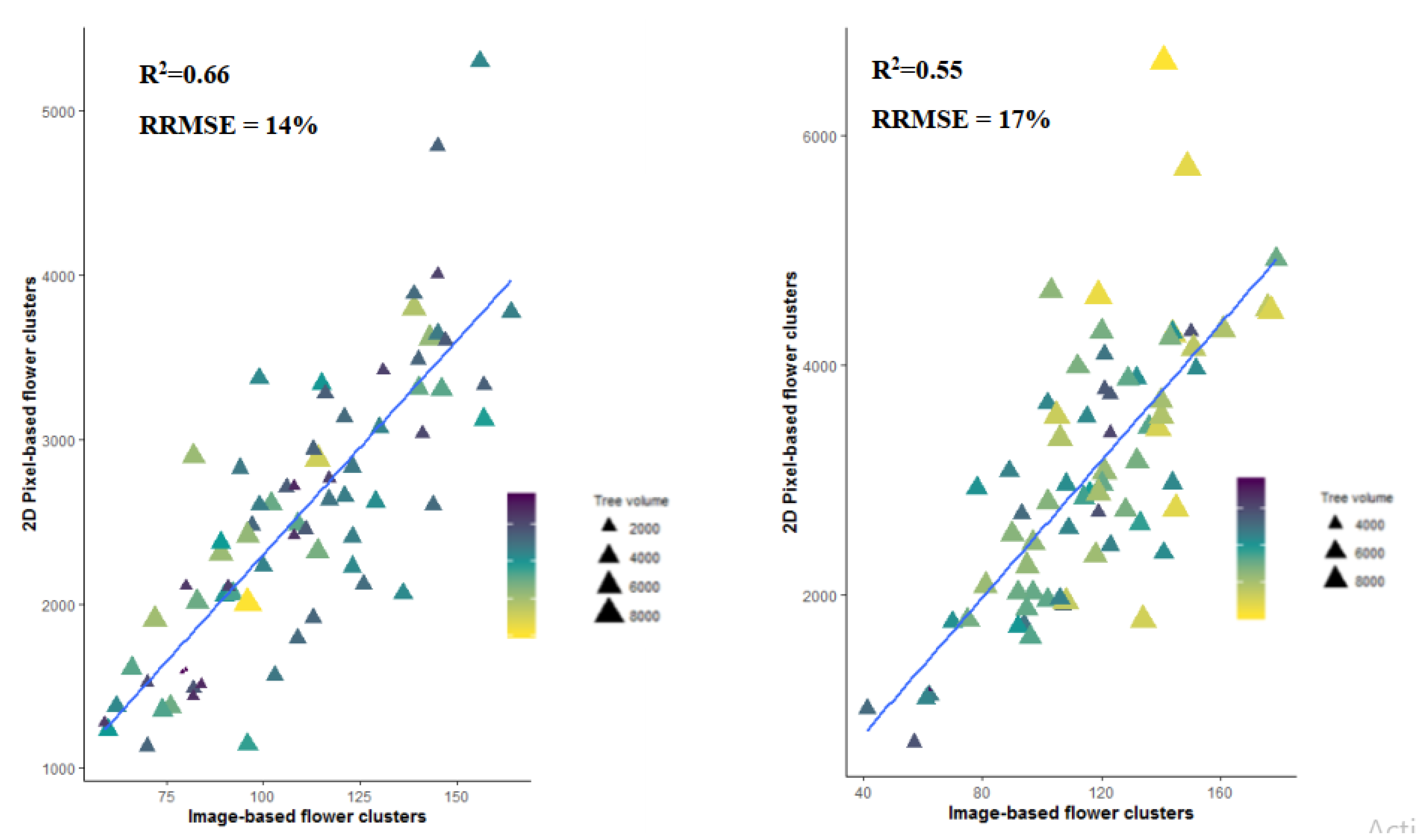
3.4. Flower Cluster Estimation Models

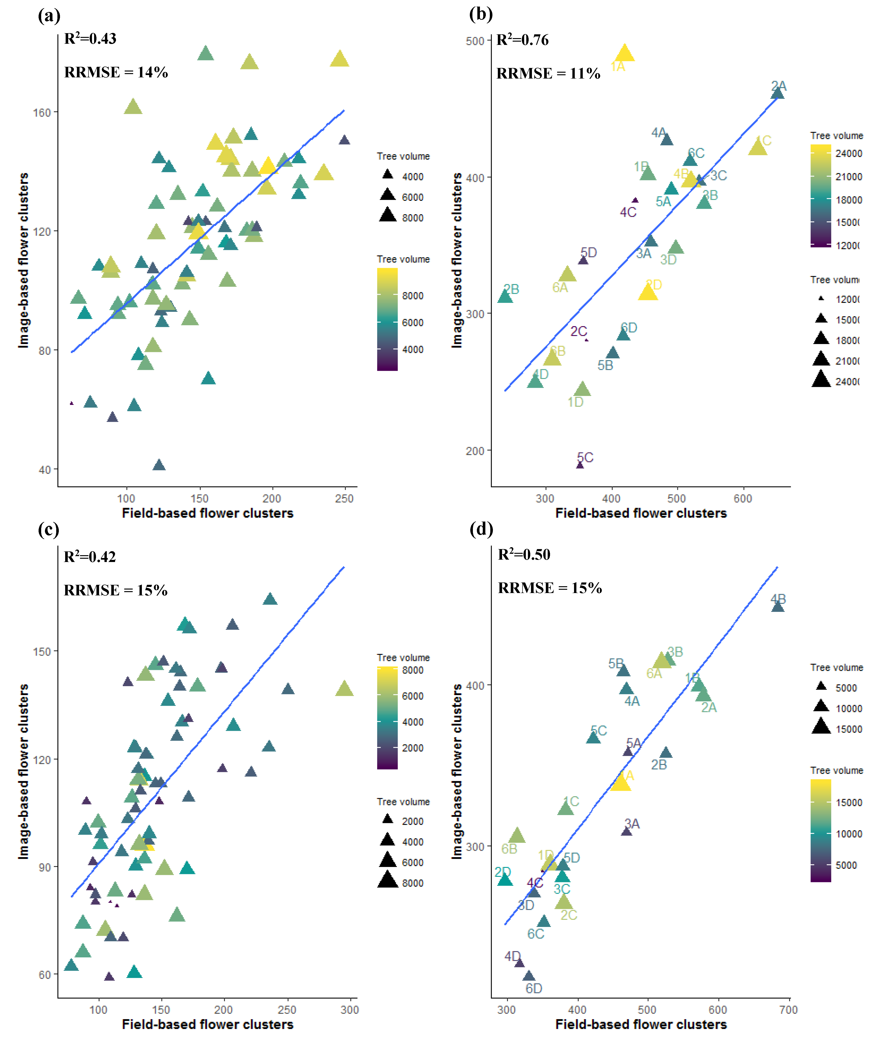
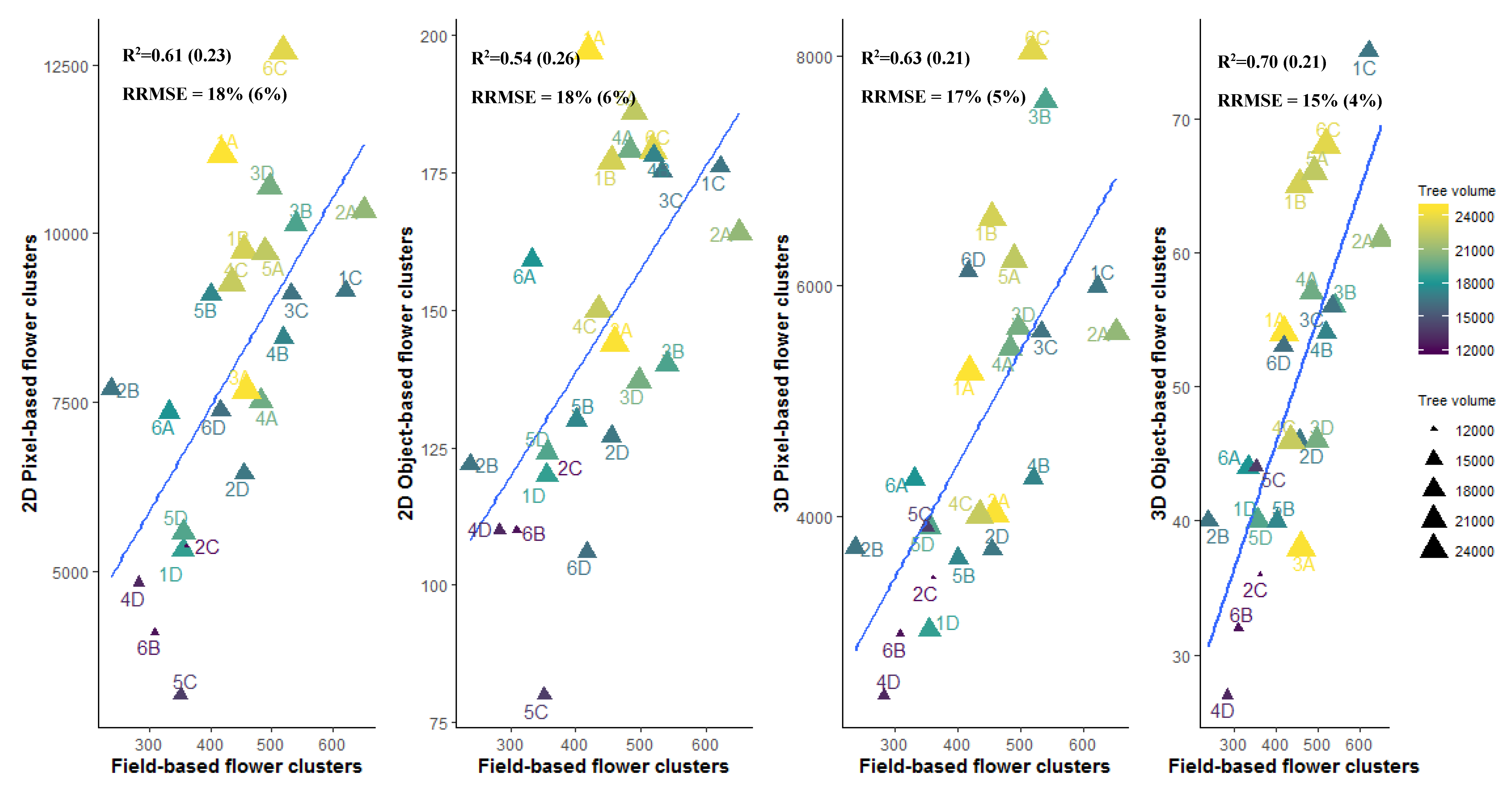
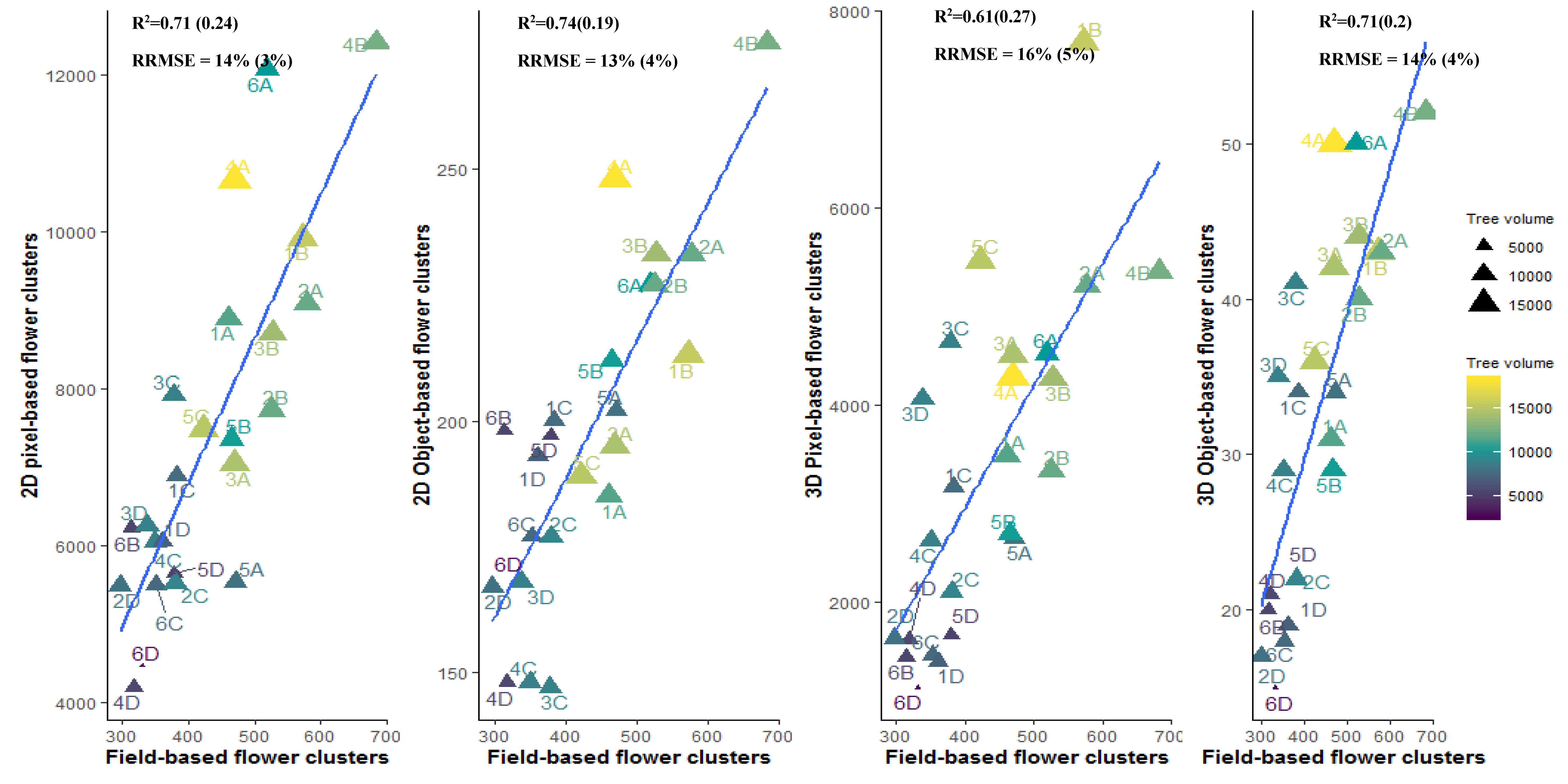
3.4.1. Individual Tree Level

On individual tree level all four methods performed similarly for both Rummen and Wimmertingen with a mean R² of 0.30–0.46 and an RRMSE of 23%–26% (Figure A1 and Figure A2). These results agree with the findings in Figure 3 which showed that image-based flower clusters of the tree show about 42%–43% of the variability of the field-based flower cluster numbers for both orchards. The RRMSE is however larger for the pixel and object-based methods (RRMSE: 22%–26%) (Figure A1 and Figure A2) than by image-based flower cluster counting (RRMSE: 14%–15%) (Figure 3). In addition, when comparing the results of the 2D pixel-based method with the image-based flower clusters we see that the automated method performs better for the Rummen orchard (R² = 0.66, RRMSE = 14%) than for the Wimmertingen orchard (R² = 0.55, RRMSE = 17%) (Figure A3).

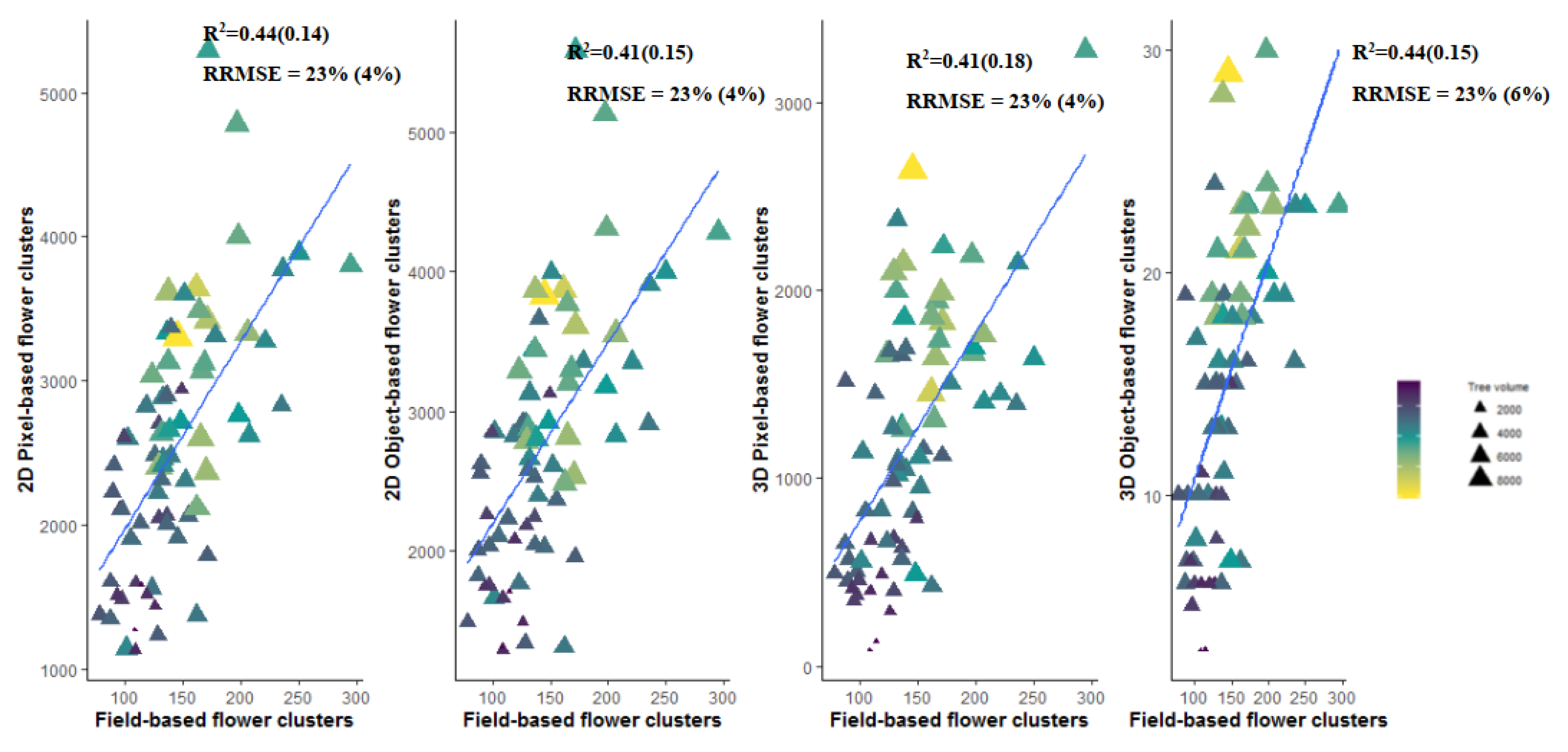
3.4.2. Plot or Multiple Tree Level

On plot level the 3D object-based method (3D object-based: R² = 0.7, RRMSE = 15%) performs significantly better than the 2D object-based method for Wimmertingen (2D DBSCAN: R² = 0.54, RRMSE = 18%), the difference in performance between the 2D pixel-based and 3D pixel-based methods is much smaller (Figure 4). For Rummen the difference between the performance of the 2D (2D pixel-based: R² = 0.71, RRMSE = 14%; 2D object-based R² = 0.74, RRMSE = 13%) and the 3D methods is smaller (3D pixel-based: R² = 0.61, RRMSE = 16%, 3D object-based: R² = 0.71, RRMSE = 14%) (Figure 5). This confirms the observation of Section 3.1 that for Rummen the top-view perspective is already a good representation of the entire tree with R² = 0.76, hence there is less room for improvement than for the Wimmertingen orchard with R² = 0.50 (Figure 3). For the Rummen orchard there are some outliers in the third graph, namely 3C, 3D and 5C (Figure 5). For these plots, the 3D pixel-based method overestimates the number of flower clusters. When the outliers are removed, the accuracy of the 3D pixel-based method increases to R² = 0.73 (0.15) and the RRMSE decreases to 14% (6%). Without the outliers the 3D object-based method (with k = 15 and ε = 0.11) gives a R² = 0.85 (0.13) and RRMSE = 10% (2%) for estimating the field-based flower clusters.

4. Discussion

4.1. Viewing Perspective

In Rummen the top-view perspective showed 76% of the variability in flower clusters compared to only 50% for Wimmertingen. This was probably caused by different pruning techniques in both orchards, which translated into tree volume, shape and density differences. In addition, part of the trees of the Wimmertingen orchard (plot: 1C, 1D, 2A, 2C, 2D, 3B and 3C) were not yet pruned at the time of the drone flight. Examples of pruned and unpruned trees are given in Figure A5. In Rummen the trees had a more open structure with shorter branches compared to Wimmertingen (Figure A4), leading to a smaller tree volume (Figure 3) and hence less overlap of flower clusters for the trees in Rummen. Therefore, the 2D methods using only the top-view perspective sufficed to get accurate estimations for trees with this open architecture as was confirmed by the results in Figure 5. For Rummen, the most accurate 3D method (R² = 0.71, RRMSE = 14%) had the same accuracy as the most accurate 2D method (R² = 0.74, RRMSE = 14%). As expected, for Wimmertingen the most accurate 3D approach did indeed perform significantly better (R² = 0.71, RRMSE = 15%) than the most accurate 2D method (R² = 0.61, RRMSE = 17%). Based on these results, it can be concluded that the 3D viewing perspective is preferred for trees with a larger/denser canopy and more flower overlap. This also entails that reported accuracies in previous studies of flower cluster number estimation methods are highly dependent on tree architecture and viewing perspective. Therefore, these studies are difficult to compare with each other. For example, Tubau et al. (2019) [16] achieved an accuracy of R² = 0.56 with a 2D pixel-based approach for estimating the field-based flower cluster numbers, while in this study accuracies between R² = 0.61 and R² = 0.71 were achieved with the 2D pixel-based approach (Figure 4 and Figure 5). As classification accuracies were not reported in their study it is impossible to know if this difference in flower number estimation accuracy is due to the performance of the pixel-based classification algorithm or due to a difference in tree architecture or even tree delineation.

The comparison of the flower cluster estimations from the 2D pixel-based methods (R² = 0.71, RRMSE = 14% (Rummen); R² = 0.61, RRMSE = 18% (Wimmertingen)) with the image-based flower clusters (R² = 0.76, RRMSE = 11% (Rummen); R²=0.5, RRMSE = 16% (Wimmertingen)) showed there was still room for improvement for flower cluster estimations from the top-view perspective. For the 3D pixel approach the results for Rummen (R² = 0.61, RRMSE = 16%) and Wimmertingen (R² = 0.63, RRMSE = 17%) were also not optimal yet. For Rummen, the 3D pixel-based method performed even worse than the 2D pixel-based method. The third graph of Figure 5 shows the three outliers (plots 3C, 3D and 5C) causing this lower accuracy. For these plots, the 3D pixel-based method overestimated the number of flower clusters. In this part of the orchard, the dense point cloud showed more noise, visible as points above and below the surface. Although the exact cause of the excessive noise is unknown, it is worth noting that an E–W oriented flight block intersected with a N–S oriented flight block in this area, resulting in an excessive overlap of differently oriented images with slightly different light characteristics. Regardless of the cause, the noise may have let neighboring pixels belonging to the same flower cluster in the original images being erroneously projected in divergent 3D positions within a certain tree or even neighboring trees, thus resulting in an overestimation of the number of flower clusters. Different levels of noise filtering can be applied in the dense point cloud extraction, but increasing the filtering to reduce the noise in this area led to removal of the true details in other areas of the point cloud. A potential method that preserves the information coming from oblique observation angles in the original imagery and the geometric accuracy coming from bundle adjustment and camera calibration (with or without GCPs next to PPK GNSS positioning) while avoiding the issue of noise that comes with dense point cloud extraction is detailed in Baeck et al. (2019) [42]. As such, it can be considered a hybrid approach between the 2D and 3D methods described in this study. However, this approach is yet to be tested on the identification of flower clusters.

4.2. Tree Delineation

For all methods, sampling at plot level (multiple tree level) led to significantly higher accuracies than with sampling at individual tree level (Table 1, Table 2 and Figure 4, Figure 5, Figure A1, Figure A2). Note that the RMSE mentioned in Table 1 and Table 2 on plot level are per three trees. In order to compare them with the RMSE on ‘tree level’ they should be divided by three. The higher accuracy on ‘plot level’ was expected (see Section 2.3.1) since there are six delineation borders for three individual trees while there are only two for the plot level approach. Each delineation border between the consecutive trees is prone to errors in delineation since the tree branches are highly overlapping. Expert counters in the field sometimes even need to follow the branches until the tree trunk to know to which tree they belong. In this study, the colored dense point clouds were, however, not dense enough (i.e., branches were not completely visible) to create an automated tree segmentation method based on this modus operandi. Furthermore, there is also the question if individual tree delineation for flower cluster estimation per tree is really necessary for practical use. Growers will use the flower cluster estimations to steer pruning and flower thinning, and to get early yield estimations. For example, for yield estimations, knowing the flower clusters per tree instead of per meter will probably lead to higher estimation accuracies since the flower clusters determine the amount of sinks and the carbohydrate balance of its tree, and hence determine the physiological fruit fall of one particular tree [43]. If pear trees show a gradual change in flower clusters according to their position to the neighboring trees individual tree delineation is not necessary. However, when there is an abrupt change in flower cluster numbers between two neighboring trees, individual tree delineation would be preferred.

Abrupt changes in flower cluster numbers can, for instance, be caused by a local infection (e.g., fire blight) [44] or the presence of a pollinator alternated in the same row [45]. These pollinators have to bloom at the same time as the commercial cultivar of interest but the flower phenology might start earlier or later in these cultivars. For example for ‘Conference’ and its pollinator ‘Doyenné du Comice’ the duration of flowering is about 10 days, with an overlap of 7.5 ± 1.5 days, and flowering starts slightly later for Doyenné du Comice [45]. If a drone flight would be conducted when the Conference trees are already flowering while the pollinator is not, this will lead to an underestimation of the flower cluster numbers for the pollinator. Although the commercial pear cultivar is of main interest for the grower, information about the pollinator and flowering phenology could give an indication of the effectiveness of the pollinator. For mechanization systems of pruning and flower (bud) thinning the issue of overlapping branches was also mentioned [10]. Follow-up studies are needed to investigate and quantify the need for per meter or per tree flower cluster assessment for specific management tasks.

4.3. Pixel-Based Versus Object-Based Classification

In order to evaluate if an object-based method could lead to higher accuracies, the flower pixels from the 2D and 3D pixel methods were grouped in flower cluster objects with the use of DBSCAN. It should be noted that the object-based method is not completely independent of the pixel-based method since the pixel-classification error, although minimal (OA = 0.97), will be propagated in the clustering method. As mentioned in the introduction, in previous studies of other pixel-based classifiers both color-based thresholding techniques and (un)supervised classifiers were used. As the supervised classifiers are more robust to illumination differences present in drone imagery an algorithm of this family was chosen. However, we do not prove that SGB is superior to other (un)supervised methods but since the OA = 0.97 the choice of classifier will not be the bottleneck in this workflow. Next, optimal k and ε values were found (Table 1 and Table 2) to achieve the highest accuracies. The 2D methods demanded a smaller optimal k (i.e., between 1–9) and smaller ε values (i.e., between 0.005 and 0.022) than the 3D methods with optimal k between 1 and 16 and the optimal ε between 0.06 and 0.135. The reason for this difference is that due to the higher flower overlap and occlusion, a flower cluster object consisted of less pixels in 2D than in 3D. Hence, also the k (the minimal number of pixels which can form one cluster) should be lower. In 3D, the opposite reasoning applies: as the flower clusters are less occluded due to the multiple perspectives on the trees, the minimal number of flower pixels which forms one flower cluster is higher. For ε, in the 3D environment the distance between flower pixels belonging to one flower cluster can be higher because they can be distinguished along one additional axis (z-axis). As the distance between flower clusters is higher in the z-direction than in the xy-direction, ε, the radius which determines the outliers should also be greater. For the 2D approach, clustering had a small or no impact on the estimation of the field-based flower clusters while the impact for the 3D approach was considerable (R² increase of 0.10 and a RRMSE decrease of 2%). This was probably due to the pixel density in the 2D approach, which was too high to differentiate different clusters from each other accurately.

To evaluate if the developed methodology is transferable between orchards, the optimal k and ε should be similar. For the 2D approach the k and ε values are much lower for Rummen (k = 1–2, ε = 0.005–0.012) than for Wimmertingen (k = 9, ε = 0.019–0.022). This entails that the minimum cluster size of the flowers in Wimmertingen is much higher than in Rummen. As mentioned before, the flower pixel overlap was higher in Wimmertingen than in Rummen. This can cause flower clusters on the top of the tree (from the nadir perspective) in Wimmertingen to appear larger than they are since flower pixels from flowers at lower heights of the tree are also contributing. In addition, most trees were at full bloom but this is a qualitative measure. This means that about 50% of the flowers are at full bloom. Another possible reason could be that for the trees in Wimmertingen more flower clusters on top of the tree were already at a more advanced flowering stage than in Rummen. However, this was not measured in detail so this hypothesis cannot be proven. For the 3D approach the k and ε values did not vary a lot between fields on plot level (k = 12–16, ε = 0.11–0.135). Also, at tree level, similar optimal parameter values were obtained for Rummen, but this was not the case for Wimmertingen, where k = 1 and ε = 0.06 were found as being most suited. These latter parameter values are, however, highly unlikely a good representation of reality. The k values between 12 and 16 are very realistic. The more realistic model for Wimmertingen on tree level with k = 13 and ε = 0.065 gives an accuracy of R² = 0.38 compared to R² = 0.45 for the overall best performing model (k = 1, ε = 0.06). The reason for the anomaly could be that it was harder to delineate the individual trees in the Wimmertingen orchard compared to the Rummen orchard. As mentioned in detail in Section 4.2, the trees in Rummen were more intensively pruned than the trees in Wimmertingen. Therefore, the tree branches of the Wimmertingen trees were more intertwined. In addition, for a large part of the Rummen orchard the between-tree distances (i.e., >2 m) were greater than for Wimmertingen (i.e., 1.75 m). This further increases the overlap between individual trees for Wimmertingen. This is again the reason for opting for the use the ‘per plot’ approach instead of working on tree level.

4.4. Limitations and Recommendations for Future Research

The preconditions of the transferability of the developed method are the flower phenology stage and the quality of the dense point cloud. If these factors stay the same, the optimal k and ε value from a previous campaign should be applicable to new drone data even if flown in a different year, on another location or with changing tree morphology (e.g., pruned or not-pruned). This study was conducted when most pear trees were at full bloom but in practice the method should ideally be applicable in all flowering stages starting at the balloon stage of the flowers, foremost because there can be a large intra-field variability in flower phenology, for instance due to temperature differences which could partially be caused by terrain height variability (unpublished data). In addition, for practical reasons it might be impossible to cover all fruit orchards with a limited amount of drones in the short window of full bloom (i.e., two days). Therefore, k and ε should be determined at different flowering stages as we expect that flower clusters can be smaller in the beginning of flowering (i.e., smaller k) compared to the end of flowering (i.e., larger k). The final k and ε would be the optimal values optimal over all flowering stages. In addition, point cloud density was not homogenous over the z-axis of the fruit trees as the point cloud density decreases from the top to the bottom of the tree. This means that the minimum size of a cluster (i.e., k) would be higher in the top part of the tree compared to the bottom part of the tree. Moreover, the distance (ε) between the smaller clusters could also be higher because of the sparseness of the dense point cloud of the tree at the bottom. In order to study this, flower clusters should be counted at different heights along the z-axis of the tree.

Another option is to use a CNN on the colored dense point cloud as done in the cotton flower study and train them on all flowering stages [8]. Dias et al. (2018) already proved that their CNN could reach recall and precision rates higher than 90% for the full bloom stage of apple trees. However, to reach these accuracies with a CNN, imagery with a higher spatial resolution might be required since in both studies imagery with a GSD < 3 mm is used [8,12]. Decreasing the GSD would imply (a combination of) flying lower, slower, with an increased sensor size and/or an increased focal length, further restricting the drone platform and sensor type choices. Either way, working with smaller GSDs lengthens the processing time for a given field size because of the larger number of pixels [46]. Moreover, as the trees are not static due to wind (especially so for the fine branches at the top) and the drone flight itself can cause additional wind circulation (depending on the platform type and flight height), there will be a limit on the GSD and the dense point matching that can be achieved under given meteorological conditions. In order to reach mm resolution there should be windless weather. Finally, we estimate that it will take an entire day to collect drone data over an orchard of 10 ha and multiple days of processing time when using imagery and dense point clouds at the millimeter level. Therefore, the trade-off between the (possible) higher flower cluster estimation accuracy and the costs in image acquisition techniques and processing time should be investigated.

5. Conclusions

This study has shown that drone imagery has a huge potential for flower cluster estimations.

The main conclusions of our study can be summarized as follows:

(i)

The top-view perspective for flower cluster estimations can suffice if the trees have an open tree architecture but fail if the canopies have a lot of flower occlusion due to flower overlap.

(ii)

The object-based flower cluster estimation model based on colored dense point clouds gives the most accurate results for the flower cluster estimations for both orchards.

(iii)

It is better to work on plot level (i.e., multiple tree level) than on tree level for reducing the estimation error caused by errors in delineation of individual trees.

(iv)

In future research flower clusters should be counted per running meter instead of per tree to reduce errors in the ground truth and errors due to overlapping branches from neighboring trees.

References

1. Aggelopoulou, K.; Wulfsohn, D.; Fountas, S.; Gemtos, T.; Nanos, G.; Blackmore, S. Spatial variation in yield and quality in a small apple orchard. Precis. Agric. 2010, 11, 538–556. [Google Scholar] [CrossRef]
2. Konopatzki, M.R.; Souza, E.G.; Nóbrega, L.H.; Uribe-Opazo, M.A.; Suszek, G. Spatial variability of yield and other parameters associated with pear trees. Eng. Agrícola 2012, 32, 381–392. [Google Scholar] [CrossRef] [Green Version]
3. Teodorescu, G.; Moise, V.; Cosac, A.C. Spatial Variation in Blooming and Yield in an Apple Orchard, in Romania. Ann. Valahia Univ. Targoviste Agric. 2016, 10, 1–6. [Google Scholar] [CrossRef] [Green Version]
4. Karlsen, S.R.; Ramfjord, H.; Høgda, K.A.; Johansen, B.; Danks, F.S.; Brobakk, T.E. A satellite-based map of onset of birch (Betula) flowering in Norway. Aerobiologia 2009, 25, 15. [Google Scholar] [CrossRef]
5. Khwarahm, N.R.; Dash, J.; Skjøth, C.; Newnham, R.M.; Adams-Groom, B.; Head, K.; Caulton, E.; Atkinson, P.M. Mapping the birch and grass pollen seasons in the UK using satellite sensor time-series. Sci. Total Environ. 2017, 578, 586–600. [Google Scholar] [CrossRef] [Green Version]
6. Landmann, T.; Piiroinen, R.; Makori, D.M.; Abdel-Rahman, E.M.; Makau, S.; Pellikka, P.; Raina, S.K. Application of hyperspectral remote sensing for flower mapping in African savannas. Remote Sens. Environ. 2015, 166, 50–60. [Google Scholar] [CrossRef]
7. Abdel-Rahman, E.; Makori, D.; Landmann, T.; Piiroinen, R.; Gasim, S.; Pellikka, P.; Raina, S. The utility of AISA eagle hyperspectral data and random forest classifier for flower mapping. Remote Sens. 2015, 7, 13298–13318. [Google Scholar] [CrossRef] [Green Version]
8. Xu, R.; Li, C.; Paterson, A.H.; Jiang, Y.; Sun, S.; Robertson, J.S. Aerial images and convolutional neural network for cotton bloom detection. Front. Plant Sci. 2018, 8, 2235. [Google Scholar] [CrossRef] [Green Version]
9. Aggelopoulou, A.; Bochtis, D.; Fountas, S.; Swain, K.C.; Gemtos, T.; Nanos, G. Yield prediction in apple orchards based on image processing. Precis. Agric. 2011, 12, 448–456. [Google Scholar] [CrossRef]
10. Hočevar, M.; Širok, B.; Godeša, T.; Stopar, M. Flowering estimation in apple orchards by image analysis. Precis. Agric. 2014, 15, 466–478. [Google Scholar] [CrossRef]
11. Liakos, V.; Tagarakis, A.; Aggelopoulou, K.; Fountas, S.; Nanos, G.; Gemtos, T. In-season prediction of yield variability in an apple orchard. Eur. J. Hortic. Sci. 2017, 82, 251–259. [Google Scholar] [CrossRef]
12. Dias, P.A.; Tabb, A.; Medeiros, H. Apple flower detection using deep convolutional networks. Comput. Ind. 2018, 99, 17–28. [Google Scholar] [CrossRef] [Green Version]
13. Liu, D.; Xia, F. Assessing object-based classification: Advantages and limitations. Remote Sens. Lett. 2010, 1, 187–194. [Google Scholar] [CrossRef]
14. Underwood, J.P.; Hung, C.; Whelan, B.; Sukkarieh, S. Mapping almond orchard canopy volume, flowers, fruit and yield using LiDAR and vision sensors. Comput. Electron. Agric. 2016, 130, 83–96. [Google Scholar] [CrossRef]
15. Carl, C.; Landgraf, D.; van der Maaten-Theunissen, M.; Biber, P.; Pretzsch, H. Robinia pseudoacacia L. Flower Analyzed by Using An Unmanned Aerial Vehicle (UAV). Remote Sens. 2017, 9, 1091. [Google Scholar] [CrossRef] [Green Version]
16. Tubau Comas, A.; Valente, J.; Kooistra, L. Automatic apple tree blossom estimation from uav RGB imagery. Int. Arch. Photogramm. Remote Sens. Spat. Inf. Sci. 2019. [Google Scholar] [CrossRef] [Green Version]
17. Pal, N.R.; Pal, S.K. A review on image segmentation techniques. Pattern Recognit. 1993, 26, 1277–1294. [Google Scholar] [CrossRef]
18. Xiao, C.; Zheng, L.; Sun, H. Estimation of the Apple Flowers Based on Aerial Multispectral Image. In Proceedings of the 2014 Montreal, Montreal, QC, Canada, 13–16 July 2014; p. 1. [Google Scholar]
19. Zawbaa, H.M.; Abbass, M.; Basha, S.H.; Hazman, M.; Hassenian, A.E. An automatic flower classification approach using machine learning algorithms. In Proceedings of the 2014 International Conference on Advances in Computing, Communications and Informatics (ICACCI), New Delhi, India, 24–27 September 2014; pp. 895–901. [Google Scholar]
20. Biradar, B.V.; Shrikhande, S.P. Flower detection and counting using morphological and segmentation technique. Int. J. Comput. Sci. Inform. Technol. 2015, 6, 2498–2501. [Google Scholar]
21. Dias, P.A.; Tabb, A.; Medeiros, H. Multispecies fruit flower detection using a refined semantic segmentation network. IEEE Robot. Autom. Lett. 2018, 3, 3003–3010. [Google Scholar] [CrossRef] [Green Version]
22. Chen, Y.; Lee, W.S.; Gan, H.; Peres, N.; Fraisse, C.; Zhang, Y.; He, Y. Strawberry Yield Prediction Based on a Deep Neural Network Using High-Resolution Aerial Orthoimages. Remote Sens. 2019, 11, 1584. [Google Scholar] [CrossRef] [Green Version]
23. Horton, R.; Cano, E.; Bulanon, D.; Fallahi, E. Peach flower monitoring using aerial multispectral imaging. J. Imaging 2017, 3, 2. [Google Scholar] [CrossRef]
24. López-Granados, F.; Torres-Sánchez, J.; Jiménez-Brenes, F.M.; Arquero, O.; Lovera, M.; de Castro, A.I. An efficient RGB-UAV-based platform for field almond tree phenotyping: 3-D architecture and flowering traits. Plant Methods 2019, 15, 1–16. [Google Scholar] [CrossRef] [PubMed] [Green Version]
25. Sun, G.; Wang, X.; Ding, Y.; Lu, W.; Sun, Y.J.A. Remote Measurement of Apple Orchard Canopy Information Using Unmanned Aerial Vehicle Photogrammetry. Agronomy 2019, 9, 774. [Google Scholar] [CrossRef] [Green Version]
26. Meier, U. BBCH-Monograph. In Growth Stages of Plants–Entwicklungsstadien von Pflanzen–Estadios de las Plantas–Développement des Plantes; Blackwell: Berlin, Germany; Wien, Austria, 1997. [Google Scholar]
27. Schneider, C.A.; Rasband, W.S.; Eliceiri, K.W.J.N.m. NIH Image to ImageJ: 25 years of image analysis. Nat. Methods 2012, 9, 671. [Google Scholar] [CrossRef] [PubMed]
28. Hijmans, R.J.; Van Etten, J.; Cheng, J.; Mattiuzzi, M.; Sumner, M.; Greenberg, J.A.; Lamigueiro, O.P.; Bevan, A.; Racine, E.B.; Shortridge, A.J.R.p. Package ‘Raster’; R Foundation for Statistical Computing: Vienna, Austria, 2019. [Google Scholar]
29. Roussel, J.-R.; Auty, D.; De Boissieu, F.; Meador, A.S. lidR: Airborne LiDAR data manipulation and visualization for forestry applications. 2018. Available online: https://cran.r-project.org/web/packages/lidR/index.html (accessed on 17 March 2020).
30. Team, R.C. R: A Language and Environment for Statistical Computing. 2018. Available online: https://www.r-project.org (accessed on 17 March 2020).
31. Friedman, J.H. Stochastic gradient boosting. Comput. Stat. Data Anal. 2002, 38, 367–378. [Google Scholar] [CrossRef]
32. Dube, T.; Mutanga, O.; Abdel-Rahman, E.M.; Ismail, R.; Slotow, R. Predicting Eucalyptus spp. stand volume in Zululand, South Africa: An analysis using a stochastic gradient boosting regression ensemble with multi-source data sets. Int. J. Remote Sens. 2015, 36, 3751–3772. [Google Scholar] [CrossRef]
33. Kuhn, M.; Wing, J.; Weston, S.; Williams, A.; Keefer, C.; Engelhardt, A.; Cooper, T.; Mayer, Z.; Kenkel, B. Caret: Classification and Regression Training; R Foundation for Statistical Computing: Vienna, Austria, 2019. [Google Scholar]
34. Ridgeway, G. gbm: Generalized Boosted Regression Models. 2017. Available online: https://mran.microsoft.com/snapshot/2017-12-11/web/packages/gbm/index.html (accessed on 17 March 2020).
35. Ester, M.; Kriegel, H.-P.; Sander, J.; Xu, X. A density-based algorithm for discovering clusters in large spatial databases with noise. In Proceedings of the Kdd, Portland, OR, USA, 2 August 1996; pp. 226–231. [Google Scholar]
36. Hahsler, M.; Piekenbrock, M.; Doran, D. dbscan: Fast density-based clustering with r. J. Stat. Softw. 2019, 25, 409–416. [Google Scholar] [CrossRef] [Green Version]
37. Schubert, E.; Sander, J.; Ester, M.; Kriegel, H.P.; Xu, X. DBSCAN revisited, revisited: Why and how you should (still) use DBSCAN. ACM Trans. Database Syst. (TODS) 2017, 42, 19. [Google Scholar] [CrossRef]
38. Starczewski, A.; Cader, A. Determining the Eps Parameter of the DBSCAN Algorithm. In Proceedings of the International Conference on Artificial Intelligence and Soft Computing, Zakopane, Poland, 16–20 June 2019; pp. 420–430. [Google Scholar]
39. Story, M.; Congalton, R.G. Accuracy assessment: A user’s perspective. Photogramm. Eng. Remote Sens. 1986, 52, 397–399. [Google Scholar]
40. Congalton, R.G.; Mead, R.A. A quantitative method to test for consistency and correctness in photointerpretation. Photogramm. Eng. Remote Sens. 1983, 49, 69–74. [Google Scholar]
41. Banko, G. A Review of Assessing the Accuracy of Classifications of Remotely Sensed Data and of Methods Including Remote Sensing Data in Forest Inventory; International Institution for Applied Systems Analysis: Laxenburg, Austria, 1998. [Google Scholar]
42. Baeck, P.; Lewyckyj, N.; Beusen, B.; Horsten, W.; Pauly, K. Drone based near real-time human detection with geographic localization. Int. Arch. Photogramm. Remote Sens. Spat. Inform. Sci. 2019, XLII-3/W8, 49–53. [Google Scholar] [CrossRef] [Green Version]
43. Lordan, J.; Reginato, G.H.; Lakso, A.N.; Francescatto, P.; Robinson, T.L. Natural fruitlet abscission as related to apple tree carbon balance estimated with the MaluSim model. Sci. Hortic. 2019, 247, 296–309. [Google Scholar] [CrossRef]
44. Johnson, K.; Stockwell, V.O. Management of fire blight: A case study in microbial ecology. Annu. Rev. Phytopathol. 1998, 36, 227–248. [Google Scholar] [CrossRef] [PubMed]
45. Quinet, M.; Jacquemart, A.-L. Cultivar placement affects pollination efficiency and fruit production in European pear (Pyrus communis) orchards. Eur. J. Agron. 2017, 91, 84–92. [Google Scholar] [CrossRef]
46. Tu, Y.-H.; Phinn, S.; Johansen, K.; Robson, A.; Wu, D. Optimising drone flight planning for measuring horticultural tree crop structure. ISPRS-J. Photogramm. Remote Sens. 2020, 160, 83–96. [Google Scholar] [CrossRef] [Green Version]
Figure 1. Overall flowchart of the flower cluster classification algorithm based on the orthomosaic, demonstrating the output of each step for plot 1B of Wimmertingen: (1) generate 2D RGB orthomosaics, (2) extract plot orthomosaic, (3) perform stochastic gradient boosting (SGB) flower pixel-based classification, (5) optimize DBSCAN parameters k and ε, (6) perform DBSCAN with optimal k and ε.
Agronomy 10 00407 g001
Figure 2. Overall flowchart of the flower cluster classification algorithm based on the colored dense point cloud, demonstrating the output of each step for plot 1B of Wimmertingen: (1) generate colored dense point cloud, (2) subtract DTM from dense point cloud, (3) remove soil and background pixels from dense point cloud, (4) perform stochastic gradient boosting flower pixel-based classification, (5) optimize DBSCAN parameters k and ε, (6) perform DBSCAN with optimal k and ε.
Agronomy 10 00407 g002
Figure 3. Linear correlation between the field-based flower clusters (FC) and the image-based flower clusters (FC*) for (a) Rummen on individual tree level, (b) Rummen on plot level, (c) Wimmertingen on individual tree level, (d) Wimmertingen on plot level; the tree volume in cm3 is visualized by the symbol size and color of the datapoints.
Agronomy 10 00407 g003
Figure 4. Correlation plots of Wimmertingen between the field-based flower clusters on plot level and the four retrieval models (i.e., 2D pixel-based flower clusters, 2D object-based flower clusters, 3D pixel-based flower clusters and 3D object-based flower clusters); the tree volume in cm3 is visualized by the symbol size and color of the datapoints.
Agronomy 10 00407 g004
Figure 5. Correlation plots of Rummen between the field-based flower clusters on plot level and the four retrieval models (i.e., 2D pixel-based flower clusters, 2D object-based flower clusters, 3D pixel-based flower clusters and 3D object-based flower clusters); the tree volume in cm3 is visualized by the symbol size and color of the datapoints.
Agronomy 10 00407 g005