An Innovative Land Suitability Method to Assess the Potential for the Introduction of a New Crop at a Regional Level


Abstract
1. Introduction
2. Materials and Methods
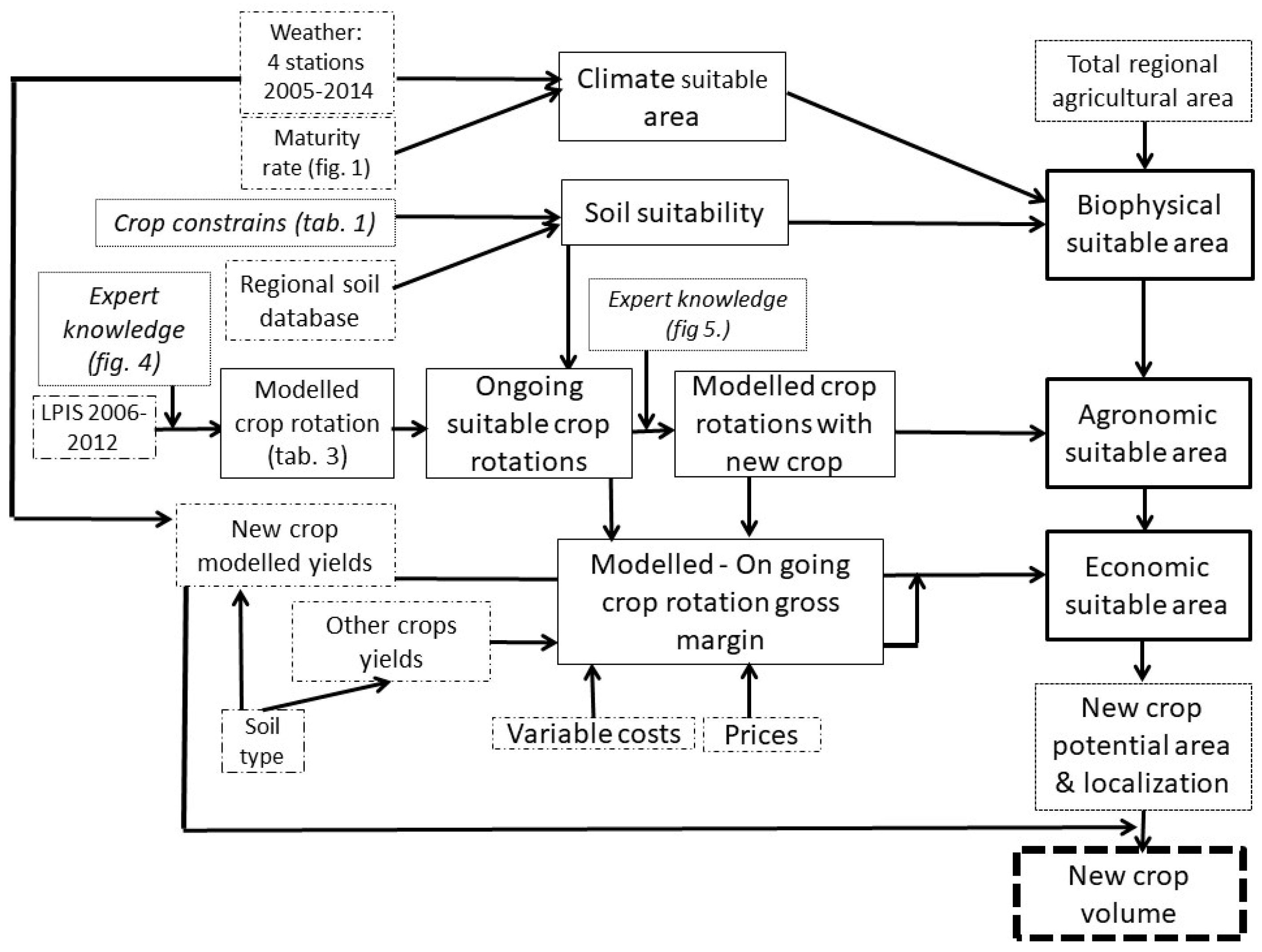
2.1. Overall Method
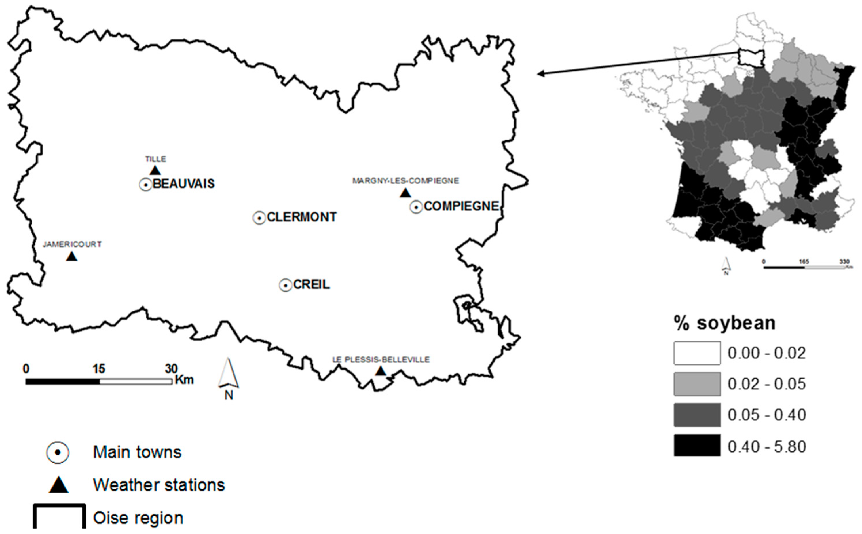
2.2. Case Study
2.3. Biophysical Suitable Areas for Soybean in the Oise Region
2.3.1. Climate Suitability
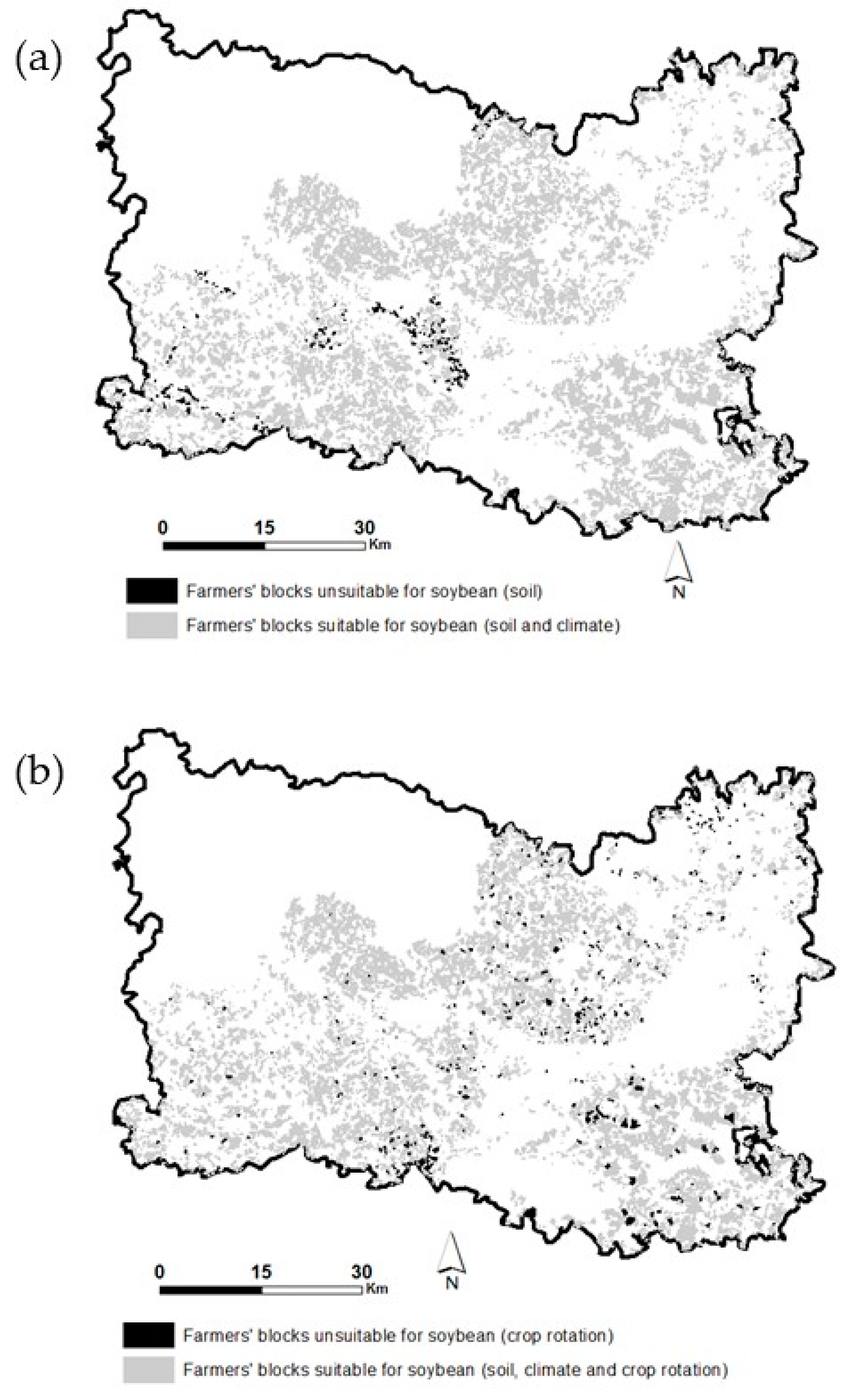
2.3.2. Soil Suitability
2.4. Suitable Areas for Soybean from an Agronomic Point of View
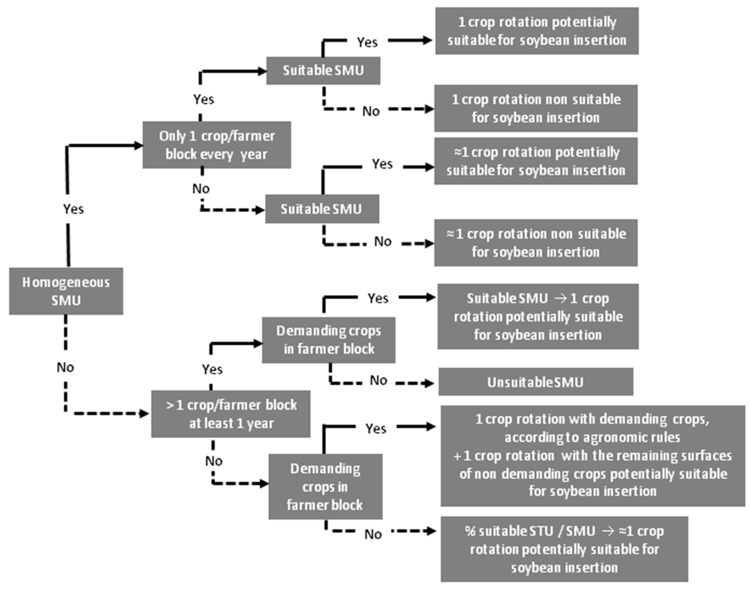
2.4.1. Modelled Crop Rotation Based on Ongoing Crop Sequences
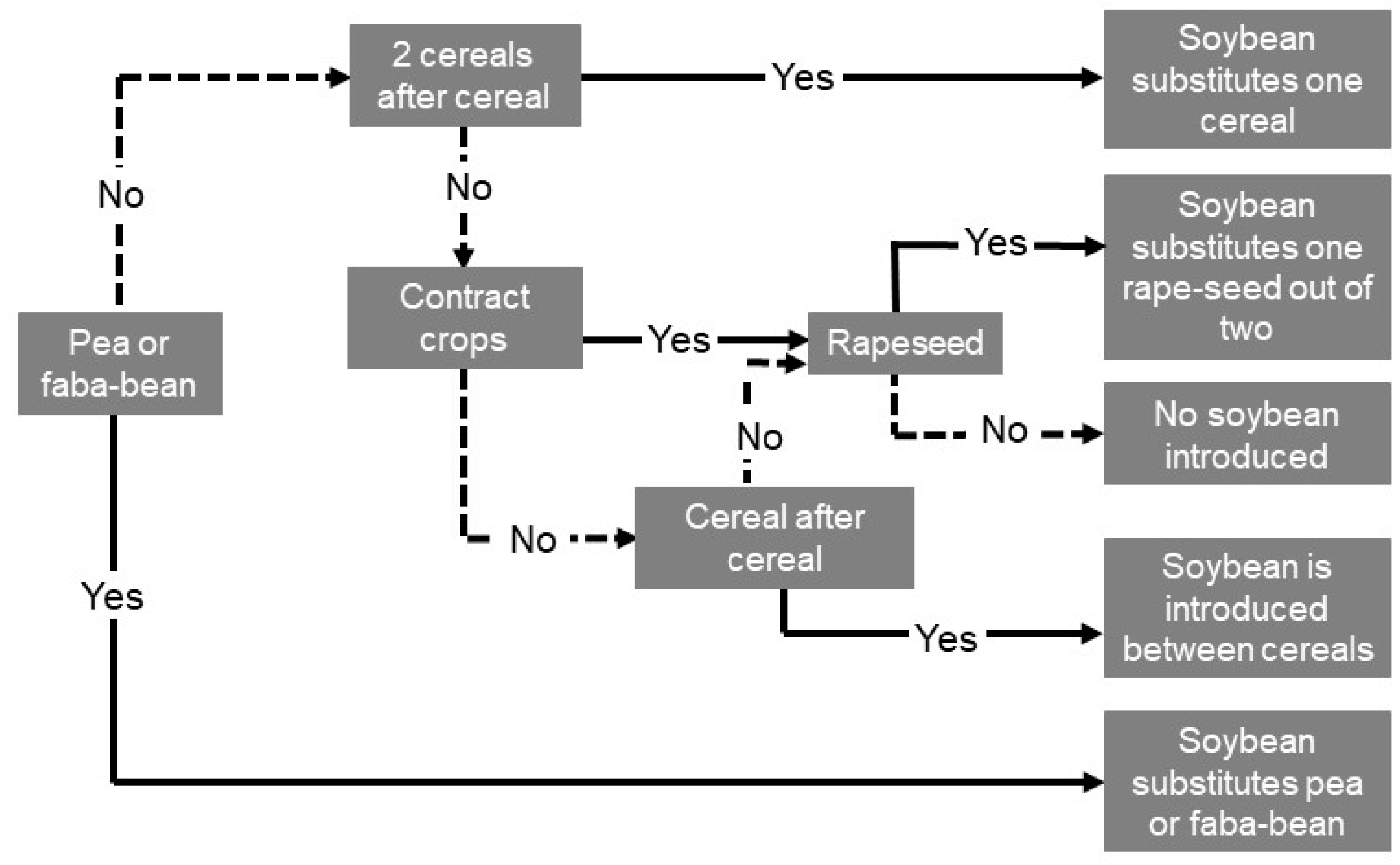
2.4.2. Re-Designed Crop Rotations with Soybean
2.5. Economic Suitable Areas for Soybean
2.6. Crops’ Yields—Soybean
2.7. Crops’ Yields—Crops Other Than Soybean
2.8. Crop Selling Prices
2.9. Variable Costs
2.10. Potential for Soybean Introduction in the Oise Region
3. Results
3.1. Suitable Climatic Area for Soybean Introduction
3.2. Soil Suitable Area for Soybean
3.3. Suitable Areas for Soybean from an Agronomic Point of View
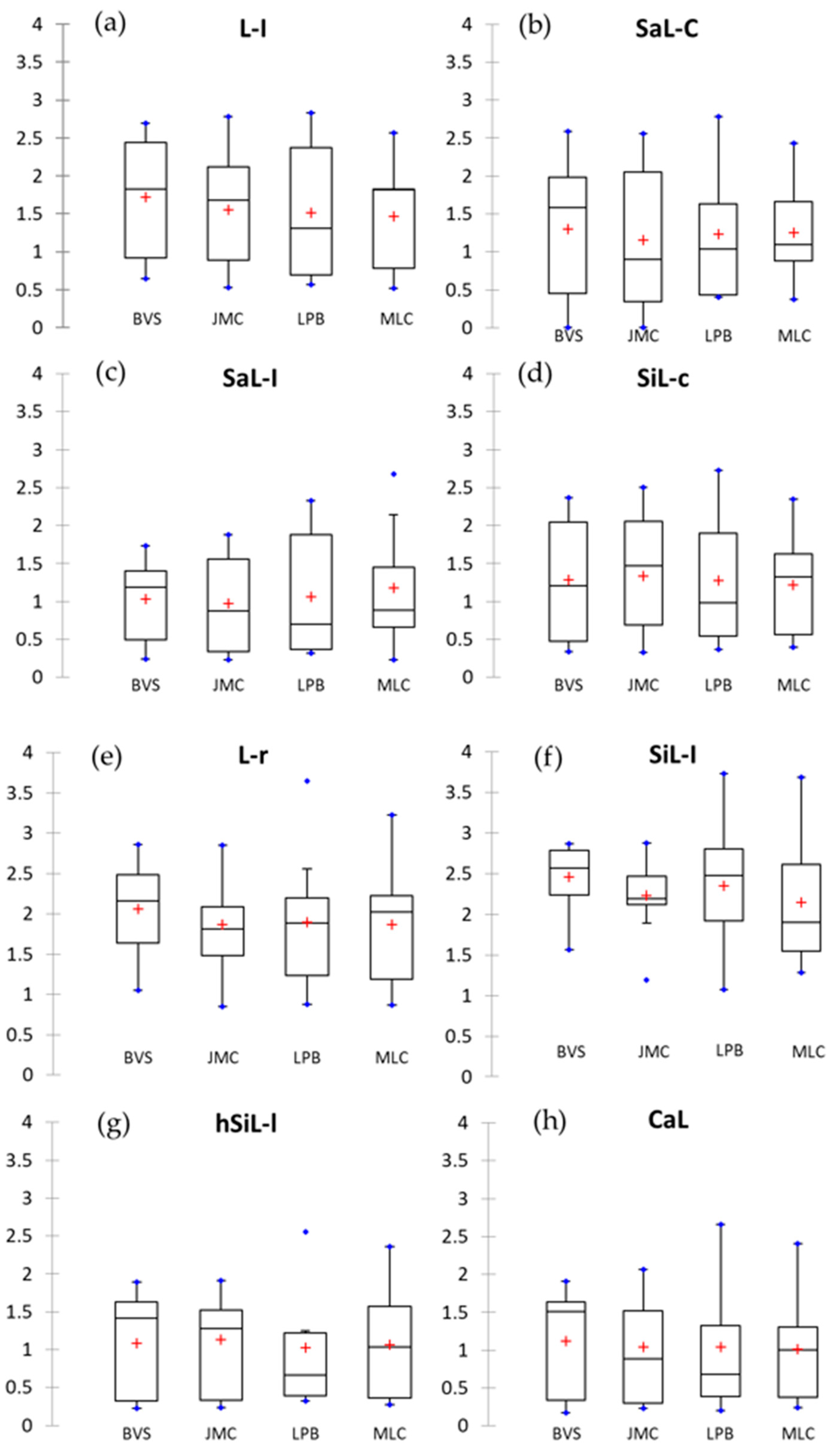
3.4. Soybean Yield Simulation
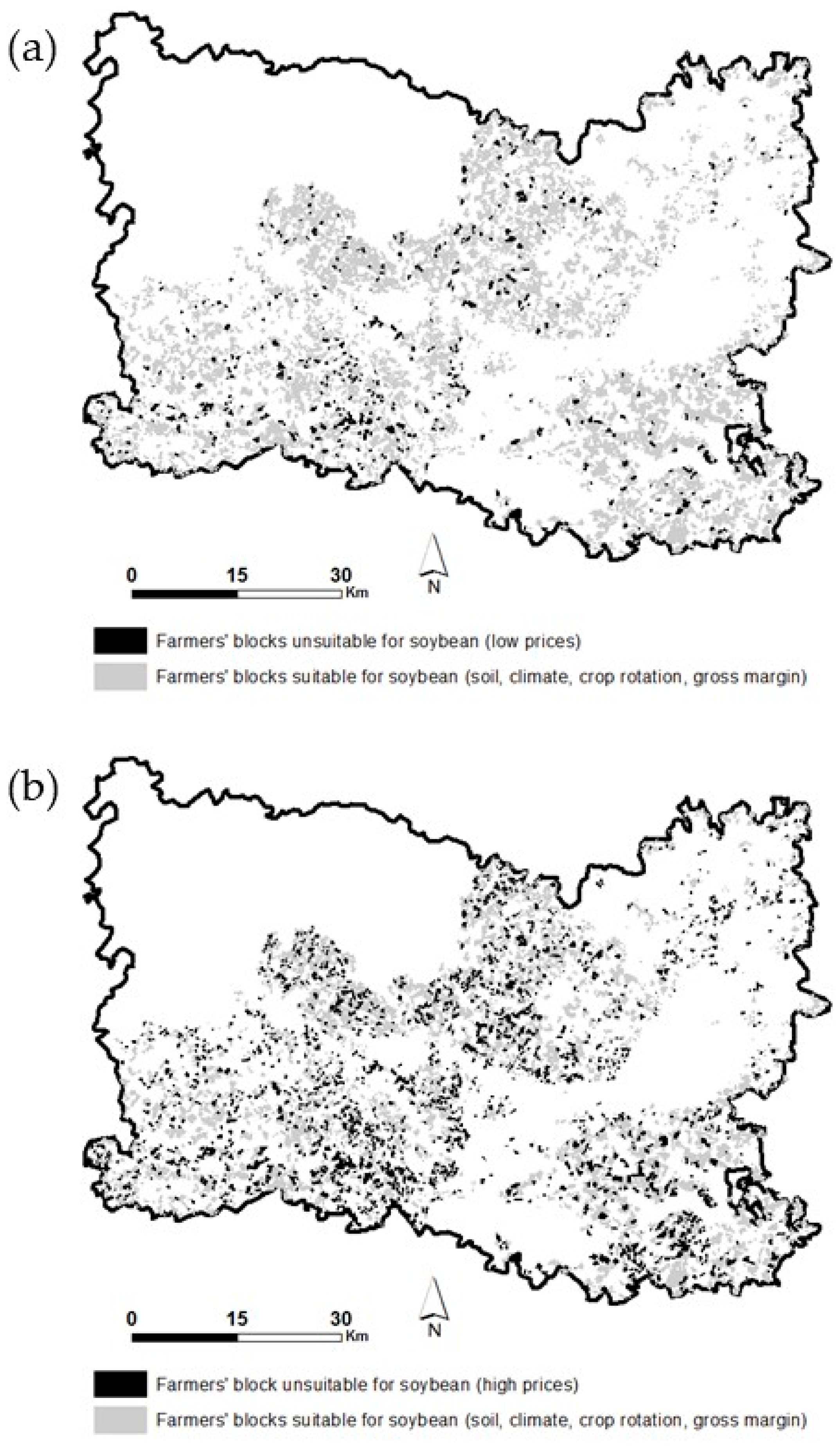
3.5. Economic Suitability for Soybean
3.6. Potential for Soybean Production in the Oise Region
4. Discussion
4.1. Uncertainty Regarding the Land Suitability Results is Highly Dependent on Assumptions on Crop Allocation, Farmers Practices and Data Availability
4.2. Barriers to the Introduction of New Crops
4.3. General Interest of the Method
5. Conclusions
Author Contributions
Funding
Acknowledgments
Conflicts of Interest
Appendix A

| Soil Ttype | SiL-l | SiL-c | SaL-l | SaL-c | CaL | hSiL-l | L-r | L-l |
|---|---|---|---|---|---|---|---|---|
| Main characteristics | Deep silt loam | Moderately deep silt loam | Moderately deep Sandy loam | Moderately deep Sandy loam | Shallow calcareous loam | Moderately deep silt loam hydromorphic | Deep loam/silt loam | Deep loam |
| Reference soil group (WRB) | luvisol | Cambisol | luvisol | cambisol | leptosol | luvisol | regosol | luvisol |
| Argi * | 17 | 24 | 10 | 18 | 14 | 21 | 25 | 15 |
| Norg | 0.12 | 0.12 | 0.12 | 0.12 | 0.12 | 0.12 | 0.12 | 0.12 |
| Profhum | 35 | 35 | 35 | 35 | 35 | 35 | 35 | 35 |
| Calc | 1 | 1 | 1 | 1 | 50 | 1 | 7 | 1 |
| pH | 7 | 7 | 7 | 7 | 8 | 7 | 7 | 7 |
| Albedo | 0.22 | 0.25 | 0.25 | 0.25 | 0.31 | 0.22 | 0.22 | 0.23 |
| q0 | 8 | 9 | 7.5 | 8 | 9 | 9 | 9 | 7 |
| Obstarac | 130 | 80 | 80 | 85 | 55 | 50 | 200 | 100 |
| Zesx | 120 | 90 | 110 | 120 | 70 | 90 | 120 | 120 |
| Epc | ||||||||
| Horizon 1 | 30 | 25 | 30 | 35 | 30 | 30 | 30 | 35 |
| Horizon 2 | 15 | 15 | 15 | 35 | 25 | 30 | 65 | 35 |
| Horizon 3 | 20 | 20 | 35 | 15 | 0 | 0 | 30 | 30 |
| Horizon 4 | 15 | 20 | 0 | 0 | 0 | 0 | 0 | 0 |
| Horizon 5 | 50 | 0 | 0 | 0 | 0 | 0 | 0 | 0 |
| HCCF | ||||||||
| Horizon 1 | 23 | 24 | 15 | 19 | 25 | 24 | 24 | 20 |
| Horizon 2 | 25.5 | 29.5 | 10.5 | 19 | 24 | 25.5 | 22.5 | 22.5 |
| Horizon 3 | 25.5 | 24 | 10.5 | 19 | 0 | 0 | 22.5 | 19 |
| Horizon 4 | 25.5 | 24 | 0 | 0 | 0 | 0 | 0 | 0 |
| Horizon 5 | 25.5 | 0 | 0 | 0 | 0 | 0 | 0 | 0 |
| HMINF | ||||||||
| Horizon 1 | 10 | 12 | 5 | 10 | 10 | 12 | 12 | 8.9 |
| Horizon 2 | 12.8 | 22 | 4 | 10 | 10 | 13 | 12 | 12.8 |
| Horizon 3 | 12.8 | 10 | 4 | 10 | 0 | 0 | 12 | 10 |
| Horizon 4 | 12.8 | 10 | 0 | 0 | 0 | 0 | 0 | 0 |
| Horizon 5 | 12.8 | 0 | 0 | 0 | 0 | 0 | 0 | 0 |
| DAF | ||||||||
| Horizon 1 | 1.4 | 1.45 | 1.4 | 1.5 | 1.2 | 1.45 | 1.45 | 1.5 |
| Horizon 2 | 1.5 | 1.45 | 1.5 | 1.6 | 1.25 | 1.5 | 1.55 | 1.55 |
| Horizon 3 | 1.5 | 1.25 | 1.5 | 1.6 | 0 | 0 | 1.55 | 1.6 |
| Horizon 4 | 1.5 | 1.25 | 0 | 0 | 0 | 0 | 0 | 0 |
| Horizon 5 | 1.5 | 0 | 0 | 0 | 0 | 0 | 0 | 0 |
| Cailloux | ||||||||
| Horizon 1 | 0 | 3 | 2 | 0 | 2 | 0 | 3 | 0 |
| Horizon 2 | 0 | 7 | 0 | 0 | 2 | 0 | 0 | 0 |
| Horizon 3 | 0 | 30 | 0 | 0 | 0 | 0 | 0 | 0 |
| Horizon 4 | 0 | 20 | 0 | 0 | 0 | 0 | 0 | 0 |
| Horizon 5 | 0 | 35 | 0 | 0 | 0 | 0 | 0 | 0 |
References
- Wezel, A.; Casagrande, M.; Celette, F.; Vian, J.F.; Ferrer, A.; Peigné, J. Agroecological practices for sustainable agriculture. A review. Agron. Sustain. Dev. 2014, 34, 1–20. [Google Scholar] [CrossRef]
- Bowen, C.R.; Hollinger, S.E. Geographic screening of potential alternative crops. Renew. Agric. Food Syst. 2004, 19, 141–151. [Google Scholar] [CrossRef]
- Isbell, F.; Adler, P.R.; Eisenhauer, N.; Fornara, D.; Kimmel, K.; Kremen, C.; Letourneau, D.K.; Liebman, M.; Polley, H.W.; Quijas, S.; et al. Benefits of increasing plant diversity in sustainable agroecosystems. J. Ecol. 2017, 105, 871–879. [Google Scholar] [CrossRef]
- Maaz, T.; Wulfhorst, J.D.; McCracken, V.; Kirkegaard, J.; Huggins, D.R.; Roth, I.; Kaur, H.; Pan, W. Economic, policy, and social trends and challenges of introducing oilseed and pulse crops into dryland wheat cropping systems. Agric. Ecosyst. Environ. 2018, 253, 177–194. [Google Scholar] [CrossRef]
- European Commission. Development of Plant Proteins in the European Union; Commission to the Council and The European Parliament: Brussels, Belgium, 2018; p. 16. [Google Scholar]
- Louhichi, K.; Ciaian, P.; Espinosa, M.; Colen, L.; Perni, A.; Paloma, S.G. Does the crop diversification measure impact EU farmers’ decisions? An assessment using an Individual Farm Model for CAP Analysis (IFM-CAP). Land Use Policy 2017, 66, 250–264. [Google Scholar] [CrossRef]
- Meynard, J.-M.; Messéan, A.; Charlier, F.; Charrier, M.; Farès, M.; Le Bail, M.; Magrini, M.-B.; Savini, I. Crop Diversification: Obstacles and Levers Study of Farms and Supply Chains; Synopsis of the study report; INRA: Paris, France, 2013. [Google Scholar]
- Leclère, M.; Loyce, C.; Jeuffroy, M.-H. Growing camelina as a second crop in France: A participatory design approach to produce actionable knowledge. Eur. J. Agron. 2018, 101, 78–89. [Google Scholar] [CrossRef]
- Rossiter, D.G. A theoretical framework for land evaluation. Geoderma 1996, 72, 165–190. [Google Scholar] [CrossRef]
- Sillero, N. What does ecological modelling model? A proposed classification of ecological niche models based on their underlying methods. Ecol. Model. 2011, 222, 1343–1346. [Google Scholar] [CrossRef]
- Rhebergen, T.; Fairhurst, T.; Zingore, S.; Fisher, M.; Oberthür, T.; Whitbread, A. Climate, soil and land-use based land suitability evaluation for oil palm production in Ghana. Eur. J. Agron. 2016, 81, 1–14. [Google Scholar] [CrossRef]
- Soltani, A.; Stoorvogel, J.J.; Veldkamp, A. Model suitability to assess regional potato yield patterns in northern Ecuador. Eur. J. Agron. 2013, 48, 101–108. [Google Scholar] [CrossRef]
- Ma, D.; Stützel, H. Prediction of winter wheat cultivar performance in Germany: At national, regional and location scale. Eur. J. Agron. 2014, 52, 210–217. [Google Scholar] [CrossRef]
- Daccache, A.; Keay, C.; Jones, R.J.A.; Weatherhead, E.K.; Stalham, M.A.; Knox, J.W. Climate change and land suitability for potato production in England and Wales: Impacts and adaptation. J. Agric. Sci. 2012, 150, 161–177. [Google Scholar] [CrossRef]
- Shabani, F.; Kumar, L.; Taylor, S. Suitable regions for date palm cultivation in Iran are predicted to increase substantially under future climate change scenarios. J. Agric. Sci. 2014, 152, 543–557. [Google Scholar] [CrossRef]
- Geerts, S.; Raes, D.; Garcia, M.; Del Castillo, C.; Buytaert, W. Agro-climatic suitability mapping for crop production in the Bolivian Altiplano: A case study for quinoa. Agric. For. Meteorol. 2006, 139, 399–412. [Google Scholar] [CrossRef]
- Mendas, A.; Delali, A. Integration of MultiCriteria Decision Analysis in GIS to develop land suitability for agriculture: Application to durum wheat cultivation in the region of Mleta in Algeria. Comput. Electron. Agric. 2012, 83, 117–126. [Google Scholar] [CrossRef]
- Ragaglini, G.; Triana, F.; Villani, R.; Bonari, E. Can sunflower provide biofuel for inland demand? An integrated assessment of sustainability at regional scale. Energy 2011, 36, 2111–2118. [Google Scholar] [CrossRef]
- Ziadat, F.M.; Sultan, K.A. Combining current land use and farmers’ knowledge to design land-use requirements and improve land suitability evaluation. Renew. Agric. Food Syst. 2011, 26, 287–296. [Google Scholar] [CrossRef]
- Debolini, M.; Marraccini, E.; Rizzo, D.; Galli, M.; Bonari, E. Mapping local spatial knowledge in the assessment of agricultural systems: A case study on the provision of agricultural services. Appl. Geogr. 2013, 42, 23–33. [Google Scholar] [CrossRef]
- Aubry, C.; Papy, F.; Capillon, A. Modelling decision-making processes for annual crop management. Agric. Syst. 1998, 56, 45–65. [Google Scholar] [CrossRef]
- Castellazzi, M.S.; Wood, G.A.; Burgess, P.J.; Morris, J.; Conrad, K.F.; Perry, J.N. A systematic representation of crop rotations. Agric. Syst. 2008, 97, 26–33. [Google Scholar] [CrossRef]
- Doré, T. L’assolement: Acception et problématiques agronomiques actuelles. Agron. Environ. Sociétés 2012, 2, 17–28. [Google Scholar]
- Chopin, P.; Blazy, J.-M.; Doré, T. A new method to assess farming system evolution at the landscape scale. Agron. Sustain. Dev. 2015, 35, 325–337. [Google Scholar] [CrossRef]
- Levavasseur, F.; Martin, P.; Bouty, C.; Barbottin, A.; Bretagnolle, V.; Thérond, O.; Scheurer, O.; Piskiewicz, N. RPG Explorer: A new tool to ease the analysis of agricultural landscape dynamics with the Land Parcel Identification System. Comput. Electron. Agric. 2016, 127, 541–552. [Google Scholar] [CrossRef]
- Murgue, C.; Therond, O.; Leenhardt, D. Hybridizing local and generic information to model cropping system spatial distribution in an agricultural landscape. Land Use Policy 2016, 54, 339–354. [Google Scholar] [CrossRef]
- Barbottin, A.; Bouty, C.; Martin, P. Using the French LPIS database to highlight farm area dynamics: The case study of the Niort Plain. Land Use Policy 2018, 73, 281–289. [Google Scholar] [CrossRef]
- Sagris, V.; Wojda, P.; Milenov, P.; Devos, W. The harmonised data model for assessing Land Parcel Identification Systems compliance with requirements of direct aid and agri-environmental schemes of the CAP. J. Environ. Manag. 2013, 118, 40–48. [Google Scholar] [CrossRef]
- Leteinturier, B.; Herman, J.L.; Longueville, F.; de Quintin, L.; Oger, R. Adaptation of a crop sequence indicator based on a land parcel management system. Agric. Ecosyst. Environ. 2006, 112, 324–334. [Google Scholar] [CrossRef]
- Xiao, Y.; Mignolet, C.; Mari, J.-F.; Benoît, M. Modeling the spatial distribution of crop sequences at a large regional scale using land-cover survey data: A case from France. Comput. Electron. Agric. 2014, 102, 51–63. [Google Scholar] [CrossRef]
- Metzger, M.J.; Bunce, R.G.H.; Jongman, R.H.G.; Mücher, C.A.; Watkins, J.W. A climatic stratification of the environment of Europe. Glob. Ecol. Biogeogr. 2005, 14, 549–563. [Google Scholar] [CrossRef]
- CA Oise. Présentation Des Systèmes D’exploitation Agricole De Picardie; Chambre d’Agriculture de l’Oise: Beauvais, France, 2010; p. 436. [Google Scholar]
- Plan Ecophyto II; Ministère de L’Agriculture et de L’Alimentation: Paris, France, 2015; p. 67.
- Agreste. Memento De La Statistique Agricole. Direction Régionale De L’Alimentation, De L’Agriculture Et De La Forêt; Service Régional de L’Information Statistique Et Economique: Paris, France, 2016; p. 26. [Google Scholar]
- Terres Inovia. Synthèse Soja Réseau Terres Inovia; Résultats Des Variétés Issues Du Catalogue Français: Paris, France, 2016; p. 5. [Google Scholar]
- Ku, Y.S.; Au-Yeung, W.K.; Ying, Y.L.; Li, M.W.; Wen, C.Q.; Liu, X.; Lam, H.M. Drought stress and tolerance in soybean. In A Comprehensive Survey of International Soybean Research—Genetics, Physiology, Agronomy and Nitrogen Relationships; James, E., Ed.; IntechOpen: London, UK, 2013; pp. 209–238. [Google Scholar] [CrossRef]
- Sentelhas, P.C.; Battisti, R.; Câmara, G.M.S.; Farias, J.R.B.; Hampf, A.C.; Nendel, C. The soybean yield gap in Brazil—Magnitude, causes and possible solutions for sustainable production. J. Agric. Sci. 2015, 153, 1394–1411. [Google Scholar] [CrossRef]
- Aper, J.; De Clercq, H.; Baert, J. Agronomic characteristics of early-maturing soybean and implications for breeding in Belgium. Plant Genet. Resour. 2016, 14, 142–148. [Google Scholar] [CrossRef]
- King, D.; Stengel, P.; Jamagne, M.; Le Bas, C.; Arrouays, D. Soil Mapping and Soil Monitoring: State of Progress and Use in France; Jones, Ed.; Soil Resources of Europe, European Soil Bureau, Institute of Environmental Sustainability, JRC: Ispra, Italy, 2005; p. 433. [Google Scholar]
- Arrouays, D.; Hardy, R.; Schnebelen, N.; Le Bas, C.; Eimberck, M.; Roque, J.; Grolleau, E.; Pelletier, A.; Doux, J.; Lehmann, S.; et al. Le programme Inventaire Gestion et Conservation des Sols de France. Etude Gest. Sols 2004, 11, 187–197. [Google Scholar]
- Inskeep, W.; Bloom, P.R. Effects of Soil Moisture on Soil pCO2, Soil Solution Bicarbonate, and Iron Chlorosis in Soybeans 1. SSSAJ 1986, 50, 946–952. [Google Scholar] [CrossRef]
- Rodrigues, T.R.; Casaroli, D.; Evangelista, A.W.P.; Alves Júnior, J. Water availability to soybean crop as a function of the least limiting water range and evapotranspiration1. Pesqui. Agropecuária Trop. 2017, 47, 161–167. [Google Scholar] [CrossRef]
- Oosterhuis, D.M.; Scott, H.D.; Hampton, R.E.; Wullschleger, S.D. Physiological responses of two soybean [Glycine max (L.) Merr] cultivars to short-term flooding. Environ. Exp. Bot. 1990, 30, 85–92. [Google Scholar] [CrossRef]
- EEA. Corine Land Cover Technical Guidelines; European Environmental Agency: Copenhagen, Denmark, 2007. [Google Scholar]
- Zimmermann, J.; González, A.; Jones, M.B.; O’Brien, P.; Stout, J.C.; Green, S. Assessing land-use history for reporting on cropland dynamics—A comparison between the Land-Parcel Identification System and traditional inter-annual approaches. Land Use Policy 2016, 52, 30–40. [Google Scholar] [CrossRef]
- Brisson, N.; Mary, B.; Ripoche, D.; Jeuffroy, M.H.; Ruget, F.; Nicoullaud, B.; Gate, P.; Devienne-Barret, F.; Antonioletti, R.; Durr, C.; et al. STICS: A generic model for the simulation of crops and their water and nitrogen balances. I. Theory and parameterization applied to wheat and corn. Agronomie 1998, 18, 311–346. [Google Scholar] [CrossRef]
- Brisson, N.; Ruget, F.; Gate, P.; Lorgeou, J.; Nicoullaud, B.; Tayot, X.; Plenet, D.; Jeuffroy, M.-H.; Bouthier, A.; Ripoche, D.; et al. STICS: A generic model for simulating crops and their water and nitrogen balances. II. Model validation for wheat and maize. Agronomie 2002, 22, 69–92. [Google Scholar] [CrossRef]
- Jégo, G.; Pattey, E.; Bourgeois, G.; Morrison, M.J.; Drury, C.F.; Tremblay, N.; Tremblay, G. Calibration and performance evaluation of soybean and spring wheat cultivars using the STICS crop model in Eastern Canada. Field Crop. Res. 2010, 117, 183–196. [Google Scholar] [CrossRef]
- Guichard, L.; Bockstaller, C.; Loyce, C.; Makowski, D. PERSYST, a cropping system model based on local expert knowledge. In Proceedings of the Agro 2010 the XIth ESA Congress; Wery, J., Shili-Touzi, I., Perrin, A., Eds.; Agropolis International Editions: Motpellier, France, 2010; pp. 827–828. [Google Scholar]
- Arvalis-Institut du végétal. UNIP Pois. In Quoi De Neuf Protéagineux; Editions Arvalis: Flers, France, 2012; pp. 56–62. [Google Scholar]
- Rieu, C.; Doucet, R.; Seguin, B.; Jouy, L.; Vacher, C.; Bordes, J.P.; Viaux, P. Blé sur blé: Techniques et enjeux. Perspect. Agric. 2000, 258, 26–31. [Google Scholar]
- CA Oise. Assolement & Stratégie, Récolte 2015; Chambre d’Agriculture de l’Oise: Beauvais, France, 2015; p. 22. [Google Scholar]
- COMIFER. Calcul de la Fertilisation Azotée-Guide Méthodologique Pour L’établissement Des Prescriptions Locales. Cultures Annuelles et Prairies; COMité Français d’Etude et de développement de la FERtilisation raisonnée: Paris, France, 2013; p. 159. [Google Scholar]
- Ansel, O.; Epinat, V.; Scheurer, O. Guide Agronomique Des Sols Du Département De L’Oise. ISAB/Conseil Général De L’Oise/Chambre d’Agriculture de l’Oise. Available online: http://www.chambres-agriculture-picardie.fr/menus-horizontaux/oise/la-chambre-dagriculture-de-loise/outils-pratiques/guide-des-sols.html (accessed on 16 December 2019).
- Peregrine, E.K.; Sprau, G.L.; Cremeens, C.R.; Nelson, R.L.; Orf, J.H.; Thomas, D.A. Evaluation of the USDA Soybean Germplasm Collection: Maturity Groups 000-IV (PI 578371-PI612761); Technical Bulletin; U.S. Department of Agriculture: Washington, DC, USA, 2008; p. 155.
- Benoît, M.; Rizzo, D.; Marraccini, E.; Moonen, A.C.; Galli, M.; Lardon, S.; Rapey, H.; Thenail, C.; Bonari, E. Landscape agronomy: A new field for addressing agricultural landscape dynamics. Landsc. Ecol. 2012, 27, 1385–1394. [Google Scholar] [CrossRef]
- Castellazzi, M.S.; Matthews, J.; Angevin, F.; Sausse, C.; Wood, G.A.; Burgess, P.J.; Brown, I.; Conrad, K.F.; Perry, J.N. Simulation scenarios of spatio-temporal arrangement of crops at the landscape scale. Environ. Model. Softw. 2010, 25, 1881–1889. [Google Scholar] [CrossRef]
- Voisin, A.-S.; Guéguen, J.; Huyghe, C.; Jeuffroy, M.-H.; Magrini, M.-B.; Meynard, J.-M.; Mougel, C.; Pellerin, S.; Pelzer, E. Legumes for feed, food, biomaterials and bioenergy in Europe: A review. Agron. Sustain. Dev. 2014, 34, 361–380. [Google Scholar] [CrossRef]
- Zander, P.; Amjath-Babu, T.S.; Preissel, S.; Reckling, M.; Bues, A.; Schläfke, N.; Kuhlman, T.; Bachinger, J.; Uthes, S.; Stoddard, F.; et al. Grain legume decline and potential recovery in European agriculture: A review. Agron. Sustain. Dev. 2016, 36, 26. [Google Scholar] [CrossRef]
- Magrini, M.-B.; Anton, M.; Cholez, C.; Corre-Hellou, G.; Duc, G.; Jeuffroy, M.-H.; Meynard, J.-M.; Pelzer, E.; Voisin, A.-S.; Walrand, S. Why are grain-legumes rarely present in cropping systems despite their environmental and nutritional benefits? Analyzing lock-in in the French agrifood system. Ecol. Econ. 2016, 126, 152–162. [Google Scholar] [CrossRef]
- Zimdahl, R.L. Fundamentals of Weed Science, 3rd ed.; Elsevier: Amsterdam, The Netherlands, 2007; ISBN 978-0-12-372518-9. [Google Scholar]
- Boulch, G.; Djemel, A.; Lange, B. Evaluation of the Potential Adaptation of Soybean (Glycine Max L.) to Northern France Using Crop Modeling Simulations. In Proceedings of the ICROPM2020—Crop Modelling for the Future. Book of Abstract, Second International Crop Modelling Symposium, Montpellier, France, 3–5 February 2020; pp. 371–372. Available online: https://www.alphavisa.com/icropm/2020/documents/iCROPM2020-Book-of-Abstracts.pdf (accessed on 19 February 2020).
- Boettinger, J.; Howell, D.; Moore, A.; Hartemink, A.; Kienast-brown, S. Digital Soil Mapping: Bridging Research, Environmental Application, and Operation; Springer: Dordrecht, The Netherlands; Heidelberg, Germany; London, UK; New York, NY, USA, 2010. [Google Scholar]
- Martínez-Casasnovas, J.A.; Martín-Montero, A.; Auxiliadora Casterad, M. Mapping multi-year cropping patterns in small irrigation districts from time-series analysis of Landsat TM images. Eur. J. Agron. 2005, 23, 159–169. [Google Scholar] [CrossRef]
- Rötter, R.P.; Palosuo, T.; Kersebaum, K.C.; Angulo, C.; Bindi, M.; Ewert, F.; Ferrise, R.; Hlavinka, P.; Moriondo, M.; Nendel, C.; et al. Simulation of spring barley yield in different climatic zones of Northern and Central Europe: A comparison of nine crop models. Field Crop. Res. 2012, 133, 23–36. [Google Scholar] [CrossRef]


| STU Suitability Class | Agronomic Constraints |
|---|---|
| Unsuitable | Carbonate > 15% or stone/gravel > 15% or Soil-AWC < 100 mm |
| Suitable | Carbonate < 15% and stone/gravel < 15% and 100 < Soil-AWC < 170 mm |
| Highly suitable | Carbonate < 15% and stone/gravel < 15% and Soil-AWC > 170 mm |
| SMU Suitability Class | Characteristics |
|---|---|
| Homogeneous-unsuitable | 100% unsuitable |
| Homogeneous-suitable | 100% suitable |
| Homogeneous-highly suitable | 100% highly suitable |
| Heterogeneous | Partly unsuitable and partly suitable |
| Heterogeneous-suitable | Partly suitable and partly highly suitable |
| Crop | Light, High AWC | Light Medium/Low AWC | Chalky Low AWC | Clayey High AWC | Clayey, Medium AWC | Loamy, High AWC | Loamy, Medium AWC |
|---|---|---|---|---|---|---|---|
| Winter soft wheat | 8.4 | 7.2 | 8.3 | 7.6 | 8.2 | 9.7 | 9.2 |
| Winter barley | 8.5 | 7.2 | 8.0 | 7.5 | 8.0 | 9.2 | 8.8 |
| Summer barley | 6.5 | 5.4 | 5.7 | 5.1 | 6.5 | 7.3 | 6.5 |
| Rape seed | 4.0 | 3.4 | 3.5 | 3.4 | 3.5 | 45 | 4.3 |
| Sugar beet | 70.0 | 70.0 | 80.0 | 95.0 | 95.0 | 105.0 | 105.0 |
| Grain corn | 8.3 | 8.5 | - | - | 8.5 | 10.3 | 9.2 |
| Legumes | 4.8 | 4.4 | 4.1 | - | 5.0 | 5.5 | 5.0 |
| Sunflower | 2.0 | 1.5 | 2.2 | 2.5 | 2.5 | 3.0 | 2.7 |
| Linseed | 2.6 | 2.6 | 2.1 | 2.2 | 2.5 | 2.8 | 2.5 |
| Flaxseed | 6.5 | 5.1 | 4.8 | - | - | 6.8 | 6.1 |
| Crop | Variable Costs (€/ha) | High Selling Price (€/t) | Low Selling Price (€/t) |
|---|---|---|---|
| Wheat | 382 | 190 | 150 |
| Barley | 288 | 190 | 140 |
| Legume | 418 | 220 | 170 |
| Rape seed | 329 | 440 | 300 |
| Industrial vegetables | Fixed (contract crops) | ||
| Set-aside | 0 | 0 | 0 |
| Soybean | 522 | 450 | 350 |
| Oat | 240 | 180 | 140 |
| Sugar Beet | Fixed (contract crop) | ||
| Flaxseed | 408 | 270 | 180 |
| Corn | 452 | 190 | 140 |
| Linseed | 300 | 490 | 380 |
| Sunflower | 270 | 460 | 325 |
| Weather Stations | Number of Farmer Blocks | Total Farmer Block Area (ha) | % of the Suitable Climatic Agricultural Area |
|---|---|---|---|
| Jaméricourt | 1614 | 13,898 | 17% |
| Le Plessis-Belleville | 1575 | 18,868 | 23% |
| Margny-lès-Compiègne | 5346 | 29,869 | 36% |
| Tillé | 3786 | 19,748 | 24% |
| Soil Type | Number of Farmer Blocks | Total Farmer Blocks’ Area (ha) | % on the Climatically Suitable Area |
|---|---|---|---|
| Chalky, high AWC | 347 | 2139 | 2.6% |
| Chalky, low AWC * | 545 | 3054 | 3.7% |
| Clayey, high AWC | 1790 | 7903 | 9.6% |
| Clayey, medium/low AWC | 221 | 1416 | 1.7% |
| Light, high AWC | 14 | 48 | <0.01% |
| Light, medium/low AWC | 1446 | 8902 | 10.8% |
| Loamy, high AWC | 5370 | 42,624 | 51.7% |
| Loamy, medium/low AWC | 2606 | 16,370 | 19.8% |
| Agronomic Introduction Rule | Number of Farmers’ Blocks | Total Blocks Area (ha) | Rate for Different Soil Type Area (%) | ||||||
|---|---|---|---|---|---|---|---|---|---|
| Light | Chalky | Clayey | Loamy | ||||||
| High AWC | Medium/Low AWC | High AWC | High AWC | Medium AWC | High AWC | Medium AWC | |||
| One cereal over 2 cereals | 3171 | 22,597 | 0 | 13.1 | 2.1 | 0 | 2.4 | 57.5 | 24.7 |
| One cereal over 3 cereals | 1290 | 5198 | 0.2 | 18.1 | 3.5 | 0 | 1.9 | 47.8 | 28.3 |
| Between two rape seeds | 14 | 110 | 0 | 6.4 | 0 | 0 | 0 | 84.5 | 9.1 |
| Grain legumes | 6482 | 47,578 | 0 | 10.1 | 3.1 | 11.3 | 15.8 | 51.4 | 19.0 |
| No soybean | 440 | 3304 | 0.1 | 5.4 | 0.4 | 6.8 | 0.6 | 77.8 | 8.0 |
| Variability of the Gross Margin after Soybean Introduction | Farmers’ Blocks | Total Area (ha) | Area Rate for Different Soybean Introduction Rules (%) | ||||
|---|---|---|---|---|---|---|---|
| One Cereal over 2 Cereals | One Cereal over 3 Cereals | Between two Rape Seeds | Grain Legumes | ||||
| Low price | Very suitable | 5739 | 46,417 | 81% | 2% | 0% | 17% |
| Suitable | 3902 | 19,691 | 72% | 20% | 0% | 7% | |
| Unsuitable | 528 | 5354 | 89% | 10% | 1% | 0% | |
| High price | Very suitable | 5721 | 46,079 | 10% | 2% | 0% | 88% |
| Suitable | 1748 | 8711 | 40% | 43% | 0% | 17% | |
| Unsuitable | 2700 | 16,672 | 94% | 5% | 1% | 0% | |
| Crops’ Proportion in the Crop Sequence | Hypothesis on the Crop Rotation | Ongoing Crop Rotation | Applied Agronomic Rule | Soybean Return Period | Effect of Short Rotation Hypothesis on Soybean Area |
|---|---|---|---|---|---|
| C: 50% R: 17% M: 17% Set aside: 16% | Long: 5 years | R C M C C | Soybean substitutes one R out of two | 10 years | −25% |
| Short: 2 rotations of 2 and 3 years | ½ R C ½ M C C | Soybean substitutes one R out of two | 4 years on half area * | ||
| C: 60% R: 20% M: 10% OS: 10% | Long: 10 years | M C OS C C R C R C C | Soybean substitutes one R out of two | 10 years | +25% |
| Short: 2 rotations of 5 years | ½ R C R C C ½ OS C C M C | Soybean is inserted between two C | 6 years on half area * | ||
| C: 50% R: 6% SB: 17% Pt: 7% M: 10% Set aside: 8% | Long: 12 years | M C Pt C SB C SB C R C SB C | Soybean substitutes one R out of two | 24 years | No change |
| Short: 2 rotations of 6 years | ½ Pt C SB C SB C ½ R C M C SB C | Soybean substitutes one R out of two | 24 years |
© 2020 by the authors. Licensee MDPI, Basel, Switzerland. This article is an open access article distributed under the terms and conditions of the Creative Commons Attribution (CC BY) license (http://creativecommons.org/licenses/by/4.0/).
Share and Cite
Marraccini, E.; Gotor, A.A.; Scheurer, O.; Leclercq, C. An Innovative Land Suitability Method to Assess the Potential for the Introduction of a New Crop at a Regional Level. Agronomy 2020, 10, 330. https://doi.org/10.3390/agronomy10030330
Marraccini E, Gotor AA, Scheurer O, Leclercq C. An Innovative Land Suitability Method to Assess the Potential for the Introduction of a New Crop at a Regional Level. Agronomy. 2020; 10(3):330. https://doi.org/10.3390/agronomy10030330
Chicago/Turabian StyleMarraccini, Elisa, Alicia Ayerdi Gotor, Olivier Scheurer, and Christine Leclercq. 2020. "An Innovative Land Suitability Method to Assess the Potential for the Introduction of a New Crop at a Regional Level" Agronomy 10, no. 3: 330. https://doi.org/10.3390/agronomy10030330
APA StyleMarraccini, E., Gotor, A. A., Scheurer, O., & Leclercq, C. (2020). An Innovative Land Suitability Method to Assess the Potential for the Introduction of a New Crop at a Regional Level. Agronomy, 10(3), 330. https://doi.org/10.3390/agronomy10030330