Article

Combined Use of Multi-Temporal Landsat-8 and Sentinel-2 Images for Wheat Yield Estimates at the Intra-Plot Spatial Scale

1
Centre d’Études Spatiales de la BIOsphère (CESBIO), University of Toulouse, CNES/CNRS/INRAE/IRD/UPS, 41 Allée Jules Guesde, 31000 Toulouse, France
2
IUT Paul Sabatier, 24 rue d’Embaquès, 32000 Auch, France
*
Author to whom correspondence should be addressed.
Agronomy 2020, 10(3), 327; https://doi.org/10.3390/agronomy10030327
Submission received: 12 February 2020 / Revised: 21 February 2020 / Accepted: 24 February 2020 / Published: 28 February 2020
(This article belongs to the Special Issue Remote Sensing of Agricultural Monitoring)

Abstract

:
The objective of this study is to address the capabilities of multi-temporal optical images to estimate the fine-scale yield variability of wheat, over a study site located in southwestern France. The methodology is based on the Landsat-8 and Sentinel-2 satellite images acquired after the sowing and before the harvest of the crop throughout four successive agricultural seasons, the reflectance constituting the input variables of a statistical algorithm (random forest). The best performances are obtained when the Normalized Difference Vegetation Index (NDVI) is combined with the yield maps collected during the crop rotation, the agricultural season 2014 showing the lower level of performances with a coefficient of determination (R2) of 0.44 and a root mean square error (RMSE) of 8.13 quintals by hectare (q.h−1) (corresponding to a relative error of 12.9%), the three other years being associated with values of R2 close or upper to 0.60 and RMSE lower than 7 q.h−1 (corresponding to a relative error inferior to 11.3%). Moreover, the proposed approach allows estimating the crop yield throughout the agricultural season, by using the successive images acquired from the sowing to the harvest. In such cases, early and accurate yield estimates are obtained three months before the end of the crop cycle. At this phenological stage, only a slight decrease in performance is observed compared to the statistic obtained just before the harvest.

1. Introduction

Over the last 50 years, the world production of wheat has increased with a positive trend of around 8.7 million tons per year (value derived from the statistics of [1]). The maximal surface allocated to wheat was reached in the 1980s with 239 million hectares. With actual values higher than 200 million hectares, wheat is the world’s most abundant crop in terms of harvested area. In France, one-fifth of the useful agricultural surface is dedicated to the cultivation of wheat [2]. In this context, spatial information delivered by satellite missions represents unique opportunities, to assist management decisions in precision agriculture.
Numerous previous studies have shown the contribution of satellite imagery to wheat crop monitoring. The topics covered are diverse, ranging from land use to monitoring parameters related to the photosynthetic status of vegetation, to estimating height or biomass, or even detecting areas of lodging or inverting top surface moisture throughout the growing cycle [3,4,5,6,7]. These studies are based on a wide variety of satellite missions, characterized by sensors operating in different wavelength domains (i.e., visible, near and medium infrared, microwave) and delivering different types of products with a specific time frequency and spatial resolution. All these specificities determine the possibilities of crop monitoring, most of the work being carried out on the basis of optical data, often using regular acquisitions of medium or high spatial resolution images. These time series allow yields to be estimated and production mapped in most cases at the end of the agricultural season and at spatial scales ranging from the agricultural region (by using medium-resolution images to cover areas of several tens of km2) to the plot scale (by averaging information acquired at high spatial resolution over several hectares) [8,9,10,11,12]. The methods used are then diverse, ranging from simple empirical relationships (based on vegetation indices derived from reflectance [13,14,15]) to the assimilation of biophysical parameters (such as the leaf area index or the fraction of absorbed photosynthetically active radiation, derived from optical images by inversion of a radiative transfer model) in agro-meteorological models [16,17,18], or the use of different statistical algorithms (e.g., artificial neural network, partial least squares regression, support vector machine or random forest [19,20,21,22]). The latter approach has the advantage of obtaining high performance, particularly in a multi-factorial context, but it is conditioned by the availability of data (particularly access to field truths), which often constrains the possibilities of implementation (i.e., difficulty of independent calibration and validation procedures) and limits the representativeness of the algorithms.
Nevertheless, several on-going satellite missions provide images allowing monitoring the intra-plot variability of crop status, spatial scale consistent with the recent advances in yield sensors onboard harvesting machines. Such sensors allow accessing numerous valuable discrete information that is merged when using yield data collected at the plot spatial scale. The proposed study is part of this context, with the objective of estimating the intra-plot variability of wheat yields by combining satellite acquisitions performed by Landsat-8 and Sentinel-2A and taking advantage of the yields measured during previous or past crop rotation. Ground data collected by sensors onboard harvesting machines are described in Section 2, together with high spatial resolution images. The proposed approach is based on random forest, considering reflectance as predictive variables alone or with previous or past observations, and crop yields as target (Section 3). The results are analyzed and discussed in Section 4 and Section 5, respectively, focusing on the overall statistical performances obtained for four successive agricultural seasons and showing one example of a yield map.

2. Materials

2.1. Study Site

The study area is located in southwestern France in Gers County. Surrounded by valleys, the territory is characterized by a great diversity of landscapes and types of soil comprising ustic luvisols, limestone, clay-limestone or more sandy soils. The county is subject to oceanic and Mediterranean climatic influences, with a precipitation regime spatially and annually variable. The useful agricultural area covers 71% of the territory (or 447,223 ha), being mainly dedicated to the cultivation of seasonal crops (cereals for 44.5% or oleaginous and proteinaceous for 24%) or forage crops and evergreen surfaces for 19% [2]. The present paper focuses on the main cultivated crops in Gers County, wheat, for which the agricultural season delineated by the sowing and harvesting periods is observed from autumn to summer of the following year, respectively.

2.2. Intra-Plot Yield Data

The yields of wheat were collected during four successive agricultural seasons (2014 to 2017) over 10 or 12 field plots, depending on the considered year (Figure 1). Their sizes ranged from 3.2 to 28.6 hectares, representing an amount of more than 500 hectares considering the period of the study. The plots selected for this study had the particularity of being dedicated to the cultivation of wheat every 2 years. Consequently, for the agricultural seasons 2014 and 2016, the yields were collected on the same 10 plots, and in 2015 and 2017, the same 12 plots were surveyed. Descriptive statistics (i.e., means and standard deviations) were derived at the plot scale and presented together with the values of correlation for the following rotations: 2014–2016 and 2015–2017 (in the remainder of the article, these pairs of years are referred to as “pair years”). The mean values of yield ranged from 41.9 to 67.8 quintals by a hectare (q.h−1), showing a variability depending on the considered plot, as evidenced by the coefficients of variation (CV = 100 × standard deviation/mean) ranging from 11.2% to 32.1%. A maximal difference of ~8.5 q.ha−1 was observed between the highest and lowest productive years (i.e., difference between 2015 and 2017 agricultural season, showing a value of 58.9 to 50.4 q.ha−1 on average). The collected yields appeared consistent with values observed in Gers County, ranging from 38 to 65 q.ha−1 according to the statistics presented by the French ministry of agriculture and food since the 2000s.
The correlations between “pair years” ranged from 0.39 to 0.78 and 0.51 to 0.81 for the rotations 2014–2016 and 2015–2017, respectively (Figure 1). The high correlation values were representative of the persistence of spatial patterns in the considered plots. The plots F7 for the rotations 2015–2017 illustrated such behavior, with a high correlation associated with a different distribution of yield values. At the opposite, the plot F6 for the rotations 2014–2016 shows a close distribution of values with low correlation, meaning that the high and low productive zones were observed in different locations of the plot.
The yield values were derived from the data collected by the surveying harvesting machine with the GPS system on track mode. The yield measurements collected by the machine were associated with a position in space. In addition to the mass of the grain flow, the width of the cutting bar, the distance traveled and the moisture content of the grain were also collected. For each measurement, the area matching with the mass of the grain flow was derived by multiplying the width of the cutting bar and the distance traveled. The value of the harvested yield was computed as the mass of the grain flow divided by the area. Finally, dry yields were last calculated by accounting for the humidity of grain. All the measurements performed in a pixel with a spatial resolution of 30 m were aggregated, avoiding the extreme values (i.e., average plus three sigma or 99.7% of the values). Those maps of yields constitute the targeted variable of the statistical algorithm.

2.3. Satellite Data

The satellite images acquired during the four agricultural seasons are presented in Table 1. From October 2013 to July 2017, an amount of 52 high spatial resolution images was provided by Landsat-8 (12, 14 and 7 images, in 2014, 2015 and 2016) and Sentinel-2 (7 and 12 images, in 2016 and 2017). From 12 to 14 regular acquisitions were available for the monitoring of wheat, from the sowing to the harvest of the crop. The most important characteristics of the satellite images are presented below (Section 2.3.1 and Section 2.3.2) together with the processing steps (Section 3.1).

2.3.1. Sentinel-2A Data

Sentinel-2A is a European satellite that was launched in June 2015 [23]. This satellite has a multispectral imager that provides images in thirteen spectral bands ranging from the visible to the short-wavelength infrared. The images are characterized by a spatial resolution of 10 m for four wavelengths (490, 560, 665 and 842 nm) and 20 m for six wavelengths (705, 740, 783, 865, 1610 and 2190 nm) and of 60 m for three wavelengths (443, 945 and 1380 nm).

2.3.2. Landsat-8 Data

Landsat-8 is an American satellite that was launched in February 2013 [24]. This satellite carries the Operational Land Imager and the thermal infrared sensor which operate in spectral bands ranging from the visible to the thermal wavelengths. The images consist of one panchromatic band characterized by a spatial resolution of 10 m, two thermal bands collected at 100 m and 8 bands with a spatial resolution of 30 m (440, 480, 560, 655, 865, 1370, 1610 and 2200 nm).

3. Methods

The satellite images were first processed by applying the steps described hereinafter (Section 3.1) to obtain reflectances at a 30 m spatial scale. The images acquired during the agricultural season (i.e., after the sowing and before the harvest, that is from November to July over the study area) constitute the input data of the statistical algorithm (Section 3.2).

3.1. Images Processing

The Landsat-8 and Sentinel-2 images were provided by the Theia land data center. The satellite data were processed using the software developed by [25] (i.e., the multi-sensor atmospheric correction and cloud screening (MACCS) spectro-temporal processing chain), delivering level 2A products characterized by ortho-rectified surface reflectance. The images were first corrected from atmospheric effects and provided with a mask of clouds and their shadows on the ground (using a multi-temporal algorithm). All the images were finally resized to the same spatial resolution of 30 m using the R software and more precisely the raster package (using the function resample, considering a bilinear interpolation). The satellite images constitute the input data of the statistical algorithm described hereinafter, considering two cases: the widely used Normalized Difference Vegetation Index (NDVI, [26]) or the combination of the six reflectances. The approach developed in this study relies on comparable spectral bands that are reflectances measured for blue, green, red, near-infrared and short-wavelength infrared. Only cloud-free optical images were used in the present study.

3.2. From Satellite Signals to Yields Estimates

All the procedures presented in this section have been implemented using R software. The estimation of yield is based on random forest [27], involving conditional regression models to predict a quantitative variable. Such a statistical algorithm combines an ensemble of independent decision trees trained on different sets of samples, through a procedure of bootstrap aggregating. The estimates provided by the ensemble of decision trees were finally aggregated through the weighted mean of the ensemble of estimations, providing an estimate of the targeted variable. This non-parametric approach is particularly appropriate in multi-factorial context to model non-linear relationships, limiting the problems of over-adjustment or the noise influence on data, and providing high stability of results.
The successively acquired images constitute the input data used as explanatory variables in the statistical algorithm. The procedure was applied after each satellite acquisition, allowing a regular update of the yield estimates. The statistical algorithm was trained with the first image acquired after the period of sowing (October), the procedure being repeated with a cumulative number of successive images (i.e., 1 to 12 or 14 images depending on the considered year) until the harvest of crops (July). Such a procedure was implemented considering NDVI or the reflectances measured for blue, green, red, near-infrared and short-wavelength infrared as input variables of the random forest. The information derived from the optical images was used alone or in combination with the map of yield collected during the “pair years” (i.e., 2014–2016 and 2015–2017). For example, for the year 2014, the first estimation of yield was obtained using multi-temporal NDVI data, then a new estimate was obtained using the same satellite data and yield data collected during the agricultural season 2016. This procedure was finally implemented for each of the “pair years”, taking into account the yields collected during the previous or next rotation as the input variable of the algorithm.
A random selection of samples was used to partition the dataset into independent training and validation sets. Different ratios of data were tested. The number of training data was first fixed to 10% and progressively increased by an increment of 10% until 90%. The remaining independent data were used for validation, and the following ratios were thus tested: 10/90, 20/80, 30/70, 40/60, 50/50, 60/40, 70/30, 80/20, 90/10. For each considered ratio, the training and validation phases were repeated 10 times, using different “seeds” during the random selection of samples. The mean statistics were finally computed for each considered case. The results of this procedure are presented in the first sub-section of the following section, then the results are focused on the 50/50 ratio.
Coefficient of determination (R2) and root mean square error (RMSE) were finally derived from the comparison between the observed and estimated yields at the pixel size. The total number of pixels depended on the considered year; it is 1136 for the “pair years” 2014–2016 and 1384 for the “pair years” 2015–2017. In the following section, only the results obtained from the independent validation set are presented.

4. Results

4.1. Yield Estimates Accuracy

4.1.1. Impact of the Ratio of Data during the Calibration and Validation Steps

The statistical performance obtained by considering different data ratios during the calibration and validation phases is shown in Figure 2. The values of R2 and RMSE are derived from the validation set of data, considering all the available fields. The results are focused on one of the four tested cases (i.e., when multi-temporal NDVI data are considered as the input variable of the random forest), the other cases being presented in the remainder of the paper. The ratio with more data in the training phase is associated with the best performance, as shown by the maximum R2 and minimum RMSE values obtained with the ratio 90/10 (i.e., 90% of the data used for the training and 10% for the validation). The decrease of the magnitude of performance with the ratio is notable for the first tested cases (10/90, 20/80, 30/70 or even 40/60 cases, depending on the considered year), and only a few differences are observed when more data is taken into account during the training step. The validation performed on 50% of independent data offers comparable performance than the 90/10 ratio. The difference in R2 and RMSE between these two ratios (i.e., 90/10 and 50/50) range from 0.02 and 0.04, and from 0.1 and 0.9 q.h−1, respectively, depending on the considered year. Over the four years of the study, the evolutions of performance with the data ratio are thus comparable, the magnitude of R2 and RMSE specific to each agricultural season is analyzed in the rest of the paper, focusing on the 50/50 ratio.

4.1.2. Overall Performances for the Four Successive Agricultural Seasons

The statistical performances obtained using all the available images acquired throughout the 2014, 2015, 2016 and 2017 agricultural seasons are presented in Figure 3. The two statistical indices are derived from the set of validation data, by comparing the observed and estimated yields obtained on all the plots (i.e., 10 or 12 depending on the year considered, representing 568 or 692 points). The wheat yields are estimated considering four cases, using only satellite data as input of the statistical algorithm (i.e., the NDVI or the combination of satellite reflectances) or adding yield values collected during the previous or past crop rotation (the surveyed fields being dedicated to the cultivation of wheat every two years).
The best performances are obtained when the NDVI is combined with the yield maps, regardless of the considered agricultural season. In such cases, the agricultural season 2014 shows the lower level of performances with an R2 of 0.44 and an RMSE of 8.13 q.h−1 (corresponding to a relative error of 12.9%), the three other years being associated with values of R2 close or up to 0.60 and RMSE lower than 7 q.h−1 (corresponding to a relative error inferior to 11.3%). Such a magnitude of error on yield estimates appears acceptable, with values of RMSE being lower than with the observed standard deviation of measurements, whatever the considered year (mean standard deviation of 11.8, 9.8, 10.0 and 8.9 q.h−1 for the years 2014, 2015, 2016 and 2017, respectively).
These relatively stable performances over the four studied years show, on the one hand, the robustness of the implemented approach, offering estimates consistent with field measurements during agricultural seasons subject to specific climatic conditions. On the other hand, the approach is only based on information derived from optical images, and does not appear to be biased by the specific use of one platform (exclusive use of Landsat-8 or Sentinel-2 data for the years 2014, 2015 or 2017), and allows the combination of these products (case of the year 2016) in order to increase the number of acquisitions per agricultural season. This availability in images appears to be the critical point of the approach (especially during certain periods of the growing season), as illustrated in part by the year 2014 with lower performance.

4.1.3. In-Season Estimates of Yields

The statistical performances associated with the regular estimates of yield are presented in Figure 4. Whatever the considered case (i.e., estimates based on the NDVI or the combination of satellite reflectances), the evolution of the statistic performance shows comparable behavior, which is an increase of accuracy throughout the growing season. The estimations of yield based on satellite data alone allow an analysis of the gain associated with the addition of new satellite images. For example, estimates based on NDVI show an increase in performance that is generally more pronounced until April. These values saturate at the end of the growing season, and the addition of new acquisitions provides only little improvement. The agricultural season shows a somewhat different evolution, with a gain in performance almost constant throughout the year. Without the input of information from the yield map collected during previous or past rotations, the level of performance is slightly higher considering the combination of the six reflectances.
The addition of yield maps collected during the “pair years” results in an increase in statistical performance, which can be observed throughout the growing season whatever the considered agricultural season. This performance gain is greater at the beginning of the agricultural season, especially in the case of estimates based on the six optical reflectances (with a difference of R2 of 0.26 and 1.8 q.h−1 on RMSE for the year 2017, Figure 4h). In the case of NDVI, the gain of accuracy is more pronounced throughout the growing season, as evidenced by the differences between the statistical indicators calculated in November (with a difference of R2 of 0.31 and 3.0 q.h−1 on RMSE) and July (with a difference of R2 of 0.16 and 1.2 q.h−1 on RMSE for the year 2017, Figure 4g). The performance levels observed just before the harvest of wheat in the case of estimates based solely on satellite images are then reached early following the addition of yield maps. Whatever the satellite signals considered, the performance obtained as early as March is therefore equivalent to that observed previously just before the harvest. Finally, the use of the previous or past yield maps with the six reflectances offers better performance in the first part of the growing cycle (i.e., from November to March) and then the association with the NDVI presents the maximum performance in the second part of the growing cycle (i.e., from April to July).

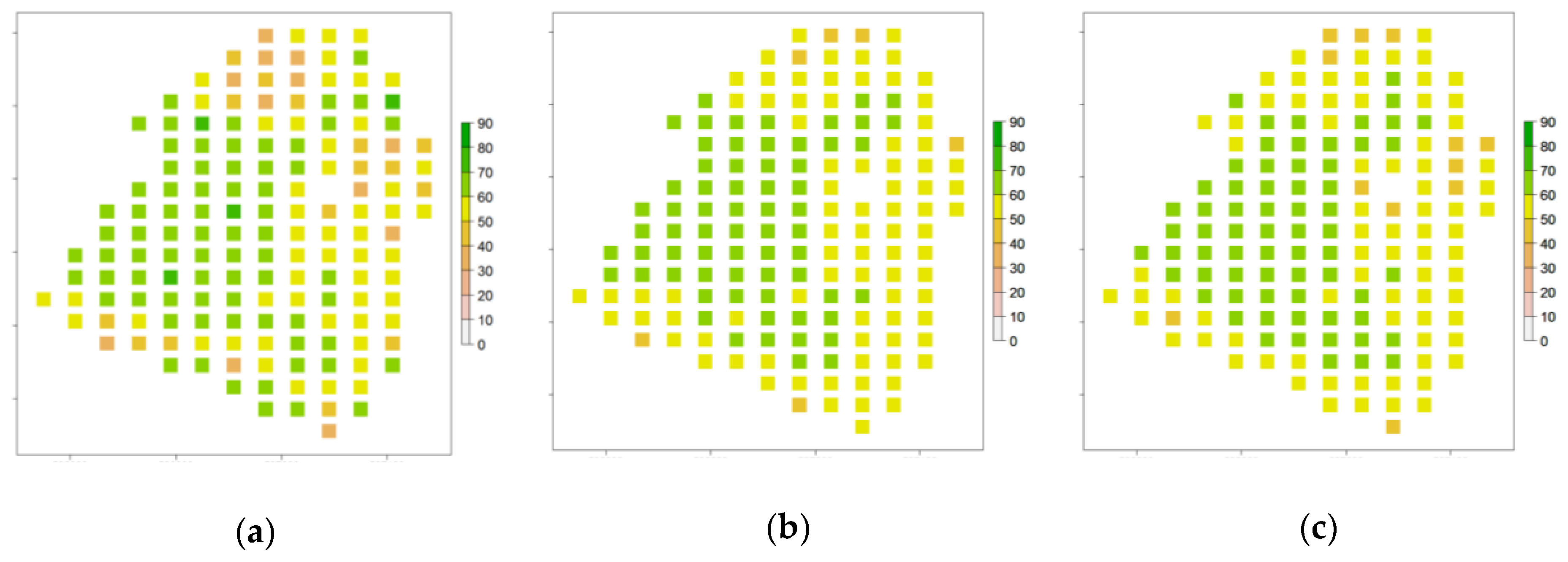
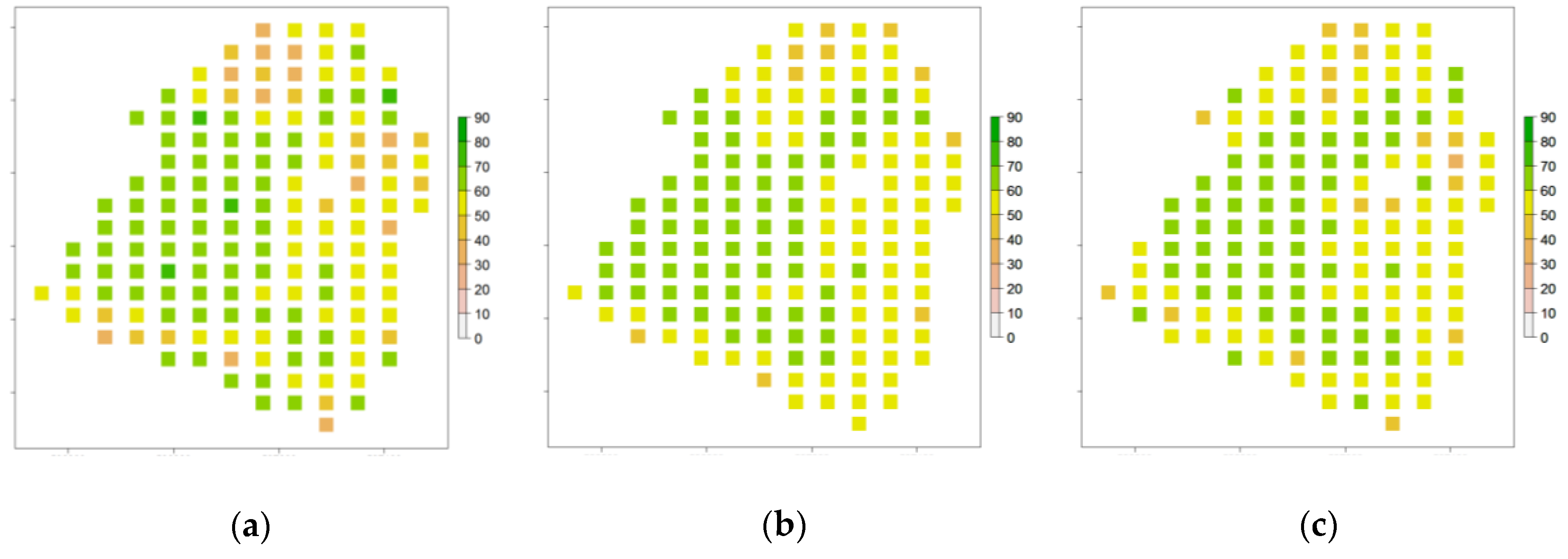
4.2. Analyses of the Yield Maps Collected or Estimated at the Intra-Plot Spatial Scale

4.2.1. Yields Observed during the 2015–2017 Rotation

The analyses of yield maps are focused on one field dedicated to the cultivation of wheat during the agricultural seasons 2015 and 2017 (Figure 5a,b). The values of yields collected on this field are higher in 2015 reaching an average of 61.1 q.ha−1, compared to 57.7 q.ha−1 for the year 2017. The variability of yields is almost similar, as evidenced by the values of the standard deviation of the measured yields (10.0 and 9.4 q.ha−1 for the years 2015 and 2017, respectively). At the intra-plot spatial scale, the patterns showing high and low productive zones are observed at the same or neighboring locations of the plot. Such persistence of the productive areas is characterized by a correlation of 0.69, while the difference between the relative values of yield is mainly inferior to 10% (for more than half of the pixels of the considered plot, Figure 5c). This map allows distinguishing areas with stable behaviors regarding the measured yields (associated with a small relative difference) and areas showing higher variability between the two considered years (with values of relative difference superior to 20% for one-fourth of the pixels of the plot). Finally, the difference in production, which is close to 3.6 q.ha−1 on average, is explained by higher overall production levels within the plot (whether in areas associated with high or low yields).

4.2.2. Yield Estimated Using All the Satellite Acquired Throughout the Agricultural Season

The maps of yields obtained on the monitored field are presented in Figure 6, showing the estimated values based on the NDVI derived from images acquired during the entire agricultural season 2017 (Figure 6a) or based on satellite data combined with the previous yields observed in 2015 (Figure 6b). The two maps of estimated yields exhibit comparable intra-plot spatial patterns, as evidenced by the correlation upper than 0.88 between the two maps. The intra-plot patterns associated with low and high values are well predicted, even if extreme measured values are not well reproduced by the statistical approach. Such an observation is confirmed considering all the pixels of the plot. Indeed, the averages of estimated yields are close (i.e., 58.5 and 58.2 q.ha−1, considering predicted values based on the NDVI or satellite data combined with previous yields) and consistent with the measured yields (57.7 q.ha−1), confirming the ability of the proposed approach to carefully estimate the general behavior. Nevertheless, the observed variability of yields is not totally well reproduced, as evidenced by the higher value of the standard deviation of the measured yields (9.4 q.ha−1) compared to those derived from estimates based on the NDVI (5.1 q.ha−1) or on the combination of satellite images and previous yield map (5.6 q.ha−1).

4.2.3. Yield Estimated Three Months before the Harvest

Figure 7 presents two maps of in-season estimates of wheat yield, obtained using a limited number of satellite images (i.e., acquired between the crop sowing and the month of April). As previously, the estimates are based on satellite data alone or combined with the previously measured yields (Figure 7a,b, respectively). These maps obtained during the elongation of the main stem, on the basis of six satellite images (compared to 12 in the previous section), present estimates close to those observed previously at the end of the agricultural season. The deviations from the plot mean values are thus very small (less than 0.6 q.ha−1, i.e., mean values of 58.5 and 57.6 q.ha−1 for estimates obtained without and with the previous yield map), as is the variability of the estimated yields (5.5 and 6.2 q.ha−1, respectively). This similarity between early and late estimates results in high correlation levels, namely 0.91 and 0.93, although some different spatial patterns may exist. This difference between the "in-season" and "just before harvest" estimates is less than 3 q.ha−1 for more than 80% of the pixels of the plot, whatever the case considered.

5. Discussions

The results presented by [28] provide an interesting comparison with the proposed study, as the estimates are based on a combination of Landsat-8 and Sentinel-2A images. In this study, the estimated winter wheat yields are compared with official statistics at the district level for a study site located in Ukraine, showing a maximal R2 of 0.50 and a relative error of 6.5% for best performance. Furthermore, the magnitude of error obtained on yield estimates is close to the performance presented by [19] (R2 = 0.76 and RMSE = 7.0 q.ha−1), a study based on successive acquired optical and radar images with artificial neural networks for yield retrieval at a field spatial scale.
The performance offered by the proposed statistical approach can also be compared to approaches combining satellite data and crop models through the assimilation scheme. Those more complex methods are characterized by a wide range of performance regarding the estimate of wheat yields (with for instance R2 ranging from 0.50 to 0.91 [16,17,18]) explained by a set of factors such as the complexity of the considered model, the number of parameters, the targeted variable and the method of assimilation. Furthermore, the variability in accuracy in those previous studies is also related to the validation dataset which is often limited to few measurements (due to the difficulty to obtain such information) and acquired at the plot scale. The yields collected at the intra-plot scale by a surveying harvesting machine with GPS system on track mode allows to perform fully independent calibration and validation steps on a large dataset (more than thousands of measurements for each studied year), and to assess the performance of the proposed approach at a spatial scale consistent with the resolution of satellite images.
Agronomic studies have presented interesting results regarding the possibility of obtaining accurate early estimates of wheat yield during the elongation of the main stem [29,30]. Such in-season estimates of crop yields have also been performed by using optical and microwave images [19,31]. In those previous studies, the estimates were performed at the plot spatial scale, showing statistical performance depending on the considered combinations of image frequencies and polarizations. The best statistics for wheat (with an R2 = 0.76 and RMSE = 7.0 q.ha−1) were obtained on about 30 plots surveyed during one agricultural season (using a k-fold cross-validation procedure). The results presented in the proposed study appear consistent with both the agronomics and satellites based on previous studies. Furthermore, the estimates of yields are performed at a finer spatial scale (intra-plot compared to plot scale), testing the robustness of the methodology on four successive years. The forecast of yield has been obtained for the different agricultural seasons and the ability to obtain accurate early estimates of yield regardless of the agricultural season can be addressed by analyzing the differences between early (April) and late (just before harvest) estimates. Over the four years, the difference between the early and late R2 does not exceed 0.1 and that of the RMSE is less than 0.5 q.ha−1 (for estimates based on the use of satellite images and previous or past yield maps). In the proposed study, the gain associated with taking into account images acquired after April and up to harvest therefore appears to be limited.
This result highlights the critical period concerning the acquisition of image dates for the proposed method. A lack of data during this first period of crop development would be detrimental, especially at the end of winter when vegetation growth restarts. Conversely, an absence of images after April would have a limited impact. At this date, the wheat crop is at the stage of stem elongation, and the magnitude of performance only slightly increases thereafter. This limitation of performance is multi-factorial and may be related to agricultural practices. The studied plots are cultivated by different farmers, with, for example, their own sowing practices. It can also be related to the pre-processing of yield data. For each of the plots, 99.7% of the data were kept for this study. More drastic filtering of the data collected by the combine harvester might have allowed obtaining higher levels of performance. Moreover, the limitation of performance may partly be related to the simplicity of the method. A synchronization of crop cycles following the detection of sowing (or early growth stages) may be beneficial to the proposed approach [32]. Finally, events not detected by optical imaging, such as lodging, may be partly responsible for performance limitations. In this case, the detection of impacted areas based on radar images could bring an improvement [6].
Finally, the results presented in this study show the complementarities between two technologies, namely satellite imagery and embedded sensors within agricultural machines, presenting, in particular, a convergence regarding the spatial scale. The ability to reproduce intra-plot spatial patterns of yields based on these optical images provides an interesting perspective in a crop management context. In future studies, this type of satellite-derived information could be integrated into decision-making to modulate crop seeding rates or nutriment inputs before and during the growing season [33,34]. Whether for crop management purposes or to predict yields, future progress will require the identification of areas showing comparable behaviors [35,36]. Understanding the interactions between vegetation, climatic conditions, soil parameters and cultural practices will help to establish the production potential of these entities [37,38]. In this context, the data acquired during successive agricultural seasons provide a valuable basis for analysis. The history of data can thus provide information for monitoring the current season, such as the persistence of spatial patterns regarding yields as in the current study.

6. Conclusions

In this study, a method was implemented to assess the intra-plot yield of wheat at a decametric spatial scale. The description of the seasonality of the vegetation, through the reflectance provided by the Landsat-8 and Sentinel-2 optical images, was the predictive input variable of a statistical algorithm. The image-only approach has benefited from plot tracking history in crop rotations. The proposed approach fits perfectly into the context of precision farming, where access to information on soil and vegetation metrics is increasing, especially harvesting machine collecting yield’s measurements.
The method was evaluated for wheat crops cultivated within the Gers County (southwestern France) during four successive agricultural seasons. From 12 to 14 regular satellite acquisitions were available from the sowing to the harvest of the crop, allowing comparing the yield’s predictive capacities provided by the NDVI or the combined use of six spectral bands. The magnitudes of error on yield estimates appear acceptable, values of RMSE being lower than the observed variability, whatever the considered year (mean standard deviation of 11.8, 9.8, 10.0 and 8.9 q.h−1 for the yields collected in 2014, 2015, 2016 and 2017, respectively). The times series of NDVI combined with the previous or past yield maps provided best yield estimates, the agricultural season 2014 showing the lower level of performances (R2 of 0.44 and a RMSE of 8.13 q.h−1), while the three other years were associated with values of R2 close or upper than 0.60 and RMSE lower than 7 q.h−1.
Moreover, the approach fully exploits the revisiting capabilities of satellite missions, providing regular estimates after each new usable acquisition. The performances obtained during the growing season (i.e., during the elongation of the main stem) are not very far from the best performances observed just before the harvest. Spatial patterns, with either high or low production levels, are clearly reproduced three months before the harvest, opening up prospects for modulated management within the plot.
These promising results should be extended to other crops and to other study sites, taking into account additional information often available in precision farming farms (e.g., information on soil through the measurements of resistivity), and by testing the potential offered by other satellite images (e.g., regular microwave images provided by Sentinel-1).

Author Contributions

Funding acquisition, G.D.; supervision, V.B.; formal analysis, V.B., D.C. and R.F.; writing, R.F. All authors have read and agree to the published version of the manuscript.

Funding

This research received no external funding.

Acknowledgments

The authors wish to thank the Theia land data center for providing the level 2A Landsat-8 and Sentinel-2 satellite images. In addition, the authors wish to thank the agricultural cooperative AGRO D’OC, especially Guigues, Gambini and Hypolite, for their time and precious discussion, and the farmers who helped to collect the ground data.

Conflicts of Interest

The authors declare no conflicts of interest.

References

  1. Food and Agriculture Organization of the United Nations or FAO. Available online: http://faostat.fao.org/ (accessed on 25 February 2019).
  2. Agreste. Available online: http://agreste.agriculture.gouv.fr/ (accessed on 25 February 2019).
  3. Marais Sicre, C.; Fieuzal, R.; Baup, F. Contribution of multispectral (optical and radar) satellite images to the classification of agricultural surfaces. Int. J. Appl. Earth Obs. Geoinf. 2020, 84, 101972. [Google Scholar] [CrossRef]
  4. Fieuzal, R.; Baup, F.; Marais Sicre, C. Monitoring wheat and rapeseed by using synchronous optical and radar satellite data—From temporal signatures to crop parameters estimation. Adv. Remote Sens. 2013, 2, 162–180. [Google Scholar] [CrossRef] [Green Version]
  5. Betbeder, J.; Fieuzal, R.; Philippets, Y.; Ferro-Famil, L.; Baup, F. Contribution of multi-temporal polarimetric SAR data for monitoring winter wheat and rapeseed crops. J. Appl. Remote Sens. 2016, 10, 026020. [Google Scholar] [CrossRef]
  6. Yang, H.; Chen, E.; Li, Z.; Zhao, C.; Yang, G.; Pignatti, S.; Casa, R.; Zhao, L. Wheat lodging monitoring using polarimetric index from RADARSAT-2 data. Int. J. Appl. Earth Obs. Geoinf. 2015, 34, 157–166. [Google Scholar] [CrossRef]
  7. Fieuzal, R.; Duchemin, B.; Jarlan, L.; Zribi, M.; Baup, F.; Merlin, O.; Hagolle, O.; Garatuza-Payan, J. Combined use of optical and radar satellite data for the monitoring of irrigation and soil moisture of wheat crops. Hydrol. Earth Syst. Sci. 2011, 15, 1117–1129. [Google Scholar] [CrossRef] [Green Version]
  8. Becker-Reshef, I.; Vermote, E.; Lindeman, M.; Justice, C. A generalized regression-based model for forecasting winter wheat yields in Kansas and Ukraine using MODIS data. Remote Sens. Environ. 2010, 114, 1312–1323. [Google Scholar] [CrossRef]
  9. Kogan, F.; Kussul, N.; Adamenko, T.; Skakun, S.; Kravchenko, O.; Kryvobok, O.; Shelestov, A.; Kolotii, A.; Kussul, O.; Lavrenyuk, A. Winter wheat yield forecasting in Ukraine based on Earth observation, meteorological data and biophysical models. Int. J. Appl. Earth Obs. Geoinf. 2013, 23, 192–203. [Google Scholar] [CrossRef]
  10. Franch, B.; Vermote, E.F.; Becker-Reshef, I.; Claverie, M.; Huang, J.; Zhang, J.; Justice, C.; Sobrino, J.A. Improving the timeliness of winter wheat production forecast in the United States of America, Ukraine and China using MODIS data and NCAR Growing Degree Day information. Remote Sens. Environ. 2015, 161, 131–148. [Google Scholar] [CrossRef]
  11. Jiang, Z.; Chen, Z.; Chen, J.; Liu, J.; Ren, J.; Li, Z.; Sun, L.; Li, H. Application of crop model data assimilation with a particle filter for estimating regional winter wheat yields. IEEE J. Sel. Top. Appl. Earth Obs. Remote Sens. 2014, 7, 4422–4431. [Google Scholar] [CrossRef]
  12. Jin, X.; Li, Z.; Yang, G.; Yang, H.; Feng, H.; Xu, X.; Wang, J.; Li, X.; Luo, J. Winter wheat yield estimation based on multi-source medium resolution optical and radar imaging data and the AquaCrop model using the particle swarm optimization algorithm. ISPRS J. Photogramm. Remote Sens. 2017, 126, 24–37. [Google Scholar] [CrossRef]
  13. Lai, Y.R.; Pringle, M.J.; Kopittke, P.M.; Menzies, N.W.; Orton, T.G.; Dang, Y.P. An empirical model for prediction of wheat yield, using time-integrated Landsat NDVI. Int. J. Appl. Earth Obs. Geoinf. 2018, 72, 99–108. [Google Scholar] [CrossRef]
  14. Nagy, A.; Fehér, J.; Tamás, J. Wheat and maize yield forecasting for the Tisza river catchment using MODIS NDVI time series and reported crop statistics. Comput. Electron. Agric. 2018, 151, 41–49. [Google Scholar] [CrossRef]
  15. López-Lozano, R.; Duveiller, G.; Seguini, L.; Meroni, M.; García-Condado, S.; Hooker, J.; Leo, O.; Baruth, B. Towards regional grain yield forecasting with 1km-resolution EO biophysical products: Strengths and limitations at pan-European level. Agric. Forest Meteorol. 2015, 206, 12–32. [Google Scholar] [CrossRef]
  16. Dente, L.; Satalino, G.; Mattia, F.; Rinaldi, M. Assimilation of leaf area index derived from ASAR and MERIS data into CERES-wheat model to map wheat yield. Remote Sens. Environ. 2008, 112, 1395–1407. [Google Scholar] [CrossRef]
  17. Rinaldi, M.; Satalino, G.; Mattia, F.; Balenzano, A.; Perego, A.; Acutis, M.; Ruggieri, S. Assimilation of COSMO-SkyMed-derived LAI maps into the AQUATER crop growth simulation model. Capitanata (Southern Italy) case study. Eur. J. Remote Sens. 2013, 46, 891–908. [Google Scholar] [CrossRef] [Green Version]
  18. Duchemin, B.; Fieuzal, R.; Rivera, M.A.; Ezzahar, J.; Jarlan, L.; Rodriguez, J.C.; Hagolle, O.; Watts, C. Impact of sowing date on yield and water-use-efficiency of wheat analyzed through spatial modeling and FORMOSAT-2 images. Remote Sens. 2015, 7, 5951–5979. [Google Scholar] [CrossRef] [Green Version]
  19. Fieuzal, R.; Baup, F. Forecast of wheat yield throughout the agricultural season using optical and radar satellite images. Int. J. Appl. Earth Obs. Geoinf. 2017, 59, 147–156. [Google Scholar] [CrossRef]
  20. Niedbała, G. Simple model based on artificial neural network for early prediction and simulation winter rapeseed yield. J. Integr. Agric. 2019, 18, 54–61. [Google Scholar] [CrossRef] [Green Version]
  21. Kowalik, W.; Dabrowska-Zielinska, K.; Meroni, M.; Raczka, T.U.; de Wit, A. Yield estimation using SPOT-VEGETATION products: A case study of wheat in European countries. Int. J. Appl. Earth Obs. Geoinf. 2014, 32, 228–239. [Google Scholar] [CrossRef]
  22. Wang, L.; Zhou, X.; Zhu, X.; Dong, Z.; Guo, W. Estimation of biomass in wheat using random forest regression algorithm and remote sensing data. Crop J. 2016, 4, 212–219. [Google Scholar] [CrossRef] [Green Version]
  23. Drusch, M.; Del Bello, U.; Carlier, S.; Colin, O.; Fernandez, V.; Gascon, F.; Hoersch, B.; Isola, C.; Laberinti, P.; Martimort, P.; et al. Sentinel-2: ESA’s Optical High-Resolution Mission for GMES Operational Services. Remote Sens. Environ. 2012, 120, 25–36. [Google Scholar] [CrossRef]
  24. Roy, D.; Wulder, M.A.; Loveland, T.; Woodcock, C.E.; Allen, R.; Anderson, M.C.; Helder, D.; Irons, J.; Johnson, D.; Kennedy, R.; et al. Landsat-8: Science and product vision for terrestrial global change research. Remote Sens. Environ. 2014, 145, 154–172. [Google Scholar] [CrossRef] [Green Version]
  25. Hagolle, O.; Huc, M.; Villa Pascual, D.; Dedieu, G. A Multi-Temporal and Multi-Spectral Method to Estimate Aerosol Optical Thickness over Land, for the Atmospheric Correction of FormoSat-2, LandSat, VENμS and Sentinel-2 Images. Remote Sens. 2015, 7, 2668–2691. [Google Scholar] [CrossRef] [Green Version]
  26. Rouse, J.W.; Haas, R.H.; Schell, J.A.; Deering, D.W.; Harlan, J.C. Monitoring the Vernal Advancements and Retrogradation of Natural Vegetation; Technical report No. E74-10676; Texas A&M University: College Station, TX, USA, 1974; pp. 1–137. [Google Scholar]
  27. Breiman, L. Random forests. Mach. Learn. 2001, 45, 5–32. [Google Scholar] [CrossRef] [Green Version]
  28. Skakun, S.; Vermote, E.; Roger, J.-C.; Franch, B. Combined Use of Landsat-8 and Sentinel-2A Images for Winter Crop Mapping and Winter Wheat Yield Assessment at Regional Scale. AIMS Geosci. 2017, 3, 163–186. [Google Scholar] [CrossRef]
  29. Bushong, J.T.; Mullock, J.L.; Miller, E.C.; Raun, W.R.; Klatt, A.R.; Arnall, D.B. Development of an in-season estimate of yield potential utilizing optical crop sensors and soil moisture data for winter wheat. Precis. Agric. 2016, 17, 451–469. [Google Scholar] [CrossRef]
  30. Raun, W.R.; Solie, J.B.; Johnson, G.V.; Stone, M.L.; Lukina, E.V.; Thomason, W.E.; Schepers, J.S. In-season prediction of potential grain yield in winterwheat using canopy reflectance. Agron. J. 2001, 93, 131–138. [Google Scholar] [CrossRef] [Green Version]
  31. Fieuzal, R.; Marais Sicre, C.; Baup, F. Estimation of corn yield using multi-temporal optical and radar satellite data and artificial neural networks. Int. J. Appl. Earth Obs. Geoinf. 2017, 57, 14–23. [Google Scholar] [CrossRef]
  32. Yang, H.; Li, Z.; Chen, E.; Zhao, C.; Yang, G.; Casa, R.; Pignatti, S.; Feng, Q. Temporal polarimetric behavior of oilseed rape (Brassica napus L.) at C-Bandfor early season sowing date monitoring. Remote Sens. 2014, 6, 10375–10394. [Google Scholar] [CrossRef] [Green Version]
  33. Wezel, A.; Casagrande, M.; Celette, F.; Vian, J.F.; Ferrer, A.; Peigné, J. Agroecological practices for sustainable agriculture. A review. Agron. Sustain. Dev. 2014, 34, 1–20. [Google Scholar] [CrossRef] [Green Version]
  34. Godwin, R.J.; Wood, G.A.; Taylor, J.C.; Knight, S.M.; Welsh, J.P. Precision Farming of Cereal Crops: A Review of a Six Year Experiment to develop Management Guidelines. Biosyst. Eng. 2003, 84, 375–391. [Google Scholar] [CrossRef]
  35. Blackmore, S.; Godwin, R.J.; Fountas, S. The Analysis of Spatial and Temporal Trends in Yield Map Data over Six Years. Biosyst. Eng. 2003, 84, 455–466. [Google Scholar] [CrossRef]
  36. Gavioli, A.; de Souza, E.G.; Bazzi, C.L.; Guedes, L.P.C.; Schenatto, K. Optimization of management zone delineation by using spatial principal components. Comput. Electron. Agric. 2016, 127, 302–310. [Google Scholar] [CrossRef]
  37. Usowicz, B.; Lipiec, J. Spatial variability of soil properties and cereal yield in a cultivated field on sandy soil. Soil Tillage Res. 2017, 174, 241–250. [Google Scholar] [CrossRef]
  38. Lipiec, J.; Usowicz, V. Spatial relationships among cereal yields and selected soil physical and chemical properties. Sci. Total Environ. 2018, 33, 1579–1590. [Google Scholar] [CrossRef]
Figure 1. Overview of the wheat yield measurements collected at the intra-plot scale during the agricultural seasons 2014–2016 (a) and 2015–2017 (b). The mean and standard deviation values are presented together with correlation between “pair years”.
Agronomy 10 00327 g001
Figure 2. Statistical performance (coefficients of determination and root mean square errors, bars and dots, respectively) associated with the estimation of the wheat yields (considering multi-temporal Normalized Difference Vegetation Index (NDVI) as input variable) as a function of the ratios of training and validation data, for the years 2014 (a), 2015 (b), 2016 (c) and 2017 (d).
Agronomy 10 00327 g002
Figure 3. Statistical performance (coefficients of determination and root mean square errors, in black and gray, respectively) associated with the estimation of the intra-plot wheat yields, for the years 2014, 2015, 2016 and 2017.
Agronomy 10 00327 g003
Figure 4. Temporal evolution of the statistical performances (coefficients of determination and root mean square errors, crosses and dots, respectively) associated to the wheat yield forecast using NDVI (left) or the combination of six reflectance (right), for the years 2014 (a,b), 2015 (c,d), 2016 (e,f) and 2017 (g,h).
Agronomy 10 00327 g004aAgronomy 10 00327 g004b
Figure 5. Maps of wheat yield (expressed in q.ha−1) collected on a plot dedicated to the cultivation of wheat in 2015 (a) and in 2017 (b), together with the differences between the relative values of yields (expressed in percent) (c).
Agronomy 10 00327 g005
Figure 6. Maps of yield (expressed in q.ha−1) collected in 2017 (a), and estimated using multi-temporal NDVI derived from images acquired throughout the agricultural season (b), or the combination of satellite data and previous observed yields (collected during the agricultural season 2015) (c) on a plot dedicated to the cultivation of wheat.
Agronomy 10 00327 g006
Figure 7. Maps of yield (expressed in q.ha−1) collected in 2017 (a), and estimated using multi-temporal NDVI derived from images acquired from the sowing to the month of April (04/06/2017) (b) or the combination of satellite data and previous observed yields (collected during the agricultural season 2015) (c) on a plot dedicated to the cultivation of wheat.
Agronomy 10 00327 g007
Table 1. Characteristics of the satellite remote sensing data.
Season 2014Season 2015Season 2016Season 2017
SatelliteDateSatelliteDateSatelliteDateSatelliteDate
Landsat-823 October 2013Landsat-826 October 2014Landsat-830 November 2015Sentinel-217 November 2016
Landsat-810 December 2013Landsat-820 November 2014Sentinel-23 December 2015Sentinel-217 December 2016
Landsat-812 February 2014Landsat-822 December 2014Sentinel-223 December 2015Sentinel-215 February 2017
Landsat-89 March 2014Landsat-829 December 2014Landsat-825 December 2015Sentinel-225 February 2017
Landsat-816 March 2014Landsat-814 January 2015Landsat-817 January 2016Sentinel-217 March 2017
Landsat-81 April 2014Landsat-88 February 2015Sentinel-222 March 2016Sentinel-26 April 2017
Landsat-810 April 2014Landsat-813 April 2015Landsat-830 March 2016Sentinel-26 May 2017
Landsat-817 April 2014Landsat-820 April 2015Sentinel-211 April 2016Sentinel-216May 2017
Landsat-819 May 2014Landsat-829 April 2015Landsat-815 April 2016Sentinel-226 May 2017
Landsat-813 Jun 2014Landsat-86 May 2015Sentinel-221 May 2016Sentinel-25 Jun 2017
Landsat-820 Jun 2014Landsat-831 May 2015Landsat-89 Jun 2016Sentinel-225 Jun 2017
Landsat-822 Jul 2014Landsat-87 Jun 2015Sentinel-220 Jun 2016Sentinel-25 Jul 2017
--Landsat-823 Jun 2015Landsat-84 Jul 2016--
--Landsat-89 Jul 2015Sentinel-210 Jul 2016--

