Article

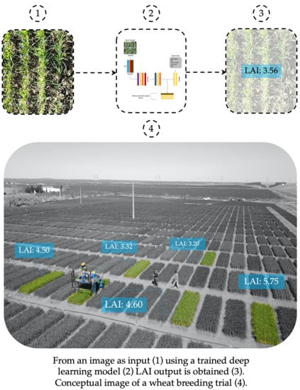
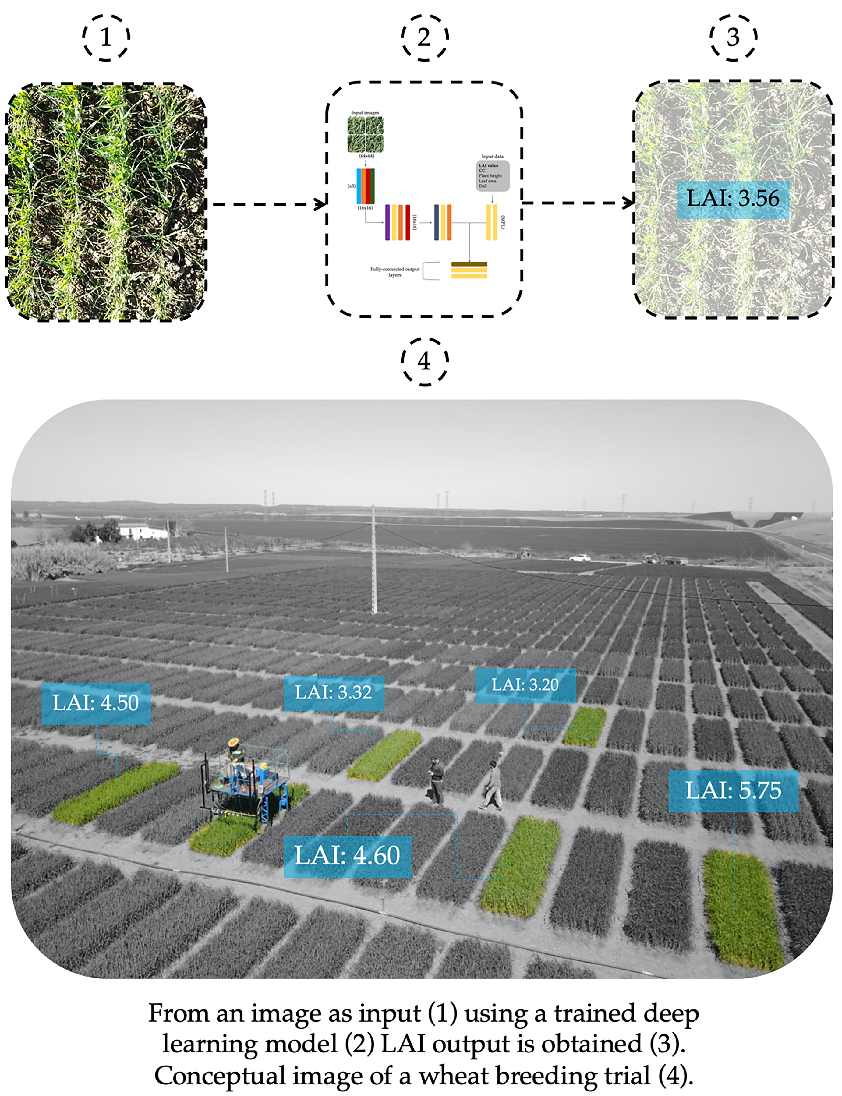
A Mixed Data-Based Deep Neural Network to Estimate Leaf Area Index in Wheat Breeding Trials

by
Orly Enrique Apolo-Apolo
,
Manuel Pérez-Ruiz
,
Jorge Martínez-Guanter
and
Gregorio Egea
*
Area of Agroforestry Engineering, Technical School of Agricultural Engineering (ETSIA), Universidad de Sevilla. Ctra. Utrera km 1, 41013 Sevilla, Spain
*
Author to whom correspondence should be addressed.
Agronomy 2020, 10(2), 175; https://doi.org/10.3390/agronomy10020175
Submission received: 27 November 2019 / Revised: 15 January 2020 / Accepted: 16 January 2020 / Published: 26 January 2020
(This article belongs to the Special Issue Selected Papers from 10th Iberian Agroengineering Congress)

Abstract

:
Remote and non-destructive estimation of leaf area index (LAI) has been a challenge in the last few decades as the direct and indirect methods available are laborious and time-consuming. The recent emergence of high-throughput plant phenotyping platforms has increased the need to develop new phenotyping tools for better decision-making by breeders. In this paper, a novel model based on artificial intelligence algorithms and nadir-view red green blue (RGB) images taken from a terrestrial high throughput phenotyping platform is presented. The model mixes numerical data collected in a wheat breeding field and visual features extracted from the images to make rapid and accurate LAI estimations. Model-based LAI estimations were validated against LAI measurements determined non-destructively using an allometric relationship obtained in this study. The model performance was also compared with LAI estimates obtained by other classical indirect methods based on bottom-up hemispherical images and gaps fraction theory. Model-based LAI estimations were highly correlated with ground-truth LAI. The model performance was slightly better than that of the hemispherical image-based method, which tended to underestimate LAI. These results show the great potential of the developed model for near real-time LAI estimation, which can be further improved in the future by increasing the dataset used to train the model.

Graphical Abstract

1. Introduction

The world’s population is expected to increase to about 9 billion people by 2050 [1]. In this context, food production will need to increase by 70% despite the limited availability of arable lands, the increasing need for fresh water and the impact of climate change [2]. This increase will have to occur in all crops, but especially in those staple crops such as wheat, which provide about 20% of the daily caloric intake for a human being [3]. Thus, the demand for wheat is expected to increase by around 60% in the next few decades, but the potential yield is expected to decrease by 20% due to the climate change [4]. Added to this perspective is the fact that breeders have only achieved an increase in wheat yield of less than 1% per year while forecasts demand an increase of around 2% to meet the growing global food demand [5,6].
Conventional breeding cycle takes years (even decades) to develop and evaluate new breeding lines [7]. The main reason for this is that new cultivars need to be tested at multiple locations over several years to make sure the target environments are covered [8]. A large part of the work done by breeders consists of evaluating cultivars in the field by taking data manually to support decision-making [9]. This process is costly and time-consuming, since measurements are carried out over thousands of small plots which require time and specialized technicians [2]. To bridge this gap, breeders demand solutions which will allow them to evaluate cultivars in the field faster and cheaper [10]. In this context, high-throughput plant phenotyping using aerial and terrestrial platforms has emerged as a promising tool [11,12]. This kind of platform allows accurate remote sensing of crop responses to abiotic and biotic stresses [13,14]. Moreover, automated phenotyping platforms usually measures in a non-destructive way, allowing breeders to evaluate the same plant multiple times throughout the season [15].
Among the large number of phenotypes of interest to be monitored in breeding programs, biophysical crop variables are considered especially important [16]. These variables provide information about a crop’s health status since they are affected by both physical and biological crop traits that are in turn influenced by biotic and abiotic stresses [17]. The leaf area index (LAI), biomass, plant height, the fraction of vegetation cover and the fraction of absorbed photosynthetically active radiation (FPAR) are some of these variables of interest [18]. The LAI is defined as the leaf area of the canopy per unit area projected on the soil [19,20], or as the photosynthetically active leaf area per unit soil area [21,22]. Its value is extremely descriptive as an indicator of the ability of the canopy to intercept incoming photosynthetically active radiation (PAR) [23]. Moreover, due to carbon being fixed by the interception of radiation and then converted into chemical energy, this index can be used to estimate the crop final yield [24]. The LAI is also affected by abiotic stresses such as drought and is a good tool for evaluating the growth and development of crops in breeding programs [25].
Methods for LAI estimation are grouped in direct and indirect methods, and have been widely assessed and reviewed in the literature [19,26]. Direct methods are the most accurate and helpful for validating indirect measurements, but they are extremely time-consuming and prohibitively expensive when applied to large crop areas [20]. Moreover, their application in breeding programs would be of little use since they are often destructive and the sampled area within the small plots could be non-representative and lead to biased results [4,21]. Alternatively, in recent years, indirect methods based on bottom-up hemispherical photography, FPAR-inversion, spectral reflectance measurements and 3D point-clouds analysis have been developed [19,22,27,28]. The essence of the indirect methods is related to how light interacts with the canopy as measured in three ways: transmission, absorptance, and reflectance [29]. Among all the indirect methods available for estimating LAI, the technique that uses hemispherical images taken with a fisheye-type lens is the most used due to its robustness [30,31]. This method is based on the estimated position, size, density, and distribution of canopy gaps, which characterize the canopy geometry through which the intercepted solar radiation is measured [32]. The gap fraction is calculated using thresholding in order to distinguish pixels that are occupied by leaves from pixels that are occupied by the sky or ground [33]. Hence, images under uniformly diffuse light conditions to avoid sun spots in the background are required [34]. In addition to light conditions, the resolution, especially for small leaves and tall canopies, is another potential limitation [19].
Despite indirect methods being quite accurate, the repeatability in image capture still requires time-consuming post-processing [19,25]. The development of deep neural networks, also known as deep learning (DL) techniques, a subset of machine learning (ML) and, specifically, convolutional networks (CNN or ConvNet), has emerged as a powerful less time-consuming and less costly alternative to estimate LAI and many others basic plant phenotyping tasks [35,36]. For example, Lue et al. [37] developed an in-field automatic wheat disease diagnosis system based on a weekly supervised deep learning framework using red green blue (RGB) images. A model to detect and characterize wheat spikes from wheat images as the input was designed by Hasan et al. [38]. Ma et al. [39] proposed a deep learning model to estimate the ground biomass of winter wheat from images captured under field conditions. In terms of LAI estimation, Durbha et al. [40] suggested a method based on support vector machine regression (SVR) using multiangle imaging spectroradiometry of wheat. An approach that includes images from Sentinel 2A as input and manual measurements of LAI using an LAI-2000 Plant Canopy Analyzer (Li-Cor, Inc., Lincoln, NE, USA) was proposed by Jin et al. [41] for LAI estimation in maize microplots. Houborg and McCabe [42] applied a hybrid training approach on the basis of two common decision tree regression algorithms (cubist and random forest models). These tools have demonstrated high accuracy, but low scalability for terrestrial use in a high-throughput phenotyping platform (HTPP) due to the required deployment of proximal sensors with high-resolution imaging technologies suitable to plot sizes [43]. Nevertheless, according to Tsaftaris et al. [44], many of the tools based on images developed for plant phenotyping require prior processing, and this has several drawbacks which add a new bottleneck to the breeding process. On the other hand, some researchers suggest that development in the leaf area carried out during the middle and late crop growth stages do not produce any changes in the crop canopy cover (CC) [45]. Hence, LAI values could still be increasing even when the crop canopy already covers approximately 70%–80% of the ground area. This means that LAI estimation using only data from image segmentation can be improved by adding other parameters that affects the growth and development of plants, as recently shown by Longson and Cambardella [46] who developed a statistical model to determine LAI from ground cover and plant height measurements.
Taking all this into consideration, the aim of this paper was to investigate the suitability of using field-based nadir-view RGB images taken from a high-throughput phenotyping platform to obtain high-accuracy LAI estimates and provide reliable data for wheat breeding programs. The specific objectives, given this approach, were the following: (i) to develop an allometric relationship for non-destructive yet direct estimates of LAI to be used as ground truth; (ii) to build a DL model that combines images and numerical features of the crop for accurate LAI estimations; and (iii) to compare the results obtained by the DL model approach with those obtained by the direct method using the allometric relationship and a commonly used indirect method based on bottom-up hemispherical images taken underneath the vegetation.

2. Materials and Methods

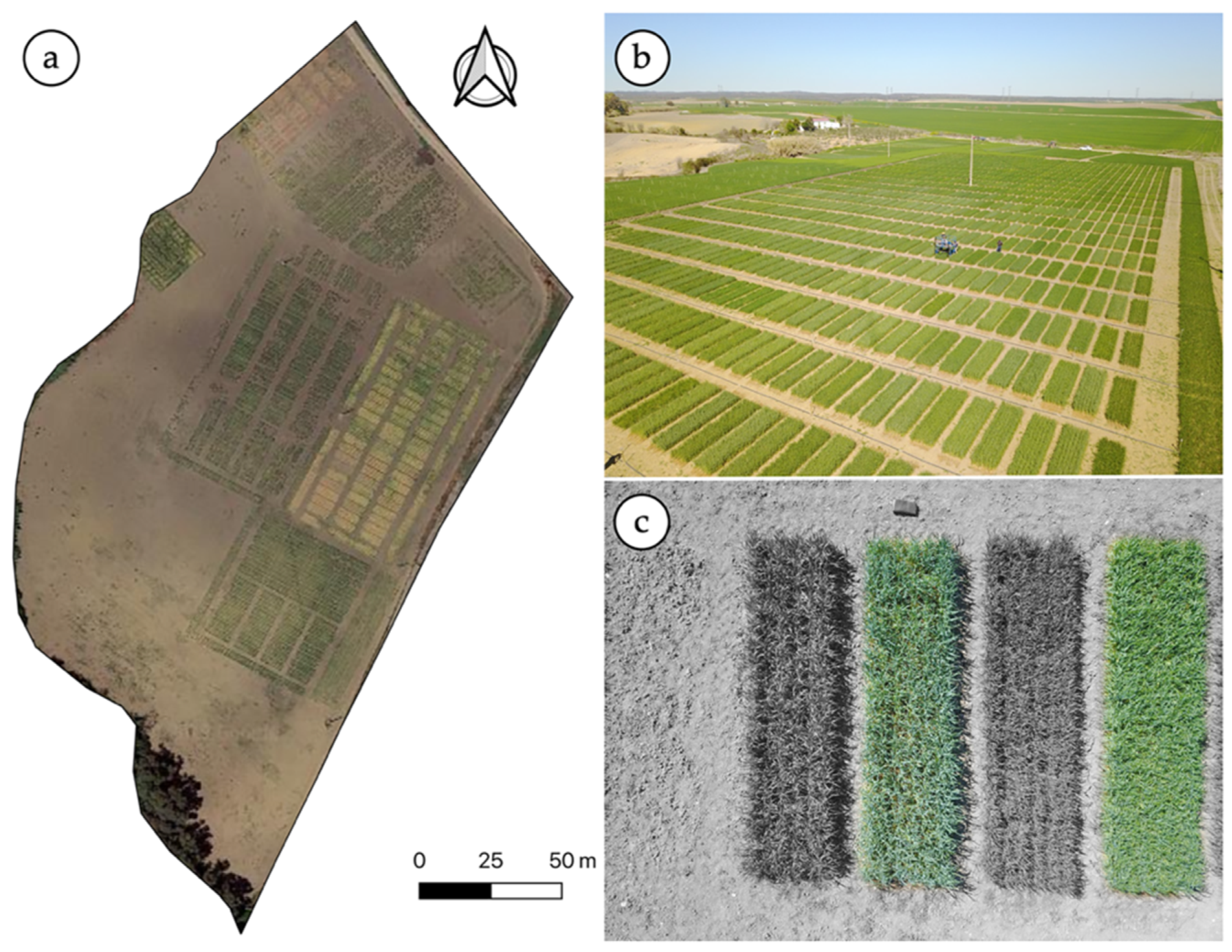
2.1. Description of the Experimental Site

The experiment was performed at an experimental field located in Escacena del Campo, Huelva, Spain (latitude: 37.4525 N; longitude: 6.36194 W) that belongs to the wheat breeding company (Agrovegetal S.A., Seville, Spain). The trial was conducted during two experimental seasons (2017–18 and 2018–19) under rainfed conditions. In the first season, wheat was sown on 25 November 2017 and harvested on 15 June 2018. In the second season, the wheat was sown on 6 December 2018 and harvested 183 days after sowing (DaS), that is, on 7 June 2019. A total of 10 cultivars and three replicates per cultivar were selected from a trial with 25 cultivars and three replicates per cultivar in a randomized block design (Figure 1). The cultivars investigated were the following: Antequera, Conil, Galera, Gazul, Marchena, Montalbán, THA 3753, THA 3829, Tujena, and Valbona. The initial plot dimensions were 6.50 m long by 1.20 m wide according to the working width of the seed sowing machine. Thirty DaS, the plots were resized along their longitudinal dimension with an herbicide application, setting as final dimensions for each plot 6 × 1.20 m. The weather conditions for both growing seasons were dry, as is usual in the region. During the second season, a single irrigation event of 80 mm was applied on 6 March due to an extended spring drought.

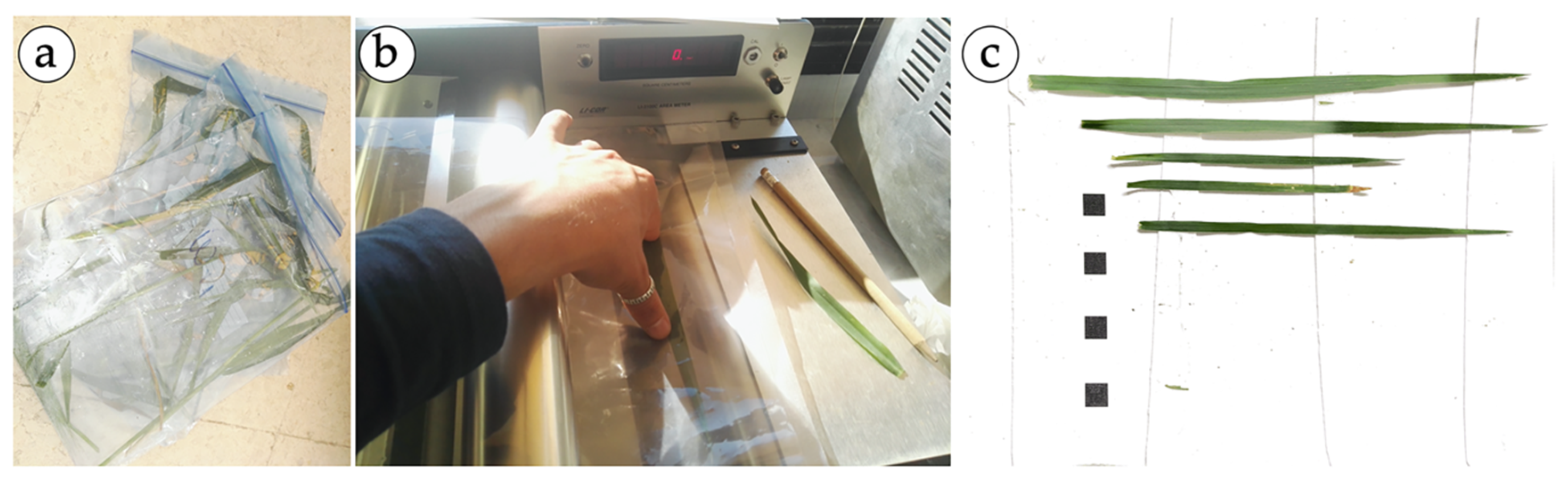
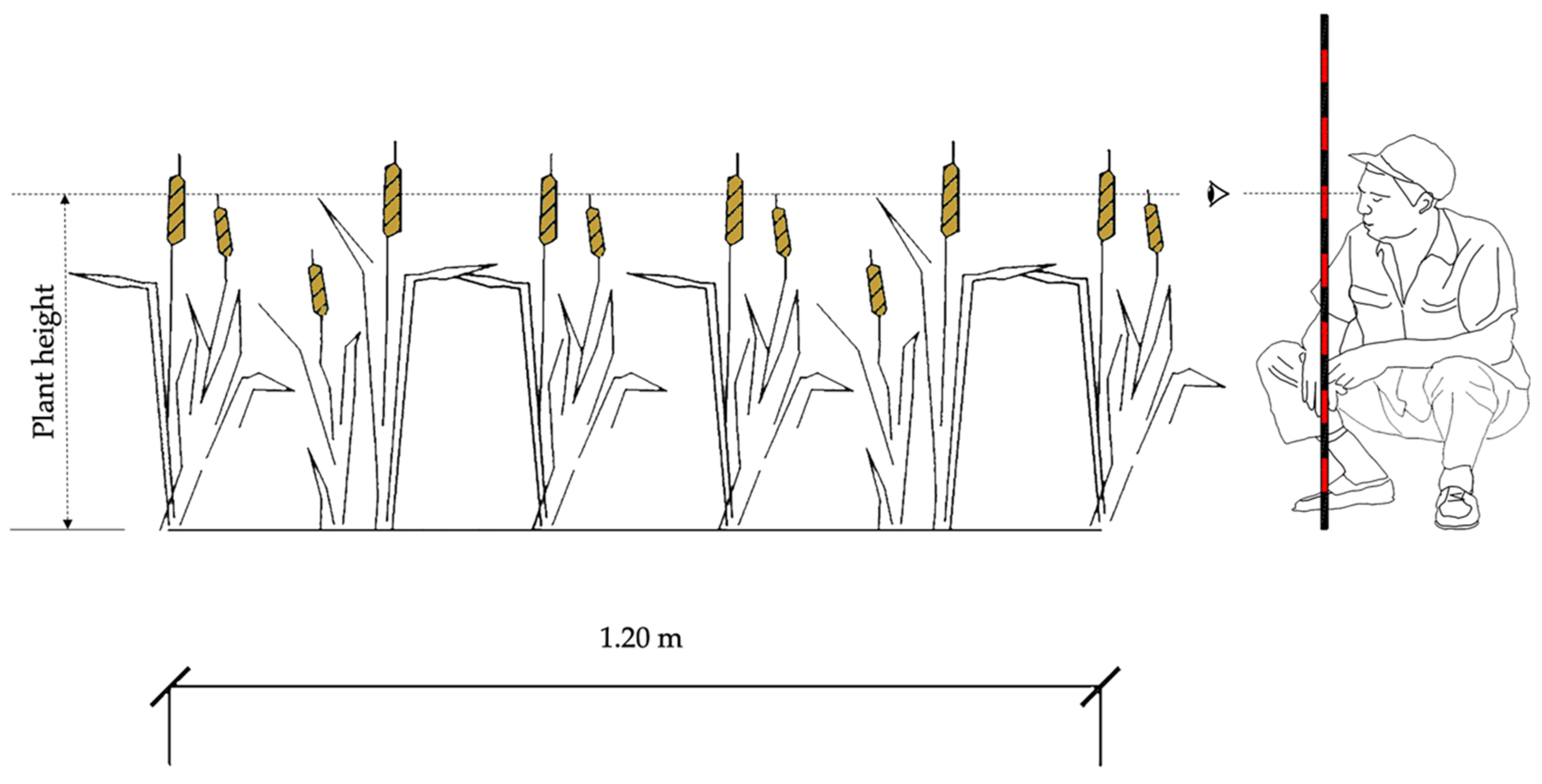
2.2. Allometric Relationship and Direct Estimates of Leaf Area Index (LAI)

Destructive measurements are the only way to validate LAI estimations [19]. So, during both trial seasons, three plants per plot were taken from the zone which was later resized with an herbicide application. Consequently, the conditions of the experimental unit were not affected. Then, the leaves were stored in cooler containers and immediately taken to the laboratory for analyses (Figure 2a). For each leaf, the main linear dimensions, length (L) and maximum width (W), were measured. Then, during the first season (2018), the area of the leaves was measured using a leaf area meter (LI-COR 3100; LI-COR Biotechnology, Lincoln, NE, USA). In the second season (2019), the leaves were placed on a sheet of paper with a square of known dimensions (1 cm2) in the background, as shown in Figure 2c. The ImageJ® software was used to measure the leaf area and its dimensions, as proposed by Ahmad et al. [47]. With all this information, an allometric relationship to derive the leaf area of individual leaves from L and W measurements was developed.
With the purpose of validating the LAI estimated with the DL model through the growing season, three randomly selected representative plants per plot were marked. On the same days that the digital photographs were taken (Table 1), the linear dimensions (L, W) of all plant leaves and the plant height were measured for each selected plant using a flexible tape graduated in millimeters, as shown in Figure 3. The measured dimensions were used to calculate the leaf area of each individual leaf using the abovementioned allometric relationship. The plant leaf area was then calculated as the sum of all the unitary leaf areas. The LAI for all plots was obtained according to the following expression:
L A I = P L A   ( m 2 ) P S   ( m 2 )
where PLA is the plant leaf area and PS the plant spacing, estimated as the inverse of plant density.

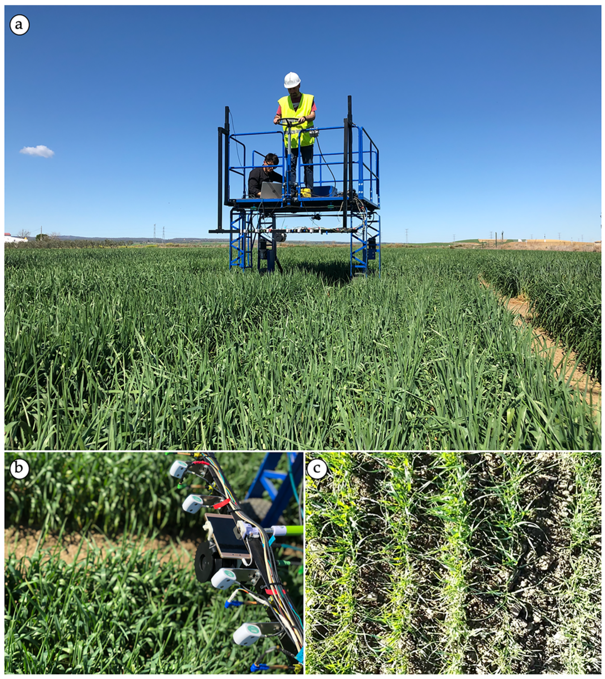
2.3. Image Acqusition and Processing for Deep Learning (DL) Model

Most methods reviewed in the literature use single high-resolution images taken at different locations inside the crop field [29]. This provides an average LAI value of the entire crop area, which might prove to be sufficient for a commercial wheat field. However, this may be not enough for the small plots used in breeding programs, since large within-plot differences in crop parameters, such as plant height, among others, are often observed [2,8]. On the other hand, it is known that a video is composed of several frames (images) where each image is taken automatically, one after the other, producing the impression of a moving image [48]. The number of frames per second (fps) that a camera is able to obtain depends on the technical features of the sensor in question. In order to overcome the existing within-plot crop variability, breeders use replicates to increase confidence in their results [12,14]. In this study, a smartphone model Huawei P8 was located at the front of an HTPP platform (Figure 4a) at a height of 0.50 m over the average wheat canopy height. The device was used to take nadir-view images and to record a video along the entire plot (Figure 4b). The smartphone was driven alongside each plot at a speed of 0.27 ± 0.09 m s−1. Each digital video was recorded with an average recording duration of 25–30 s. The smartphone used in this experiment was able to acquire 30 fps. Bearing this in mind, a Python script was developed to obtain all frames from each one of the videos recorded. An average of 500 frames (Figure 4c) per video was obtained using this code. However, only 20 images per plot were selected to avoid including images from the perimeter of the plot (border effect). Moreover, a method suggested by Rosebrock [49] for image segmentation, where color boundaries (lower and upper) in the RGB color space are established, was adopted to extract the CC value for each image. More details are provided in the Supplementary Material (S1). This information was used as an input in the DL model, which will be explained in Section 2.5.

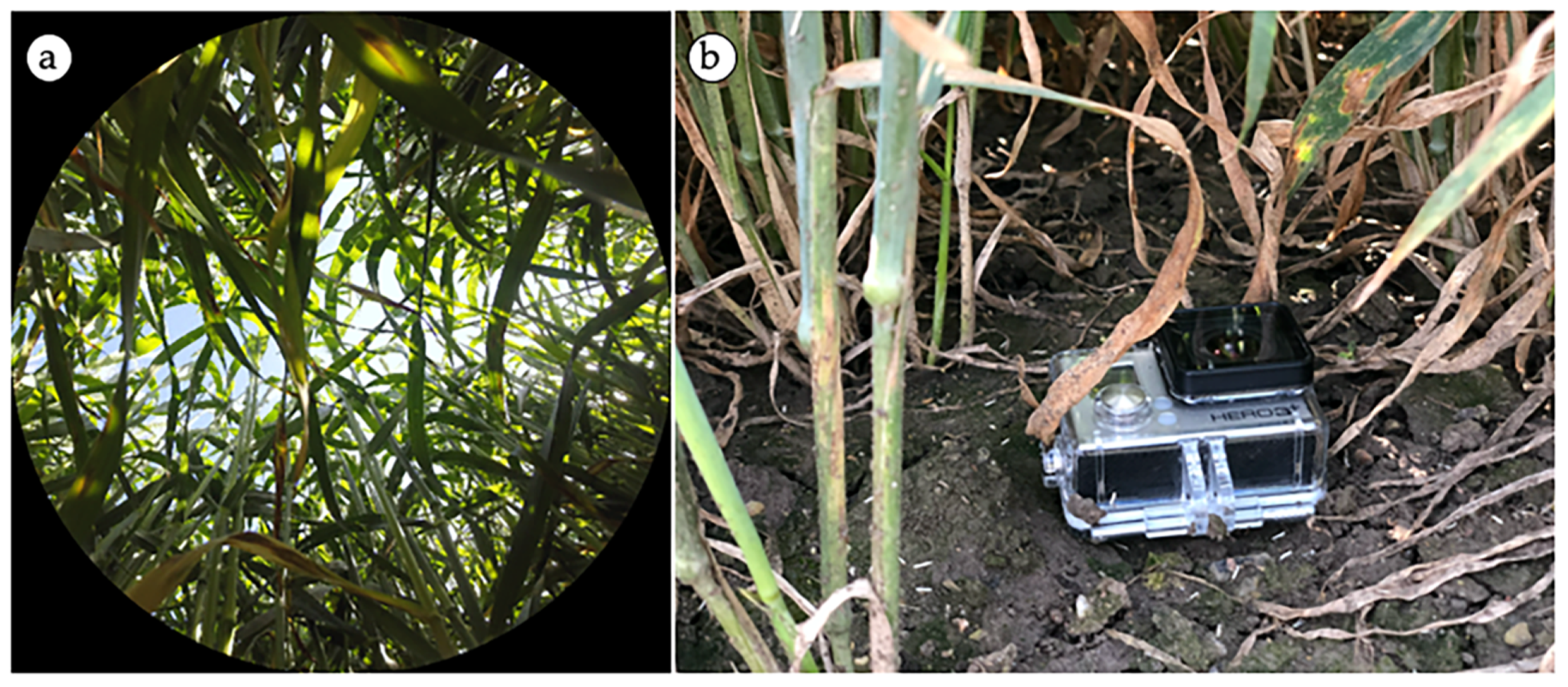
2.4. Hemispherical Images Acquisition and Processing

According to Jonckheere et al. [19], bottom-up hemispherical images can provide precise indirect estimates of LAI. This kind of image is captured using a fisheye-type lens that allows taking pictures with a field of view (FOV) of around 180 degrees. A GoPro camera (Hero3+, GoPro, San Mateo, CA, USA) was used in this work to take the bottom-up hemispherical images. To accomplish this, the camera was equipped with a fisheye lens with an FOV close to 170 degrees [50]. To obtain the bottom-up hemispherical images (Figure 5a) the camera was placed on the ground underneath the plants and located in the center of each plot with the interval timer shooting mode on (Figure 5b).
Both the videos and images were acquired according to the specifications of each device, shown in Table 2. The bottom-up hemispherical images were analyzed using the Can-Eye software (see Supplementary Material (S2) for further details), developed by the French National Institute of Agronomical Research (INRA), as suggested by Demarez et al. [30]. This image-processing method provides LAI and CC estimations, along with others crop parameters related to canopy architectural traits. This is a laborious and time-consuming task, since a manual segmentation process to differentiate between sky (background) and canopy pixels is required.

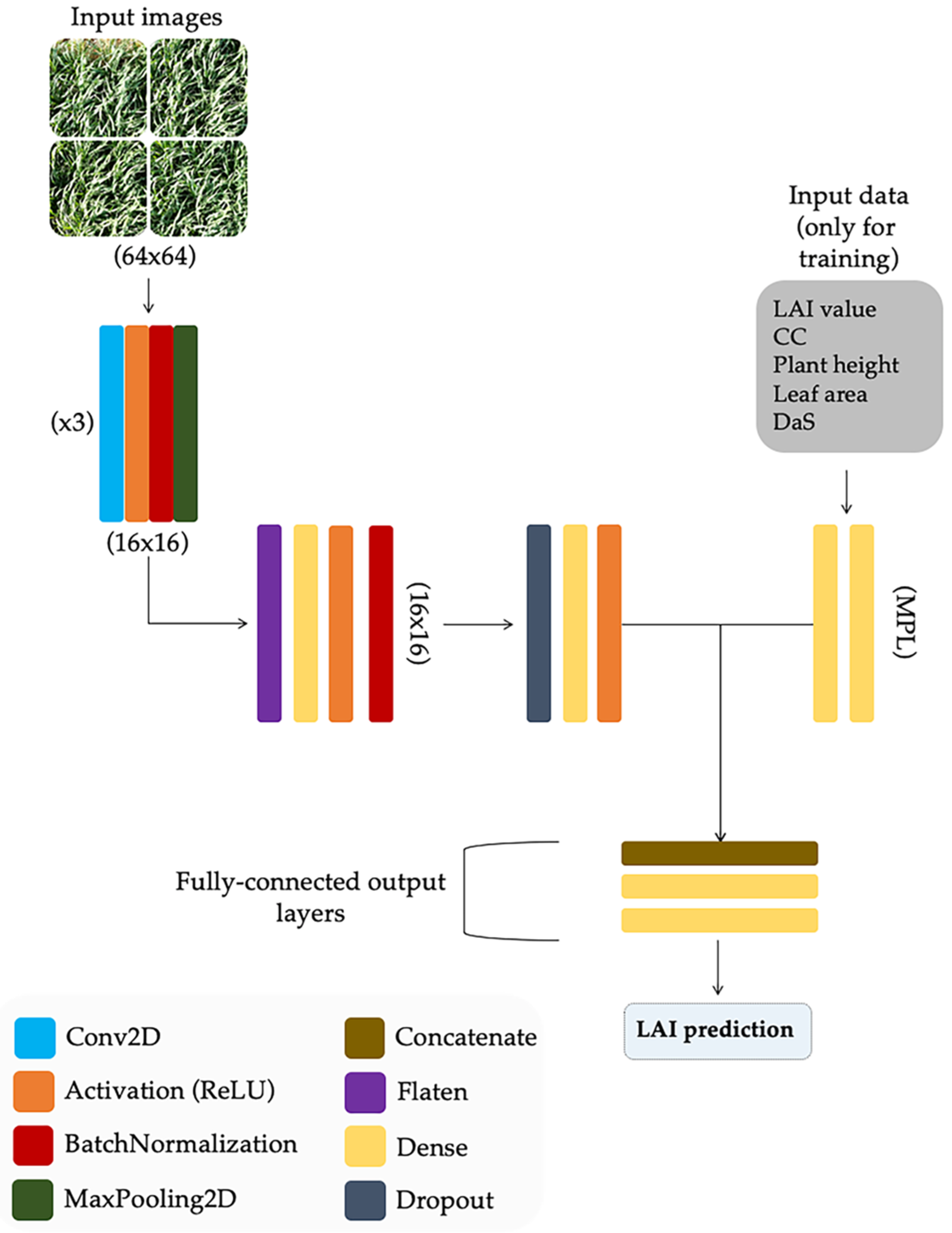
2.5. Deep-Learning Model Description

Most studies carried out on LAI estimation have focused on using only visual features from the images. These methodologies are suitable in some controlled-conditions scenarios but they are time-consuming, of doubtful accuracy and labor-intensive due to the required image pre-processing. To overcome these limitations, a new approach based on deep-learning modeling is proposed, mixing visual features from images and plant architectural parameters measured at ground level to train the model.
According to Gulli and Pal [51], mixed-data neural networks are more complicated in structure but they are more accurate at making predictions than those using only one type of data in the training process. Consequently, the Keras functional API (application programming interface) [52] was used in this study to define the model. This API provides the flexibility needed to define a model that takes different forms of data as inputs and subsequently combines them [51,53]. In this way, a multi-input network with two branches for both images and data was built, as depicted in Figure 6. The first branch consisted of a multilayer perceptron (MLP) with two layers: a fully connected (Dense) input layer and a fully connected hidden layer, both with ReLU (Rectified Linear Unit) activation. This structure was designed to handle numerical inputs (i.e., plant height, CC, DaS, etc.). The other branch was a CNN which used RGB color images as input. This network was composed of three convolution layers placed in a sequential manner with a 2D convolutional neural network followed by batch normalization, ReLU activation, and max-pooling. At the end of these three convolution layers, the next layer was flattened, and then a fully connected (FC) layer with batch normalization, density, and a dropout rate of 50% was added. The max-pooling, dropout, and dense layers were used to reduce the parameters and boost the training. Subsequently, another FC layer was applied to match the nodes coming out of the multi-layer perceptron. This latter step is not a requirement, but it was added to support and balance the branches [54]. Finally, the outputs of both branches were concatenated together to be used as input in the final set of layers of the network. This part of the model had an FC layer with two dense layers, where the final one was used as a regression and its output was the LAI estimation value.
In order to train the model according to the neural network structure, a dataset with the data collected from six out of seven sampling dates (Table 1) was built and structured as follows: each wheat plot was represented by groups of 5 images tiled into one montage of 4 images (20 images for each wheat plot in total). Each montage was associated with a numerical value of the CC, plant height, average leaf area of an individual wheat leaf per plot, DaS, and LAI. A total of 3600 images were used in the training process. Images from DaS 58 were excluded for model training and used for validation purposes. In order to evaluate the effect on model performance of adding crop traits as input parameters of the DL model during the training process, the model was trained in four stages: (i) the model was trained using only RGB images, CC and LAI values, (ii) the plant height was added as an additional parameter together with those previously used, (iii) the average leaf area of an individual wheat leaf per plot was added and (iv) the DaS was included as a final parameter to be used as input for model training. The number of nodes in the MPL was updated according to the inputs in each of the stages. The dataset was split into three subsets: 70% for training, 15% for validation, and 15% for testing, as suggested by Rosebrock [54] for this kind of models. The whole model was compiled using the mean absolute percentage error (MAPE) as a loss function and the Adam’s optimization algorithm [55] as an optimizer with a learning rate of 0.001 and a decay factor of 0.001/200. Finally, when fitting the model, all the weights were tuned by backpropagation; the number of epochs used and the batch sizes were 200 and 8, respectively.
Due to CNN’s high requirements in terms of hardware and graphics processing unit (GPU) resources, Google Colaboratory (also known as Colab) offered by Google was used to implement and train the model. Colab, a cloud service based on Jupyter Notebooks, provides a free single 12 GB NVIDIA Tesla K80 GPU that can be used for up to 12 h continuously. For the local computing processes, a MacBook Pro laptop (MacOs High Sierra 10.13.4) with a 2.5 GHz Intel Core i7 processor, 16 GB of RAM, and AMD Radeon R9 M370X 2048 MB/Intel Iris Pro 1536 MB graphics was used. The Open-Source Computer Vision (OpenCV) library [56], which includes several hundred computer vision algorithms, was used to process images [54].

2.6. Statistical Analysis

Linear regressions were used to compare LAI values estimated using direct and indirect methods. The analysis was performed using RStudio® [57]. The mean absolute error (MAE, Equation (1)) and the Root-Mean-Square Error (RMSE, Equation (2)) were used.
M A E = 1 n t = 1 n | A t F t |
R M S E = t = 1 n ( A t F t ) 2 n
Here, n refers to the number of compared values, At is the actual observed value, Ft is the forecast value and A ¯ t is the actual observed mean value. The RMSE and MAE represent the average differences between the model Ft and the At values. However, it is a normalized statistic that determines the relative magnitude of the residual variance (“noise”) compared to the measured data variance (“data or information”). It is important to include these absolute error measures in model evaluation because they provide an estimate of model error in the units of the variable. The MAE provides a more robust measure of average model error than the RMSE since it is not influenced by extreme outliers [58].
Finally, analysis of variance (ANOVA) was used to determine the significant differences (p < 0.05) among cultivars in terms of LAI values obtained. Means separation was performed using Duncan’s multiple range test.

3. Results and Discussion

3.1. Allometric Relationships for Direct LAI Estimation

Obtaining an allometric relationship to estimate the leaf area of individual wheat leaves in a non-destructive way is of great interest for the validation of other non-destructive methods in trials where the plant material cannot be sampled. This occurs in crop breeding trials where variation in the number of plants per subplot would alter the productivity results of the cultivars. In this paper, two empirical relationships have been derived (Table 3), one for each growth period. Both relationships were based on a first-degree equation, y = ax + b, where the independent variable was calculated as the product of W and L, and a and b are, respectively, the slope and intercept of the linear relationship. The derived relationships explained 91% and 94% of the observed variability in the leaf area of individual leaves in the first and second season, respectively. Slope values of 0.75 cm2 cm−2 and 0.78 cm2 cm−2 were obtained for the first and second season, respectively. Intercept values of −0.9 cm2 and 0.5 cm2 were also observed for the respective two seasons. Similar results were reported by Chanda and Singh [59]. However, the number of observations in their study was slightly lower. Other research carried out by Calderini et al. [60] reported a slope value of 0.83. The authors also made measurements during two seasons, although they sampled five plants per plot, likely giving a most robust predictor. Bryson et al. [61] also obtained a slope value of 0.83 with a coefficient of determination of 0.95 in a field trial with 20 winter wheat varieties. In this study we decided to use a single relationship derived with the pooled data of both experimental seasons, as suggested by Chanda and Singh [59].

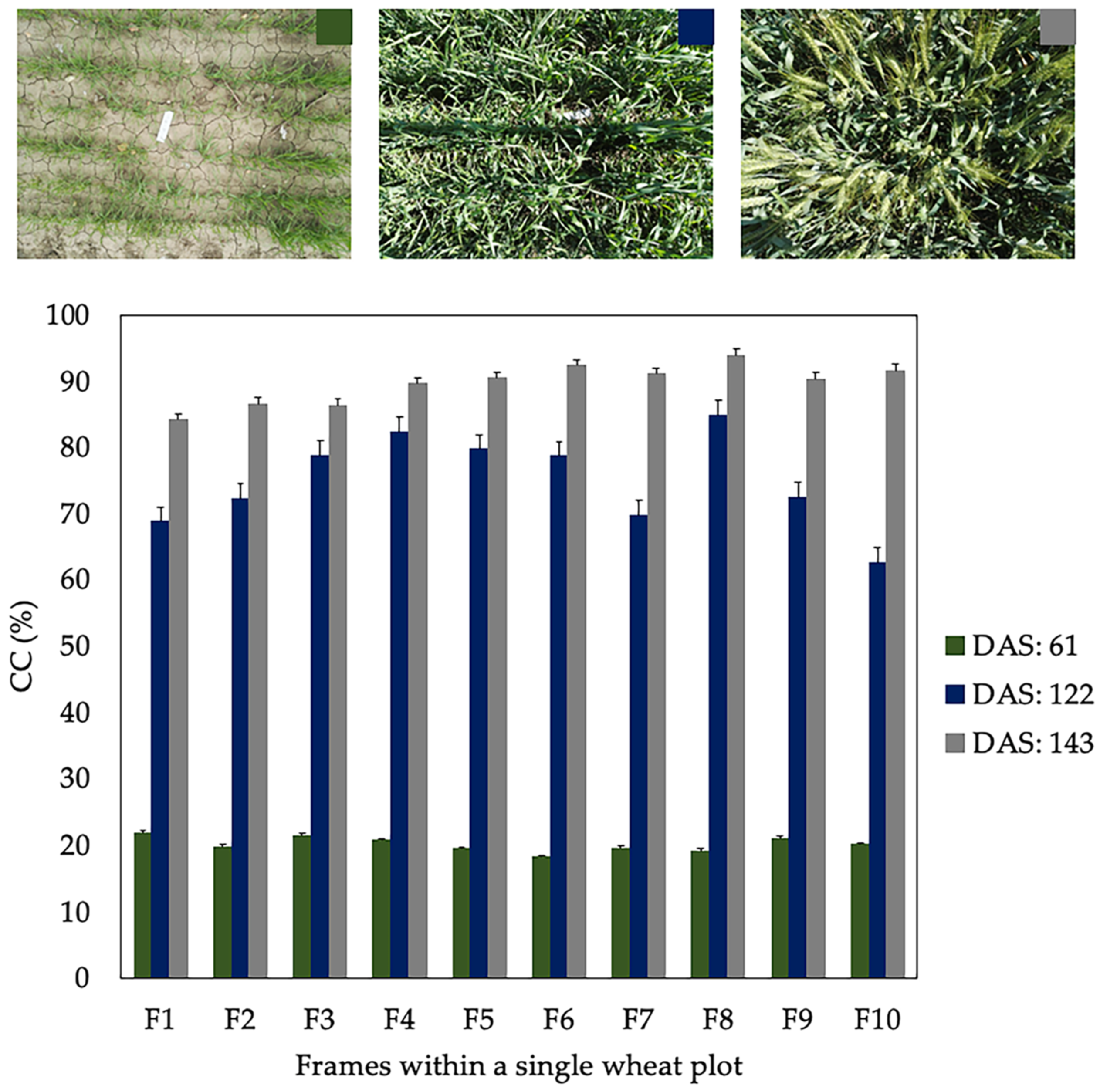
3.2. Spatial Canopy Cover (CC) Variability in a Wheat Plot

According to Sharifi [18] and Jonckheere et al. [19] among others authors cited in the literature, the main disadvantage of image segmentation techniques is their high sensitivity to the changes in light conditions. Figure 7 shows the CC values obtained by analyzing 10 frames of a single wheat plot on different DaS (61, 122 and 143) during the season 2017–18. The standard deviation (SD) of CC for each one of the DaS assessed was 1.13, 6.95 and 3.04 %, respectively. It can be observed that the value of SD is lower when CC is below 30% and notably higher in those DaS with CC greater than 65%. These results show that zones with different CC values can exist within a single wheat plot. These differences are more accentuated as the crop approaches CC values close to 80%, where techniques used for image segmentation have difficulties distinguishing background pixels from those that are actually vegetation. Therefore, we can assume that incorporating several images of the same wheat plot will give greater robustness to the model.

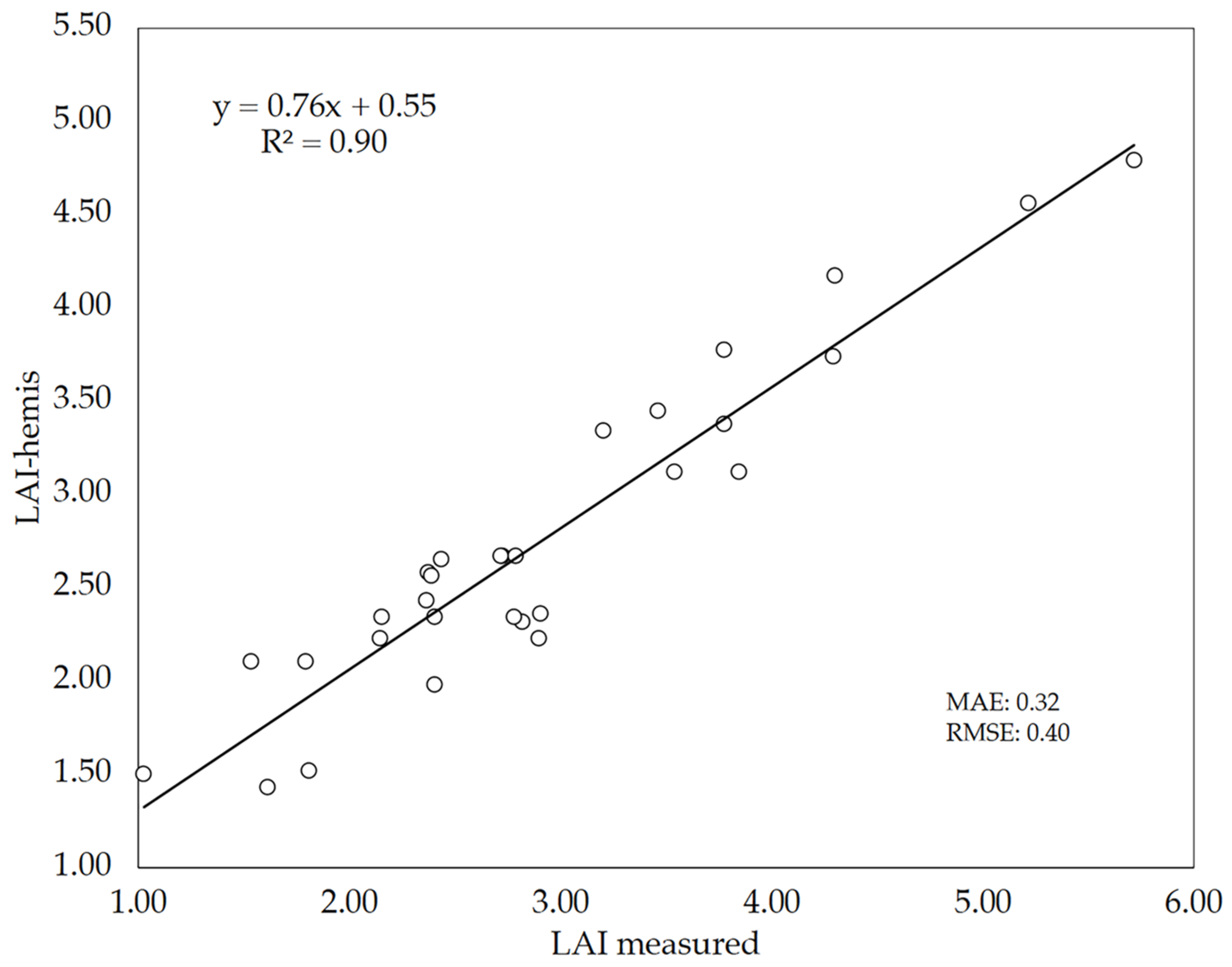
3.3. LAI Estimates Using Bottom-Up Hemispherical Images

The reliability of using bottom-up hemispherical images to estimate the LAI of wheat plots through gap fraction analysis using the Can-Eye software was assessed in 10 wheat cultivars. LAI estimates (True LAI) with this indirect method (LAI-hemis) where evaluated against direct LAI measurements (measured LAI) (Figure 8). The level of agreement between both LAI values was high (R2 = 0.90, MAE = 0.32, RMSE = 0.40), although the indirect method tended to underestimate the LAI values as denoted by the slope of the linear regression (0.76). Other authors already stated that most indirect methods used for LAI estimation generally lead to an underestimation of LAI [62,63], in agreement with our findings. In any case, the LAI values obtained in this study were similar to those observed by Demarez et al. [30] in wheat plants using bottom-up hemispherical images.

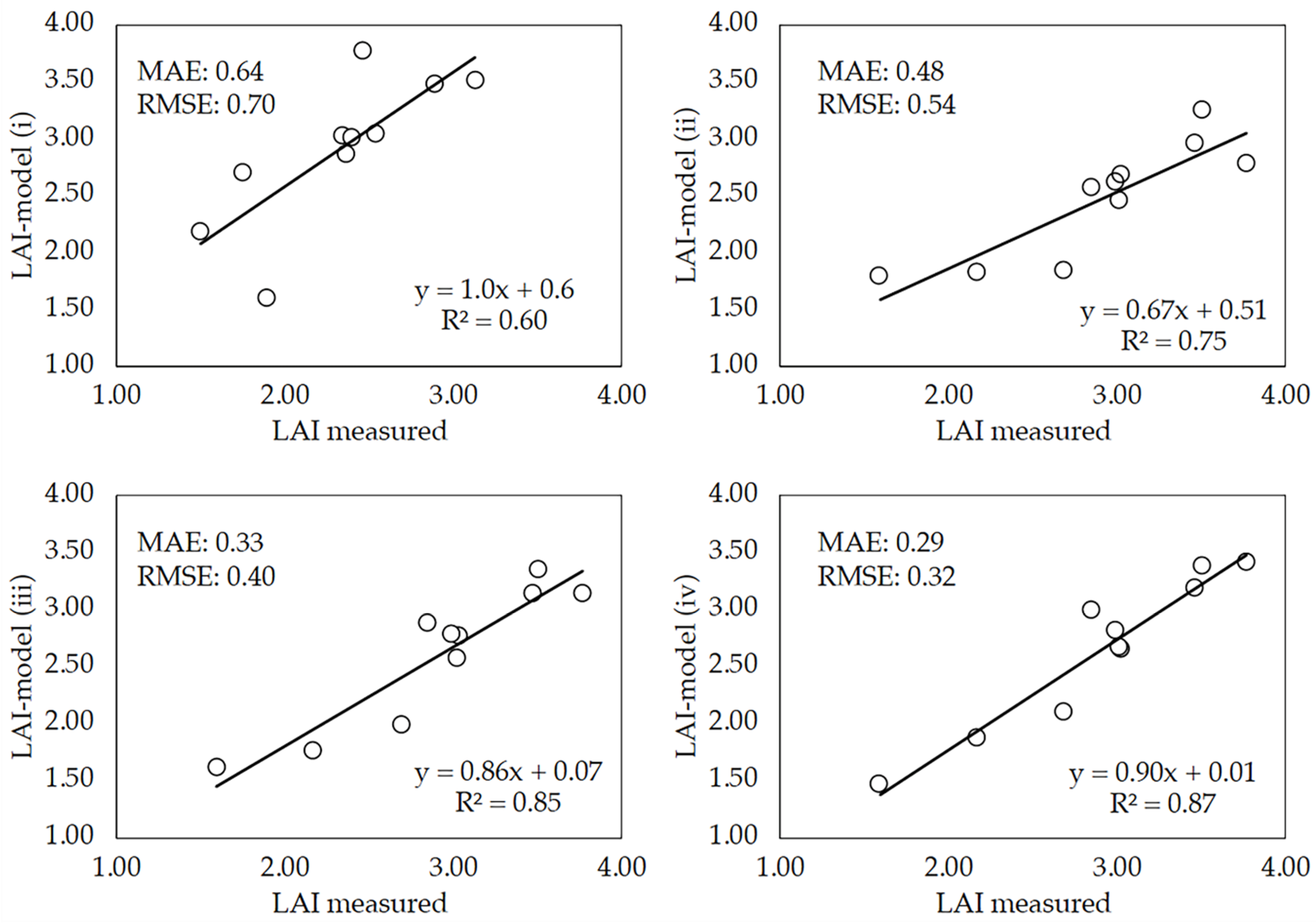
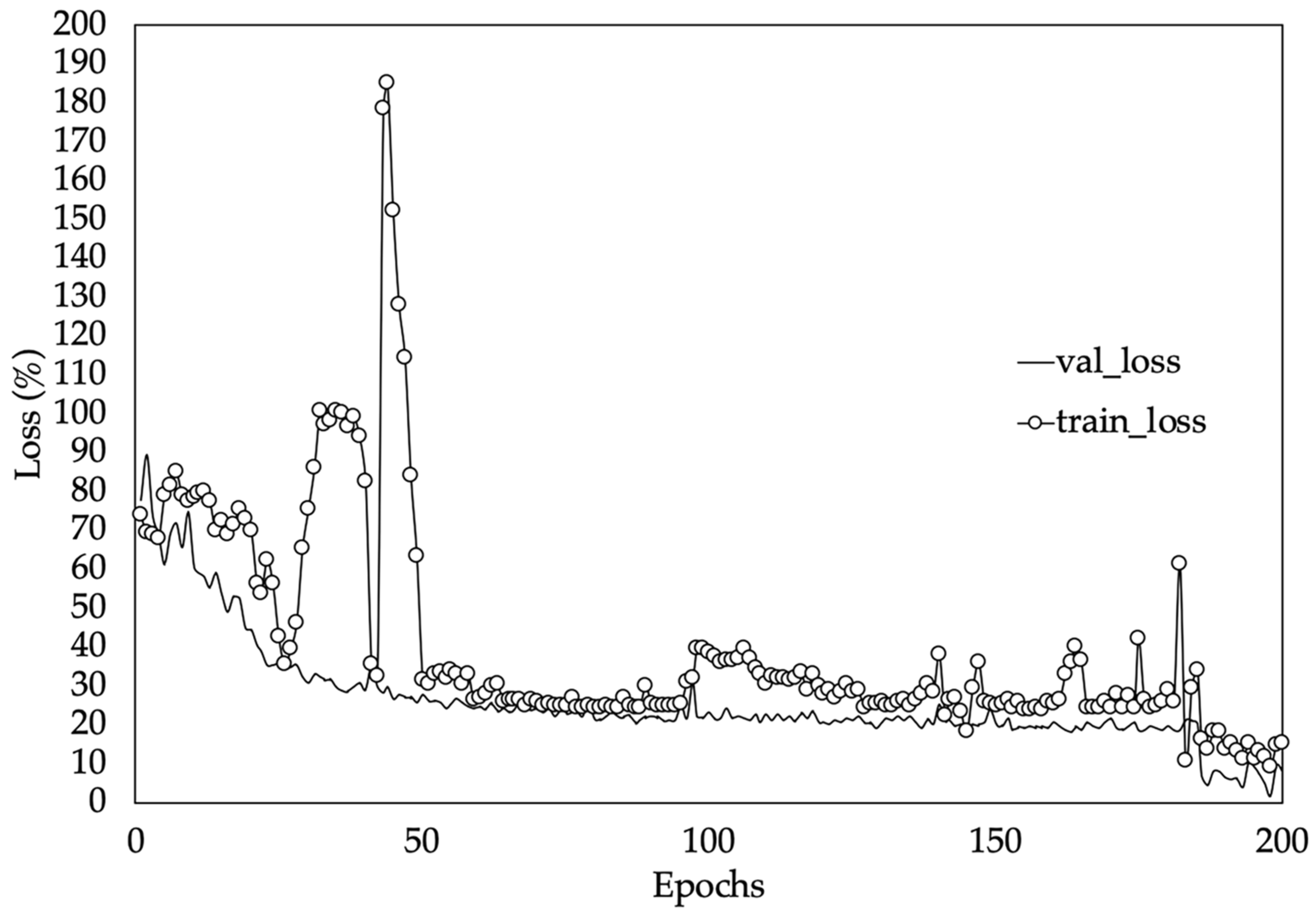
3.4. Performance of the Deep-Learning Model

Although the model can be tested with the percentage (15%) of images randomly split, it was tested with an independent dataset of images taken on DaS 58. This date was selected so that the comparison of the conventional method and the DL model could be performed with images taken on the same day. Of this dataset, 10 images per plot were randomly selected and used to run the four DL model versions previously trained with images and crop traits that were sequentially added as input parameters (see Section 2.5). Figure 9 shows the correlation between LAI measurements (direct method) and LAI estimates made by the four versions of the model (LAI-model). Although the model performed reasonably well when it was trained with images plus CC and LAI values used as inputs, the accuracy of LAI predictions increased as important parameters for the growth and development of wheat were added as inputs for model training. Correlation coefficients higher than 0.6 were obtained with all model versions. However, it was particularly significant when the accuracy increase observed when plant height and the average leaf area of individual wheat leaves were added as inputs for model training. The best performance was achieved when DaS was included as input, achieving a meaningful R2 value of 0.87. Low RMSE and MAE values were observed in all model versions.
Figure 10 shows the training and validation loss (MAPE) values of the best performing model version (iv). Loss values indicate how well or poorly a certain model performs after each iteration of optimization [54]. In this case it can be observed that the mean absolute percentage error started very high but continued to fall throughout the training process. Consequently, at the end of the training process, a loss value of 12.66% on the testing set was obtained. This implies that, on average, the network will be around 13% off in its LAI predictions. In this kind of model where the dataset is made up of different types of data, the weights in the neural network are randomly initialized. Hence, slightly different results will be obtained in terms of MAPE when initialization of weights is poor.
Since 20 images per plot were selected on DaS 58 for validation purposes, another set of 10 different images per plot were used again for LAI estimations, but this time using only LAI-model (iv) (Figure 9). Figure 11 shows the relationship between LAI measurements (direct method) and LAI estimates performed by this version of the model (LAI-model). The results show that the DL model performed reasonably well to predict the LAI of wheat, as denoted by the performance indicators: R2 = 0.81, MAE = 0.39 and RMSE = 0.49. Although these values are somewhat poorer that those obtained previously (Figure 9), it has to be noted that Figure 11 represents the data of the 30 plots evaluated instead of the mean values per cultivar as was done in Figure 9. As compared to the performance of LAI estimations with the hemispherical images and gap fraction theory (Figure 8), the slope of the LAI-model vs. LAI-measured relationship (0.94) indicates that the DL model did not underestimate LAI as previously observed with LAI-hemis. These results suggest that the model can be used as alternative to the hemispherical images, although keeping in mind the errors associated with the model predictions.
Table 4 shows the LAI values measured (direct method) and estimated (DL model and hemispherical images) for 10 wheat cultivars and three replicates per cultivar. The DL model that showed the best performance has been used in the analysis. Statistically significant differences in LAI-measured were observed between THA 3753 and T GALERA. The two indirect methods also found differences between these cultivars although, in their case, significant differences were also found between THA3753 and both TUJENA (LAI-hemis, LAI-model) and MONTALBÁN (LAI-model). Alternatively, a comparison between methods for each cultivar was performed. However, significant differences were not found.

3.5. Novelty of the DL Model against Current Approaches Used for Biophysical Parameters Estimation

Although in terms of accuracy no great differences have been observed between the conventional method (based on using bottom-up hemispherical images) and the DL model, the latter becomes a great alternative to the conventional method for LAI estimation as it requires short processing times. To the best of our knowledge, this is the first study in which a DL model is trained with RGB images and other crop traits for estimating crop biophysical parameters, such as the leaf area index. Different approaches and techniques can be found in the existing literature in which only one type of data (i.e., numerical data or images) is used. For instance, Walter et al. [64] assessed the suitability of using color features in RGB images taken from a HTPP for canopy cover estimations. Their results were satisfactory under greenhouse and field conditions. However, a previous image preprocessing using ImageJ software was used, which increases notably the time required to evaluate multiple cultivars, as is the case in plant breeding programs. Fernández-Gallego [65] also developed an algorithm for a rapid and accurate evaluation of the number of wheat ears as alternative to the manual counts. The method, based mainly on the color features of the images, achieved 90% accuracy with respect to the actual number of ears. Also for wheat, Sadeghi-Tehran et al. [66] developed a deep-learning model for CC estimation using automatic segmentation of RGB images taken on wheat plots. The proposed method was more robust and accurate than other classical and machine-learning methodologies.
Banerjee et al. [67] compared different methods of supervised image classification to estimate LAI in wheat under different soil moisture conditions from two types of images, RGB and thermal. Their results showed that the best estimates were obtained with thermal images and using a support vector machine algorithm. A coefficient of determination of 0.92 was found between estimated LAI and measured LAI with an optical device. They observed a better contrast between vegetation pixels and soil pixels in the thermal image, opening the possibility for future research of using this kind of images as add-on to the RGB images used in this study for estimating crop biophysical traits.
Other LAI estimation methodologies have been developed as alternative to the image-based methodologies. Recently, Feng et al. [68] suggested a new method to estimate LAI in wheat crops when the LAI value is under saturation due to crop growth. The method is based on vegetation indices derived from spectral measurements and explained 78% of the LAI variability observed, slightly lower than the value achieved by the DL model developed in this study. Satellite images have also been used as inputs of an artificial neural network trained with radiative transfer models, PROSPECT (leaf optical properties model) and SAIL (canopy bidirectional reflectance model), to derive LAI maps in winter wheat (Novelli et al. [69]). The authors obtained a coefficient of determination higher than 0.7 in two crop periods after comparing LAI estimates at ground level performed with the optical sensor LAI-2200 Plant Canopy Analyzer and satellite-derived observations. The results were similar to those obtained using the model developed in this paper but, due to the low spatial resolution of satellite images, this methodology is not applicable to the small size of plots in wheat breeding programs. Alternatively, Schirrmann [70] proposed the use of UAV images at low altitude for monitoring biophysical parameters in winter wheat.

3.6. Future Research and Enhancements to Increase the Model Accuracy

The proposed model has shown promising results in terms of accuracy and suitability to be implemented in a high-throughput phenotyping platform. However, the precision of the model and the size of the dataset must be increased in terms of pictures and field data. This is mainly due to the fact that DL models need a huge amount of input data to learn the behavior of patterns across the data. In this study, the growing season lasted 202 and 183 days for each season, respectively. Nevertheless, linear dimensions and pictures used for training the model were only taken during six days. This caused a wide range of LAI values to be unavailable in the dataset. Hence, a greater number of LAI measurements using the allometric relationship, especially during the first stages of crop growth are required. A methodology based on clusters along the plot where leaf measurements can be performed using the allometric relationship developed could improve the accuracy of the model. This approach will increase the number of frames used to train the model and achieve better accuracy in the LAI’s predictions. It is important to highlight that, although the best way to increase the model accuracy is to increase the number of LAI measurements to train the model, adding other biophysical parameters obtained by optical devices (i.e., gaps size, clumping index, etc.) in the training process could also improve the accuracy of the model. Moreover, due to crop growth being influenced by many factors, especially weather conditions (i.e., temperature, relative humidity), the inclusion of these parameters as numerical inputs will be considered in future research.
Finally, the authors consider that this type of image analysis methodology can be transferred rapidly to the sector. The great advantage of the DL-based method, as opposed to the use of hemispheric images, is the difference in processing time of the first (approximately 10 s) as opposed to the second method, which takes approximately 10 min per image [71] and is highly dependent on the operator’s subjectivity [72]. Moreover, the fact that a smartphone has been used as an RGB camera for this work, opens the possibility to develop a mobile application in the future. The DL-based app would be able to estimate LAI from simple RGB images taken with a conventional mobile phone by technicians or plant breeders. Similarly, the use of these models may also be of great interest to derive crop biophysical traits from images taken from aerial platforms such as UAVs for rapid crop phenotyping in commercial and breeding fields.

4. Conclusions

The leaf area index (LAI) is a biophysical trait of great relevance for multiple plant-related disciplines as it describes the plants’ performance under certain environmental conditions. Despite the efforts made over the last decades to develop indirect methods for its estimation in field conditions, precise LAI estimation still presents some challenges in the field of precision agriculture, mainly related to the cost and processing time required by current indirect estimation methods. In this paper a novel technique based on artificial intelligence algorithms and RGB images taken from a high-throughput phenotyping platform (HTPP) has been developed for precise and rapid LAI estimation in wheat breeding plots. The results show that the level of agreement between the model’s LAI outputs and ground truth LAI is high (R2 = 0.81) but slightly lower than that observed with other classical indirect methods for LAI estimation based on gaps theory analysis and hemispherical photography (R2 = 0.90). However, the latter method underestimated LAI values (slope of the regression line of 0.76), while the model developed in this paper predicted LAI values of the same order of magnitude to those that were measured (slope of 0.94). Although the obtained results are promising, the refinement of the algorithms by training the model with an increased dataset that may also include other relevant crop parameters will probably yield better prediction outputs in future works.
This kind of machine-learning model based on inexpensive RGB images opens the possibility of estimating the LAI in wheat breeding fields in a fast (real-time) and economic way, fundamental characteristics for its implementation in affordable high-throughput phenotyping platforms. Further research is still needed to validate its suitability to compute LAI in other crop species.

Supplementary Materials

The following are available online at https://www.mdpi.com/2073-4395/10/2/175/s1, S1: Image segmentation method for nadir-view images using a Python script; S2: Image segmentation method for hemispherical images using Can-Eye software.

Author Contributions

All authors made significant contributions to this manuscript. M.P.-R. and G.E. conceived the experiments and provided guidance for the analysis of data and writing of the manuscript. O.E.A.-A. performed the experiments, wrote the first draft of the paper and analyzed data. J.M.-G. provided suggestions on the experimental design, and participated in the analysis of data and discussion of results. All authors reviewed the manuscript. All authors have read and agreed to the published version of the manuscript.

Funding

This research was supported by the Spanish Ministry of Economy, Industry and Competitiveness (Project: AGL2016-78964-R).

Acknowledgments

The authors are greatly thankful for support from the Predoctoral Research Fellowship for the development of the University of Seville R&D&I program (IV.3 2017) granted to OEAA and the Torres-Quevedo contract (PTQ-17-09506) granted to JMG by the Spanish Ministry of Economy. The authors also thank the company Agrovegetal S.A. (Spain) for allowing the trial to be conducted in its facilities and for the technical support.

Conflicts of Interest

The authors declare that the research was conducted in the absence of any commercial or financial relationships that could be construed as a potential conflict of interest.

References

  1. Foley, J.A.; Ramankutty, N.; Brauman, K.A.; Cassidy, E.S.; Gerber, J.S.; Johnston, M.; Mueller, N.D.; O’Connell, C.; Ray, D.K.; West, P.C.; et al. Solutions for a cultivated planet. Nature 2011, 478, 337–342. [Google Scholar] [CrossRef] [PubMed] [Green Version]
  2. Araus, J.L.; Cairns, J.E. Field high-throughput phenotyping: The new crop breeding frontier. Trends Plant Sci. 2014, 19, 52–61. [Google Scholar] [CrossRef] [PubMed]
  3. Fischer, G. Transforming the global food system. Nature 2018, 562, 501–502. [Google Scholar] [CrossRef] [PubMed]
  4. Bradshaw, J.E. Plant breeding: Past, present and future. Euphytica 2017, 213, 60. [Google Scholar] [CrossRef]
  5. Gonzalez-Dugo, V.; Hernandez, P.; Solis, I.; Zarco-Tejada, P.J. Using high-resolution hyperspectral and thermal airborne imagery to assess physiological condition in the context of wheat phenotyping. Remote Sens. 2015, 7, 13586–13605. [Google Scholar] [CrossRef] [Green Version]
  6. Reynolds, M. Climate Change & Crop Production; CABI: Wallingford, Oxfordshire, UK; Cambridge, MA, USA, 2010; ISBN 9781845936334. [Google Scholar]
  7. Atlin, G.N.; Cairns, J.E.; Das, B. Rapid breeding and varietal replacement are critical to adaptation of cropping systems in the developing world to climate change. Glob. Food Sec. 2017, 12, 31–37. [Google Scholar] [CrossRef]
  8. Lobos, G.A.; Camargo, A.V.; Del Pozo, A.; Araus, J.L.; Ortiz, R.; Doonan, J.H. Editorial: Plant phenotyping and phenomics for plant breeding. Front. Plant Sci. 2017, 8, 1–3. [Google Scholar] [CrossRef] [Green Version]
  9. Chawade, A.; Van Ham, J.; Blomquist, H.; Bagge, O.; Alexandersson, E.; Ortiz, R. High-throughput field-phenotyping tools for plant breeding and precision agriculture. Agronomy 2019, 9, 258. [Google Scholar] [CrossRef] [Green Version]
  10. Mir, R.R.; Reynolds, M.; Pinto, F.; Khan, M.A.; Bhat, M.A. High-throughput phenotyping for crop improvement in the genomics era. Plant Sci. 2019, 282, 60–72. [Google Scholar] [CrossRef]
  11. White, J.W.; Andrade-Sanchez, P.; Gore, M.A.; Bronson, K.F.; Coffelt, T.A.; Conley, M.M.; Feldmann, K.A.; French, A.N.; Heun, J.T.; Hunsaker, D.J.; et al. Field-based phenomics for plant genetics research. Filed Crops Res. 2012, 133, 101–112. [Google Scholar] [CrossRef]
  12. Chapman, S.; Merz, T.; Chan, A.; Jackway, P.; Hrabar, S.; Dreccer, M.; Holland, E.; Zheng, B.; Ling, T.; Jimenez-Berni, J. Pheno-Copter: A Low-Altitude, Autonomous Remote-Sensing Robotic Helicopter for High-Throughput Field-Based Phenotyping. Agronomy 2014, 4, 279–301. [Google Scholar] [CrossRef] [Green Version]
  13. Araus, J.L.; Kefauver, S.C. Breeding to adapt agriculture to climate change: Affordable phenotyping solutions. Curr. Opin. Plant Biol. 2018, 45, 237–247. [Google Scholar] [CrossRef] [PubMed]
  14. Andrade-Sanchez, P.; Gore, M.A.; Heun, J.T.; Thorp, K.R.; Carmo-Silva, A.E.; French, A.N.; Salvucci, M.E.; White, J.W. Development and evaluation of a field-based high-throughput phenotyping platform. Funct. Plant Biol. 2014, 41, 68–79. [Google Scholar] [CrossRef] [Green Version]
  15. Honsdorf, N.; March, T.J.; Berger, B.; Tester, M.; Pillen, K. High-throughput phenotyping to detect drought tolerance QTL in wild barley introgression lines. PLoS ONE 2014, 9, e97047. [Google Scholar] [CrossRef] [Green Version]
  16. Danner, M.; Berger, K.; Wocher, M.; Mauser, W.; Hank, T. Retrieval of Biophysical Crop Variables from Multi-Angular Canopy Spectroscopy. Remote Sens. 2017, 9, 726. [Google Scholar] [CrossRef] [Green Version]
  17. Atzberger, C.; Guérif, M.; Baret, F.; Werner, W. Comparative analysis of three chemometric techniques for the spectroradiometric assessment of canopy chlorophyll content in winter wheat. Comput. Electron. Agric. 2010, 73, 165–173. [Google Scholar] [CrossRef]
  18. Sharifi, A. Estimation of biophysical parameters in wheat crops in Golestan province using ultra-high resolution images. Remote Sens. Lett. 2018, 9, 559–568. [Google Scholar] [CrossRef]
  19. Jonckheere, I.; Fleck, S.; Nackaerts, K.; Muys, B.; Coppin, P.; Weiss, M.; Baret, F. Review of methods for in situ leaf area index determination Part I. Theories, sensors and hemispherical photography. Agric. For. Meteorol. 2004, 121, 19–35. [Google Scholar] [CrossRef]
  20. Zhu, X.; Skidmore, A.K.; Wang, T.; Liu, J.; Darvishzadeh, R.; Shi, Y.; Premier, J.; Heurich, M. Improving leaf area index (LAI) estimation by correcting for clumping and woody effects using terrestrial laser scanning. Agric. For. Meteorol. 2018, 263, 276–286. [Google Scholar] [CrossRef]
  21. Kumar Panguluri, S.; Ashok Kumar, A. Phenotyping for Plant Breeding; Springer: New York, NY, USA, 2013; ISBN 978-1-4614-8319-9. [Google Scholar]
  22. Yan, G.; Hu, R.; Luo, J.; Weiss, M.; Jiang, H.; Mu, X.; Xie, D.; Zhang, W. Review of indirect optical measurements of leaf area index: Recent advances, challenges, and perspectives. Agric. For. Meteorol. 2019, 265, 390–411. [Google Scholar] [CrossRef]
  23. Bonelli, L.E.; Andrade, F.H. Maize radiation use-efficiency response to optimally distributed foliar-nitrogen-content depends on canopy leaf-area index. Field Crops Res. 2019, 5, 107557. [Google Scholar] [CrossRef]
  24. Zhou, B.; Serret, M.D.; Elazab, A.; Bort Pie, J.; Araus, J.L.; Aranjuelo, I.; Sanz-Sáez, Á. Wheat ear carbon assimilation and nitrogen remobilization contribute significantly to grain yield. J. Integr. Plant Biol. 2016, 58, 914–926. [Google Scholar] [CrossRef] [PubMed] [Green Version]
  25. Confalonieri, R.; Foi, M.; Casa, R.; Aquaro, S.; Tona, E.; Peterle, M.; Boldini, A.; De Carli, G.; Ferrari, A.; Finotto, G.; et al. Development of an app for estimating leaf area index using a smartphone. Trueness and precision determination and comparison with other indirect methods. Comput. Electron. Agric. 2013, 96, 67–74. [Google Scholar] [CrossRef]
  26. dos Santos, J.C.C.; Costa, R.N.; Silva, D.M.R.; de Souza, A.A.; de Barros Prado Moura, F.; da Silva Junior, J.M.; Silva, J.V. Use of allometric models to estimate leaf area in Hymenaea courbaril L. Theor. Exp. Plant Physiol. 2016, 28, 357–369. [Google Scholar] [CrossRef]
  27. Comba, L.; Biglia, A.; Ricauda Aimonino, D.; Tortia, C.; Mania, E.; Guidoni, S.; Gay, P. Leaf Area Index evaluation in vineyards using 3D point clouds from UAV imagery. Precis. Agric. 2019, 1–16. [Google Scholar] [CrossRef] [Green Version]
  28. del-Moral-Martínez, I.; Rosell-Polo, J.R.; Company, J.; Sanz, R.; Escolà, A.; Masip, J.; Martínez-Casasnovas, J.A.; Arnó, J. Mapping vineyard leaf area using mobile terrestrial laser scanners: Should rows be scanned on-the-go or discontinuously sampled? Sensors 2016, 16, 119. [Google Scholar] [CrossRef] [Green Version]
  29. Weiss, M.; Baret, F.; Smith, G.J.; Jonckheere, I.; Coppin, P. Review of methods for in situ leaf area index (LAI) determination. Agric. For. Meteorol. 2004, 121, 37–53. [Google Scholar] [CrossRef]
  30. Demarez, V.; Duthoit, S.; Baret, F.; Weiss, M.; Dedieu, G. Estimation of leaf area and clumping indexes of crops with hemispherical photographs. Agric. For. Meteorol. 2008, 148, 644–655. [Google Scholar] [CrossRef] [Green Version]
  31. Gonsamo, A.; Walter, J.M.; Chen, J.M.; Pellikka, P.; Schleppi, P. A robust leaf area index algorithm accounting for the expected errors in gap fraction observations. Agric. For. Meteorol. 2018, 248, 197–204. [Google Scholar] [CrossRef]
  32. Liu, S.; Baret, F.; Abichou, M.; Boudon, F.; Thomas, S.; Zhao, K.; Fournier, C.; Andrieu, B.; Irfan, K.; Hemmerlé, M.; et al. Estimating wheat green area index from ground-based LiDAR measurement using a 3D canopy structure model. Agric. For. Meteorol. 2017, 247, 12–20. [Google Scholar] [CrossRef]
  33. Li, Y.; Guo, Q.; Su, Y.; Tao, S.; Zhao, K.; Xu, G. Retrieving the gap fraction, element clumping index, and leaf area index of individual trees using single-scan data from a terrestrial laser scanner. ISPRS J. Photogramm. Remote Sens. 2017, 130, 308–316. [Google Scholar] [CrossRef]
  34. Woodgate, W.; Jones, S.D.; Suarez, L.; Hill, M.J.; Armston, J.D.; Wilkes, P.; Soto-Berelov, M.; Haywood, A.; Mellor, A. Understanding the variability in ground-based methods for retrieving canopy openness, gap fraction, and leaf area index in diverse forest systems. Agric. For. Meteorol. 2015, 205, 83–95. [Google Scholar] [CrossRef]
  35. Ubbens, J.R.; Stavness, I. Deep plant phenomics: A deep learning platform for complex plant phenotyping tasks. Front. Plant Sci. 2017, 8. [Google Scholar] [CrossRef] [PubMed] [Green Version]
  36. Chen, C.H.; Kung, H.Y.; Hwang, F.J. Deep learning techniques for agronomy applications. Agronomy 2019, 9, 142. [Google Scholar] [CrossRef] [Green Version]
  37. Lu, J.; Hu, J.; Zhao, G.; Mei, F.; Zhang, C. An in-field automatic wheat disease diagnosis system. Comput. Electron. Agric. 2017, 142, 369–379. [Google Scholar] [CrossRef] [Green Version]
  38. Hasan, M.M.; Chopin, J.P.; Laga, H.; Miklavcic, S.J. Detection and analysis of wheat spikes using Convolutional Neural Networks. Plant Methods 2018, 14, 1–13. [Google Scholar] [CrossRef] [Green Version]
  39. Ma, J.; Li, Y.; Chen, Y.; Du, K.; Zheng, F.; Zhang, L.; Sun, Z. Estimating above ground biomass of winter wheat at early growth stages using digital images and deep convolutional neural network. Eur. J. Agron. 2019, 103, 117–129. [Google Scholar] [CrossRef]
  40. Durbha, S.S.; King, R.L.; Younan, N.H. Support vector machines regression for retrieval of leaf area index from multiangle imaging spectroradiometer. Remote Sens. Environ. 2007, 107, 348–361. [Google Scholar] [CrossRef]
  41. Jin, X.; Li, Z.; Feng, H.; Ren, Z.; Li, S. Deep neural network algorithm for estimating maize biomass based on simulated Sentinel 2A vegetation indices and leaf area index. Crop J. 2019. [Google Scholar] [CrossRef]
  42. Houborg, R.; McCabe, M.F. A hybrid training approach for leaf area index estimation via Cubist and random forests machine-learning. ISPRS J. Photogramm. Remote Sens. 2018, 135, 173–188. [Google Scholar] [CrossRef]
  43. Gebremedhin, A.; Badenhorst, P.E.; Wang, J.; Spangenberg, G.C.; Smith, K.F. Prospects for measurement of dry matter yield in forage breeding programs using sensor technologies. Agronomy 2019, 9, 65. [Google Scholar] [CrossRef] [Green Version]
  44. Tsaftaris, S.A.; Minervini, M.; Scharr, H. Machine Learning for Plant Phenotyping Needs Image Processing. Trends Plant Sci. 2016, 21, 989–991. [Google Scholar] [CrossRef] [PubMed] [Green Version]
  45. Shafian, S.; Rajan, N.; Schnell, R.; Bagavathiannan, M.; Valasek, J.; Shi, Y.; Olsenholler, J. Unmanned aerial systems-based remote sensing for monitoring sorghum growth and development. PLoS ONE 2018, 13, e0196605. [Google Scholar] [CrossRef] [PubMed] [Green Version]
  46. Lonsdon, S.D.; Cambardella, C.A. An approach for indirect determination of leaf area index. Am. Soc. Agric. Biol. Eng. 2019, 62, 655–659. [Google Scholar] [CrossRef]
  47. Ahmad, S.; Rehman, A.U.; Irfan, M.; Khan, M.A. Measuring Leaf Area of Winter Cereals by Different Techniques: A Comparison. Pak. J. Life Soc. Sci. 2015, 13, 117–125. [Google Scholar]
  48. Barhoumi, W.; Zagrouba, E. On-the-fly Extraction of Key Frames for Efficient Video Summarization. AASRI Procedia 2013, 4, 78–84. [Google Scholar] [CrossRef]
  49. Rosebrock, A. Practical Python and OpenCV + Case Studies; PyImageSearch.com: Baltimore, MD, USA, 2016. [Google Scholar]
  50. Urban, S.; Leitloff, J.; Hinz, S. Improved wide-angle, fisheye and omnidirectional camera calibration. ISPRS J. Photogramm. Remote Sens. 2015, 108, 72–79. [Google Scholar] [CrossRef]
  51. Gulli, A.; Pal, S. Deep Learning with Keras; Packt Publishing: Birmingham, UK; Volume 73, ISBN 978-1-78712-842-2.
  52. Chollet, F. Keras. Available online: https://keras.io (accessed on 5 September 2019).
  53. Manaswi, N.K. Deep Learning with Applications Using Python; Apress: Bangalore, India, 2018; ISBN 9781484235164. [Google Scholar]
  54. Rosebrock, A. Deep Learning for Computer Vision with Python. ImageNet Bundle; PyImageSearch.com: Baltimore, MA, USA, 2018. [Google Scholar]
  55. Kingma, D.P.; Ba, J.L. Adam: A method for stochastic optimization. In Proceedings of the 3rd International Conference on Learning Representations (ICLR2015), San Diego, CA, USA, 7–9 May 2015; pp. 1–15. [Google Scholar]
  56. Bradski, G. The opencv library (2000). Dr. Dobb’s J. Softw. Tools 2000. Available online: https://opencv.org/ (accessed on 5 June 2019).
  57. Team, R.S. RStudio: Integrated Development for R; RStudio Inc.: Boston, MA, USA, 2016; Available online: https://www.rstudio.com/ (accessed on 30 October 2019).
  58. David R Legates, G.J.M. Evaluating the use of “goodness-of-fit” measures in hydrologic and hydroclimatic model validation. Water Resour. Res. 2007, 35, 1–9. [Google Scholar]
  59. Chanda, S.V.; Singh, Y.D. Estimation of leaf area in wheat using linear measurements. Plant Breed. Seed Sci. 2002, 46, 75–79. [Google Scholar]
  60. Calderini, D.F.; Miralles, D.J.; Sadras, V.O. Appearance and growth of individual leaves as affected by semidwarfism in isogenic lines of wheat. Ann. Bot. 1996, 77, 583–589. [Google Scholar] [CrossRef]
  61. Bryson, R.J.; Paveley, N.D.; Clark, W.S.; Slylvester-Bradley, R.; Scott, R.K. Use of in-field measurements of green leaf area and incident radiation to estimate the effects of yellow rust epidemics on the yield of winter wheat. Dev. Crop Sci. 1997, 25, 77–86. [Google Scholar] [CrossRef]
  62. Stroppiana, D.; Boschetti, M.; Confalonieri, R.; Bocchi, S.; Brivio, P.A. Evaluation of LAI-2000 for leaf area index monitoring in paddy rice. Field Crops Res. 2006, 99, 167–170. [Google Scholar] [CrossRef]
  63. Bréda, N.J.J. Ground-based measurements of leaf area index: A review of methods, instruments and current controversies. J. Exp. Bot. 2003, 54, 2403–2417. [Google Scholar] [CrossRef]
  64. Walter, J.; Edwards, J.; Cai, J.; McDonald, G.; Miklavcic, S.J.; Kuchel, H. High-throughput field imaging and basic image analysis in a wheat breeding programme. Front. Plant Sci. 2019, 10. [Google Scholar] [CrossRef]
  65. Fernandez-Gallego, J.A.; Kefauver, S.C.; Gutiérrez, N.A.; Nieto-Taladriz, M.T.; Araus, J.L. Wheat ear counting in-field conditions: High throughput and low-cost approach using RGB images. Plant Methods 2018, 14, 1–12. [Google Scholar] [CrossRef] [Green Version]
  66. Sadeghi-Tehran, P.; Virlet, N.; Sabermanesh, K.; Hawkesford, M.J. Multi-feature machine learning model for automatic segmentation of green fractional vegetation cover for high-throughput field phenotyping. Plant Methods 2017, 13, 1–16. [Google Scholar] [CrossRef] [Green Version]
  67. Banerjee, K.; Krishnan, P.; Mridha, N. Application of thermal imaging of wheat crop canopy to estimate leaf area index under different moisture stress conditions. Biosyst. Eng. 2018, 166, 13–27. [Google Scholar] [CrossRef]
  68. Feng, W.; Wu, Y.; He, L.; Ren, X.; Wang, Y.; Hou, G.; Wang, Y.; Liu, W.; Guo, T. An optimized non-linear vegetation index for estimating leaf area index in winter wheat. Precis. Agric. 2019, 20, 1157–1176. [Google Scholar] [CrossRef] [Green Version]
  69. Novelli, F.; Vuolo, F. Assimilation of sentinel-2 leaf area index data into a physically-based crop growth model for yield estimation. Agronomy 2019, 9, 255. [Google Scholar] [CrossRef] [Green Version]
  70. Schirrmann, M.; Giebel, A.; Gleiniger, F.; Pflanz, M.; Lentschke, J.; Dammer, K.H. Monitoring agronomic parameters of winter wheat crops with low-cost UAV imagery. Remote Sens. 2016, 8, 706. [Google Scholar] [CrossRef] [Green Version]
  71. Weiss, M.; Baret, F. Can_Eye V6.4.91 User Manual. Available online: https://www6.paca.inra.fr/can-eye/News/CAN-EYE-V6.49-Release (accessed on 9 May 2019).
  72. Duveiller, G.; Defourny, P. Batch processing of hemispherical photography using object-based image analysis to derive canopy biophysical variables. In Proceedings of the GEOBIA 2010: Geographic Object-Based Image Analysis, Ghent, Belgium, 29 June–2 July 2010; Volume XXXVIII-4/C7. [Google Scholar]
Figure 1. Aerial view of the experimental site (a), aerial image of the wheat breeding trial (b), details of a few individual plots (c).
Agronomy 10 00175 g001
Figure 2. Data collection process for building the allometric relationship. Leaves stored in plastic bags to be transported in a cooler (a); measurements of the unitary leaf area using the LICOR-3100 (b); and leaves placed on a sheet of paper with the squares in the background (c).
Agronomy 10 00175 g002
Figure 3. Methodology for measuring plant height.
Agronomy 10 00175 g003
Figure 4. Image acquisition using the high-throughput phenotyping platform (HTPP). (a) A picture of the HTPP platform working in the field. A detail of the way the device was attached to the HTPP and a frame taken with the smartphone are shown in (b) and (c), respectively.
Agronomy 10 00175 g004
Figure 5. The device (Go Pro camera) used to take the bottom-up hemispherical images during the study (b) and an example of the resulting images (a).
Agronomy 10 00175 g005
Figure 6. Artificial neural network architecture for leaf area index (LAI) estimation using visual features and crop parameters as numerical inputs.
Agronomy 10 00175 g006
Figure 7. Canopy cover (CC) values for 10 frames within a single wheat plot on different days after sowing (DaS) during 2017–18 season. The error bars represent the standard deviation (SD) of the data.
Agronomy 10 00175 g007
Figure 8. Relationship between measured LAI (direct method) and LAI estimated by bottom-up hemispherical images (LAI-hemis). The number of plots analyzed was n = 30. The straight line represents the best-fit linear regression (p < 0.001).
Agronomy 10 00175 g008
Figure 9. Linear regressions between measured LAI (direct method) and LAI estimates made by the four model versions (LAI-model). LAI-model (i): the model was trained using only red green blue (RGB) images, canopy cover (CC) value and LAI; LAI-model (ii): the plant height was added as additional parameter together with those previously used; LAI-model (iii): the mean leaf area of individual wheat leaves was added; LAI-model (iv): the days after sowing (DaS) was included as an input to train the model. Each point is the mean of three replicates per wheat cultivar.
Agronomy 10 00175 g009
Figure 10. Training and validation loss values on dataset. Validation loss (val_loss) and training loss (train_loss).
Agronomy 10 00175 g010
Figure 11. Relationship between LAI estimated by the deep-learning (DL) model (LAI-model) and measured LAI (direct method).
Agronomy 10 00175 g011
Table 1. Dates of measurements and imagery acquisition during the trial seasons.
DatesDaSSeason
25 January61 a2017–2018
27 March1222017–2018
17 April1432017–2018
2 February58 a,b2018–2019
14 February702018–2019
25 February812018–2019
29 March1132018–2019
a Destructive leaf area index (LAI) measurements were performed on these dates. b On this day, bottom-up hemispherical images were also taken. DaS: days after sowing.
Table 2. Technical features of each one of the cameras used in this study.
Technical FeaturesGoProHuawei P8
ModelHERO3 + Black EditionHUAWEI GRA-UL10
Weight (g)74144
Sensor typeCMOS cCMOS c
Sensor size6.17 × 4.554.62 × 6.16
Pixel size (µm)1.551.12
Image/video resolution4000 × 30001920 × 1080
Focal length (mm)2.773.83
Output formatJPGMP4
c CMOS (complementary metal-oxide semiconductor) sensors utilize Bayer color filter mosaic arrays.
Table 3. Allometric relationships between L*W (product of length and maximum leaf width) and leaf area of individual wheat leaves (LA).
SeasonDaSRegression EquationR2Standard Error
[cm2]
No. of Observations
2017–1861LA = 0.75LW − 0.900.910.24411
2018–1858LA = 0.78LW + 0.500.940.41855
CombinedLA = 0.71LW + 0.920.940.091266
DaS: Days after sawing when the leaves were collected. All the relationships were significant at p < 0.001.
Table 4. LAI values determined for ten wheat cultivars with the direct and the two indirect methods assessed in this study during DaS = 58 (2 February 2019).
Wheat CultivarLAI-MeasuredSDLAI-HemisSDLAI-ModelSD
THA 37531.59a0.561.72a0.441.52a0.32
CONIL2.17ab0.652.25ab0.132.02ab0.51
T GAZUL2.69ab0.282.54ab0.163.10ab0.44
MARCHENA2.85ab0.922.59ab0.662.54ab1.07
THA 38292.99ab0.762.78ab0.573.23ab1.08
ANTEQUERA3.02ab1.112.85ab0.723.43ab0.97
VALBONA3.03ab0.382.91ab0.623.44ab0.77
MONTALBÁN3.47ab1.533.08ab1.283.50b1.00
TUJENA3.51ab0.963.36b0.763.63b1.11
T GALERA3.77b1.963.40b1.673.83b1.87
SD: standard deviation. LAI-measured: LAI obtained by the direct approach, LAI-hemis: LAI estimates using hemispherical images and LAI-model: LAI estimates using the DL model developed. Within the same column, different letters indicate statistically significant differences according to the Duncan’s multiple range test (p < 0.05).

