Article

Within-Field Relationships between Satellite-Derived Vegetation Indices, Grain Yield and Spike Number of Winter Wheat and Triticale

1
Department of Biometry, Warsaw University of Life Sciences, Nowoursynowska 159, 02-776 Warsaw, Poland
2
Complex of Agricultural Schools, Grzybno 48, 63-112 Brodnica, Poland
3
Department of Agronomy, Warsaw University of Life Sciences, Nowoursynowska 159, 02-776 Warsaw, Poland
4
Wasat Sp. z o.o., Office in Gdansk, Science and Technology Park, Trzy Lipy 3, 80-172 Gdansk, Poland
*
Author to whom correspondence should be addressed.
Agronomy 2020, 10(11), 1842; https://doi.org/10.3390/agronomy10111842
Submission received: 14 October 2020 / Revised: 10 November 2020 / Accepted: 19 November 2020 / Published: 23 November 2020
(This article belongs to the Special Issue Site-Specific Nutrient Management)

Abstract

:
The aims of this study were to: (i) evaluate the relationships between vegetation indices (VIs) derived from Sentinel-2 imagery and grain yield (GY) and the number of spikes per square meter (SN) of winter wheat and triticale; (ii) determine the dates and plant growth stages when the above relationships were the strongest at individual field scale, thus allowing for accurate yield prediction. Observations of GY and SN were performed at harvest on six fields (three locations in two seasons: 2017 and 2018) in three regions of Poland, i.e., northeastern (A—Brożówka), central (B—Zdziechów) and southeastern Poland (C—Kryłów). Vegetation indices (Normalized Difference Vegetation Index (NDVI), Soil-Adjusted Vegetation Index (SAVI), modified SAVI (mSAVI), modified SAVI 2 (mSAVI2), Infrared Percentage Vegetation Index (IPVI), Global Environmental Monitoring Index (GEMI), and Ratio Vegetation Index (RVI)) calculated for sampling points from mid-March until mid-July, covering within-field soil and topographical variability, were included in the analysis. Depending on the location, the highest correlation coefficients (of about 0.6–0.9) for most of VIs with GY and SN were obtained about 4–6 weeks before harvest (from the beginning of shooting to milk maturity). Therefore, satellite-derived VIs are useful for the prediction of within-field cereal GY as well as SN variability. Information on GY, predicted together with the results for soil nutrient availability, is the basis for the formulation of variable fertilize rates in precision agriculture. All examined VIs were similarly correlated with GY and SN via the commonly used NDVI. The increase in NDVI by 0.1 unit was related to an average increase in GY by about 2 t ha−1.

1. Introduction

Satellite remote sensing (RS) helps in the mapping of current crop status and the assessment of biophysical parameters. Currently, RS data are publicly accessible due to the availability of an unprecedented amount of Free Sentinel data from the Copernicus Program, established by the European Space Agency [1]. Constellations of the Sentinel-2 satellites (2A and 2B) can be also used for precision farming applications [2]. Thanks to the high spatial resolution (pixel size of 10 m), relatively short revisit time (about 5 days) and multispectral sensors, it is possible to observe and analyze the crop status using vegetation indices (VIs). For the purpose of such an evaluation, satellite Sentinel-2 images of two radiation bands, red (650–680 nm) and NIR (785–900 nm), are usually used [2].
Recently, many research results on yield evaluation based on data from the Sentinel-2 satellites [3,4,5,6,7,8] as well as from other satellite sources has been available. However, studies in which significant relationships between NDVI and the grain yield of cereals were proved have been carried out since the 1980s [3,4,5,6]. Most of these studies were done at a regional level and low-resolution satellite imagery was used (mainly using AVHRR/NOAA - Advanced Very High Resolution Radiometer/National Oceanic and Atmospheric Administration sensors with pixel sizes of 1 km).
Research on the evaluation of the relationships between VIs from high-resolution satellite sensors (e.g., QuickBird) and the grain yield and crop status of cereals has become more common since the year 2000 [7,8,9,10], due to the availability of new sources of satellite data. Such of studies were conducted at different spatial scales from one field scale (evaluation of within-field yield variability) to a whole country level. Many studies refer to Vis in relation to wheat grain yield because of the high importance of this crop. In most studies, Normalized Difference Vegetation Index (NDVI) [5] has been used as a predictor of grain yield. The highest accuracy of grain yield forecast was possible at different growth stages, even 2–3 months before harvest [11,12,13,14,15,16]. Recently, other VIs besides NDVI have been used as grain yield predictors. Ali et al. (2019) [17] studied the relationship between six vegetation indices (NDVI, EVI—Enhanced Vegetation Index, SAVI—Soil-Adjusted Vegetation Index, GNDVI—Green Normalized Vegetation Index, GCI—Green Chlorophyll Index and SR—Simple Ratio), derived from Landsat 5, 7 and 8 satellite imagery and a grain yield of durum and bread wheat in one 11 ha field in Italy, during five consecutive years (2010–2014). Most frequently, NDVI and SR were characterized as having the strongest relationship with yields.
Most of the studies that examined relationships between satellite-derived VIs and the grain yield of cereals were conducted at a regional level and did not analyze the relationships of VIs with other yield components such as the number of spikes. Nowadays, the common availability of satellite images of relatively high spatial resolution allows us to evaluate these relationships even at the within-field level. The results of such an evaluation can be useful for site-specific crop management, including variable fertilization, which should be based, besides soil nutrient availability, on the prediction of grain yields.
The aim of this study was to evaluate the relationships between vegetation indices derived from Sentinel-2 imagery and grain yield and the number of spikes per square meter of winter wheat and triticale. These two crops were selected because of their high cropping area among cereals in Poland. Recently, winter wheat has been grown on about 1.9 M hectares and winter triticale on 1.1 M hectares [18]. Moreover, the aim was to determine the dates and plant growth stages when the above relationships were the strongest at the individual field scale, thus allowing an accurate yield prediction.

2. Materials and Methods
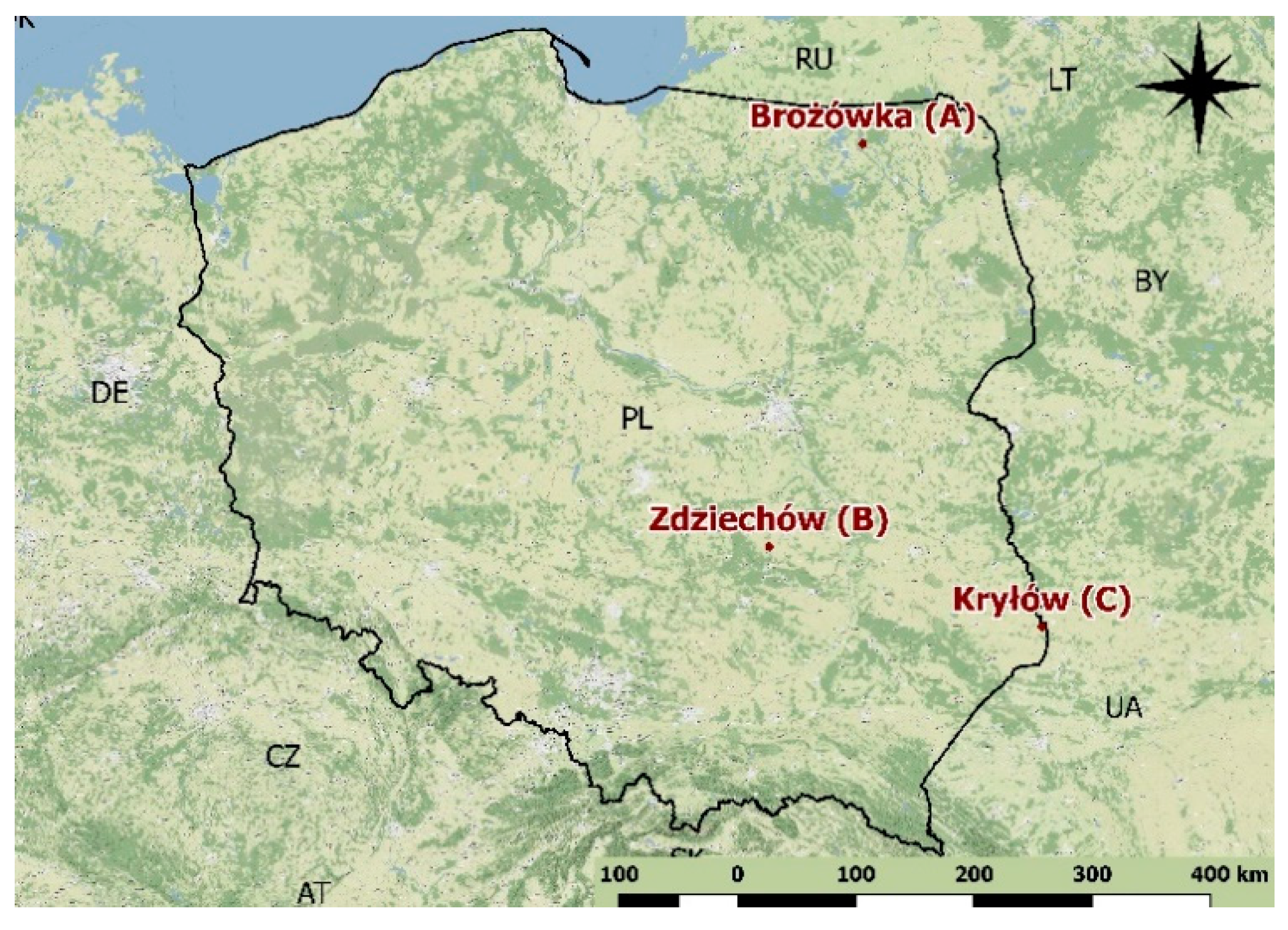
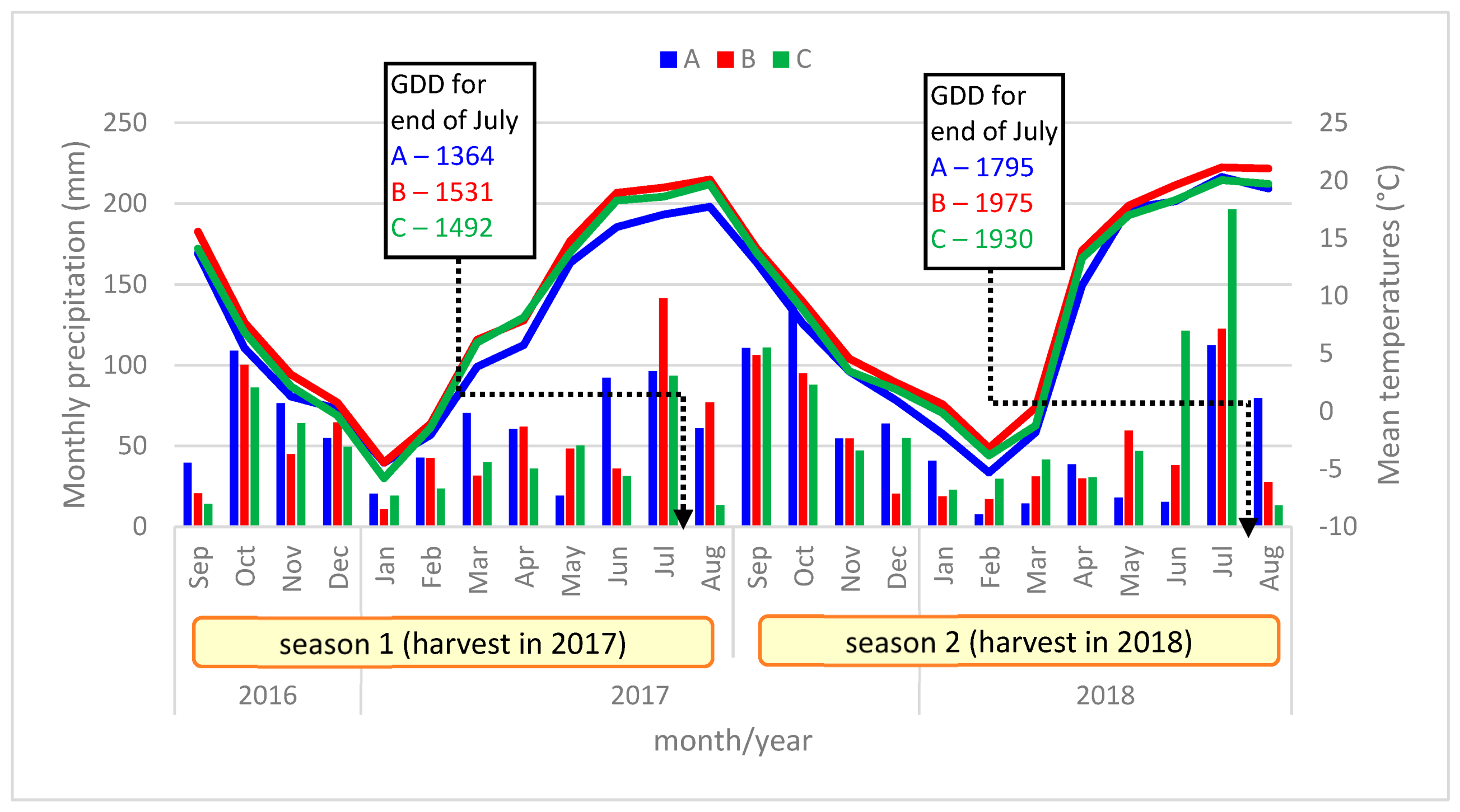
2.1. Study Area

Three research sites cropped with winter wheat (Triticum aestivum L.) or winter triticale (Triticosecale Witt.) (Table 1) were located in Brożówka, northern Poland, in the land of the Great Masurian Lakes (location A), in Zdziechów, central Poland, in the Mazowieckie Voivodeship (location B), and in Kryłów, southeast Poland, close to the border with Ukraine (location C) (Figure 1).
According to the Köppen classification [19], the majority of Poland lies in the warm temperate climate zone with fully humid continental climate and hot summers (Cfb). The locations of Kryłów (C) and Zdziechów (B) are situated within this zone, while the location of Brożówka (A) is placed in the transitional area between the Cfb zone and the snowy climate zone, with fully humid and warm summers (Dfb).
The sum of precipitation in two studied seasons (from the beginning of September to the end of August) ranged from about 520 mm (location C, season 2016/2017) to 740 mm (location A, season 2016/2017). The lowest air temperatures were observed for location A, while locations B and C were characterized by similar air temperatures. Growing degree days calculated at a base air temperature of 5 °C for the period from the sowing date to the end of July were much lower in 2017 (for locations: A—1364, B—1531, and C—1492) in comparison to 2018 (for locations: A—1795, B—1975, and C—1930). Monthly sums of precipitation and mean air temperatures for the nearest meteorological stations from the Institute of Meteorology and Water Management National Research Institute IMGW-PIB (https://danepubliczne.imgw.pl/) are presented in the Figure 2.

2.2. Soil and Plant Sampling

Within each of the fields, sampling points of soil and plants were georeferenced using a Global Positioning System (GPS) receiver. The locations of the sampling points were selected to obtain large variability in the studied traits, i.e., soil properties as well grain yield and ear number (Figure 3). The characteristics of each of the three research sites are presented in Table 1.
Soil samples were collected from a layer of 0–90 cm at the end of winter or in early spring before the starting of the vegetation. Grain yield and number of ears per square meter were determined at the full maturity of plants in plots of 2 m2 (2 × 1 m2 subplots, each located very closely to the soil and plant sampling points). The following statistical parameters were calculated: average, standard deviation, minimum, and maximum for each field in a given year.

2.3. Satellite Data

Satellite Sentinel-2 (2A and 2B) images of Level-1C with a spatial resolution of 10 to 20 m in the range of visible and near-infrared (NIR—band 8 at central wavelength 833 nm) light were downloaded from the Copernicus Open Access Hub [20]. Level-1C processing includes radiometric and geometric corrections, namely ortho-rectification and spatial registration, on a global reference system with a sub-pixel accuracy. Then, the acquired Level 1C products were subjected to atmospheric correction using the Dark Object Subtraction (DOS1) method in Semi-Automatic Classification Plugin documentation (SCP), developed by Luca Congedo (2016) [21].
Vegetation indices were derived for the representative soil and plant sampling points established within fields and imported together with the coordinates of these points. Then, they were compiled into tables and subjected to regression analyses. Depending on the location, despite the revisit time of about 5 days, it was only possible to acquire cloudless satellite images during the intensive growth of cereals in spring and early summer for 4–6 dates (Table 2).

2.4. Spectral Vegetation Indices

The selection of the vegetation indices (VIs) used for the winter wheat and triticale yield analysis depended on several factors. First of all, we only considered the same satellite data spatial resolution. Another factor determining our choices was the prevalence in the literature and the comparability with the yield of cereal crops. The VIs were calculated on the basis of the reflectance of wavelength bands registered by Sentinel-2 at spatial resolution 10 m (squared pixels 10 × 10 m). The Normalized Differential Vegetation Index (NDVI) allows us to determine the indirect absorption of photosynthetic radiation on a landscape scale. NDVI calculation is based on the contrast between the largest reflection in the near-infrared band and the absorption in the red band. In the case of this index, the difference in reflection in the near-infrared and red bands is divided by their sum. This approach compensates for the differences in the radiation amounts in both bands. It is believed that NDVI is more sensitive to small amounts of vegetation [22,23].
NDVI = NIR     RED NIR + RED
Another VI used in this study was the Soil-Adjusted Vegetation Index (SAVI). This indicator was designed to minimize the effect of soil reflection on red and near-infrared radiation by adding an estimated background correction factor [24].
SAVI = ( 1 + L ) ( NIR     RED ) NIR + RED + L
where L is a canopy background adjustment factor. An L value of 0.5 was adopted to minimize soil brightness variations and eliminate the need for additional calibration for different soils.
In the literature, modifications of the SAVI index, known as modified SAVI (mSAVI) and modified SAVI 2 (mSAVI2), are often used. These two VIs also include the soil background correction factor [25]:
mSAVI = ( 1 + L ) ( NIR     RED ) NIR + RED + L
where L is:
L = 1 2 × s   × ( NIR s × RED ) ( NIR     RED ) NIR + RED ,
and:
mSAVI 2 = ( 2 × NIR + 1 ( 2 × N I R + 1 ) 2 8 × ( NIR RED ) 2
Crippen (1990) proposed the Infrared Percentage Vegetation Index (IPVI), which simplifies the calculation by eliminating the subtraction of the red radiation value in the NDVI indicator counter. This simplification of a new VI calculation proved to be important for fast image processing [26].
IPVI = NIR NIR + RED
In 1992, Pinty and Verstraete proposed the Global Environmental Monitoring Index (GEMI), a new nonlinear crop status indicator, which includes a correction factor adjusted by the effect of soil reflectance and atmospheric background [27].
GEMI = n ( 1 0.25 n ) RED 0.125 1 RED
where:
n = [ 2 × ( NIR 2 R 2 ) + 1.5 NIR + 0.5 R ] NIR + RED + 0.5
The last VI used in this study for a comparison with NVDI was the Ratio Vegetation Index (RVI), sometimes also referred to as the Simple Ratio (SR). This VI is a ratio of NIR and red reflectance [28].
RVI = NIR RED
The investigated Vis, except RVI, are normalized and placed on a comparative scale. These indices have values from −1 to 1, where values close to −1 indicate water, or any inanimate matter, values from 0 to 0.20 relate to barren rock, sand, barren soil and plants at an early stage of growth, values of 0.20–0.50 relate to sparse vegetation such as shrubs and grasslands, while values above 0.60 indicate crops at their peak growth stages.

2.5. Statistical Analysis

The Orfeo Toolbox (OTB Development Team, 2018) [29] was used for the calculation of vegetation indices for pixels located nearest to the soil and plant sampling points in 2017 and 2018. The indices was subjected to statistical analysis and the mean, standard deviation, coefficient of variation (CV), minimum, maximum were determined (Table 3 and Table 4). Relationships between VI values and grain yield as well as the number of spikes per square meter were evaluated using Pearson’s correlation and a linear regression analysis. These analyses were conducted for the dates from mid-March to mid-July (Table 2). The choice of dates remained strictly dependent on the availability of cloudless Sentinel-2 satellite images. Depending on location, there were 4 to 6 dates (obtained, on average, every 3–4 weeks) in which the images were available without clouds.
The correlation coefficient values for each date are presented over time in a graphical form for better visualization of the relationship change between NDVI and grain yield (Table 5 and Table 6). For periods when maximal values of the correlation coefficients were observed, the diagrams of linear regression are presented (Figures 5 and 6), together with regression equations and coefficients of determination (R2).
Spatial analyses were conducted, and maps were prepared using QGIS 2.18 software (QGIS Development Team, Gossau, Switzerland) [30], while the statistical analyses were performed using GNU R and TIBCO Statistica software.

3. Results

3.1. Grain Yield and Spike Number

The highest grain yield as well the highest number of spikes per m2 was observed for location C (Kryłów) in both years (Table 3). This was mainly due to the very favorable soil conditions where the research sites were located in both years in (Table 1). In 2017, soil conditions were very good and uniform within the very flat field (denivelation of less than 2 m). This caused very low yield variability (SD = 0.63) within this field. In 2018, soil conditions were slightly less favorable and more variable, but still quite uniform in comparison to soil conditions in the other two locations (A and B). In location A (Brożówka), the average grain yield of winter wheat was much higher (8.33 t∙ha−1) in 2017 than the yield of winter triticale in 2018 (5.10 t∙ha−1). The main reason for the much lower grain yield as well as the lower spike number per m2 (458 spikes in 2017 versus 317 in 2018) was the shorter tillering time in 2017/2018, related to the later sowing date of winter triticale when compared to winter wheat (2016/2017). Moreover, we must mention that winter wheat is usually sown later than winter triticale. In both years in location A, yield variability within this field was quite high, mainly due to the undulated surface of the field (denivelation of about 20 m), which determined the soil variability. In location B, in both years, a grain yield of about 5 t ha−1 and a spike density of about 400 spikes per m2 were relatively low and very variable within the field. The main reason for such high within-field variability of the grain yield traits was the variable soil texture (Table 1), which caused varied water availability for plants. A shortage of water usually occurred in later growth stages, especially during heading and grain filling. This caused very low-weight grains and, despite quite large numbers of spikes, grain yield was very low. Such a situation was especially visible in the sandy parts of the fields in location B.

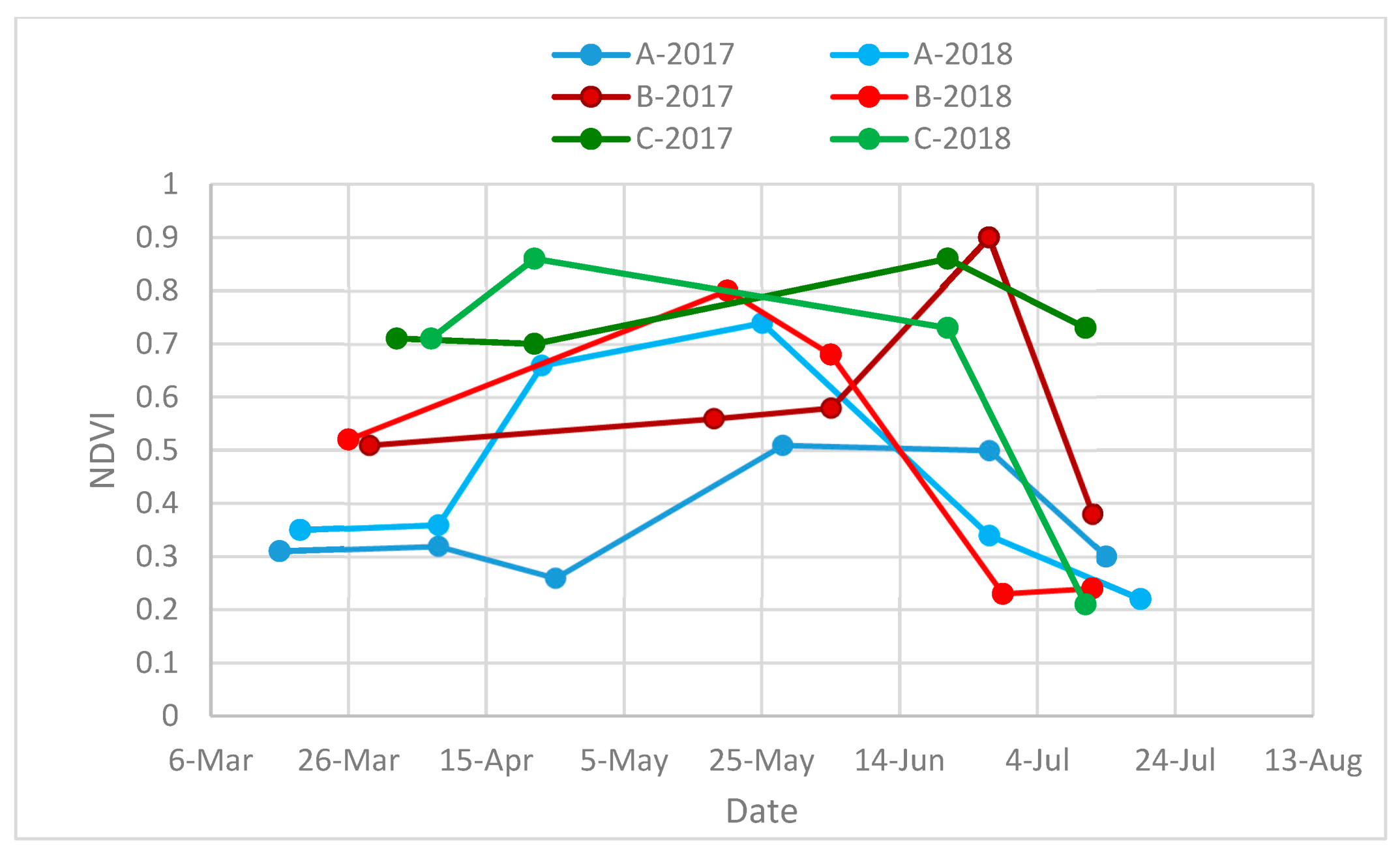
3.2. Changes in NDVI over the Vegetation Season and in Research Locations

Due to cloud cover, the availability of useful satellite images from Sentinel-2 was limited to 4–6 scenes per season during intensive growth of winter cereals, i.e., from half of March to half of July. Despite this limitation, it was possible to evaluate changes in VI values during the growing seasons. The most substantial differences between the average and a range of NDVI values for the three locations were observed from the end of March to the beginning of April. For location A, mean values of NDVI in both years were very low (0.3–0.4) until the beginning of April. The main cause of these low NDVI values in location A were lower air temperatures and consequently growing degree days (from sowing date to the end of April in 2017: location A—283, B—298, and C—451; in 2018: A—415; B—501, and C—605) during early spring than in the other two locations (Figure 2). The highest values of NDVI (of about 0.7 at the beginning of April) were observed in location C. This was caused by warmer conditions in both autumn and early spring as well as by more favorable soil conditions, which caused more intensive plant growth. The very high values of NDVI (0.7 or higher) in location C were observed for a much longer time, even until the end of June, in comparison to the other two locations. Consequently, this longer and more intensive crop growth in location C allowed us to obtain higher grain yields. In location B, NDVI values in early spring were at a medium level (higher than in location A and lower in comparison to location C) and very variable depending on the season at the later growth stages. In all locations, in 2017, a maximum NDVI value was achieved in very late June and much earlier in 2018, at the end of April (Figure 4, Table 4).

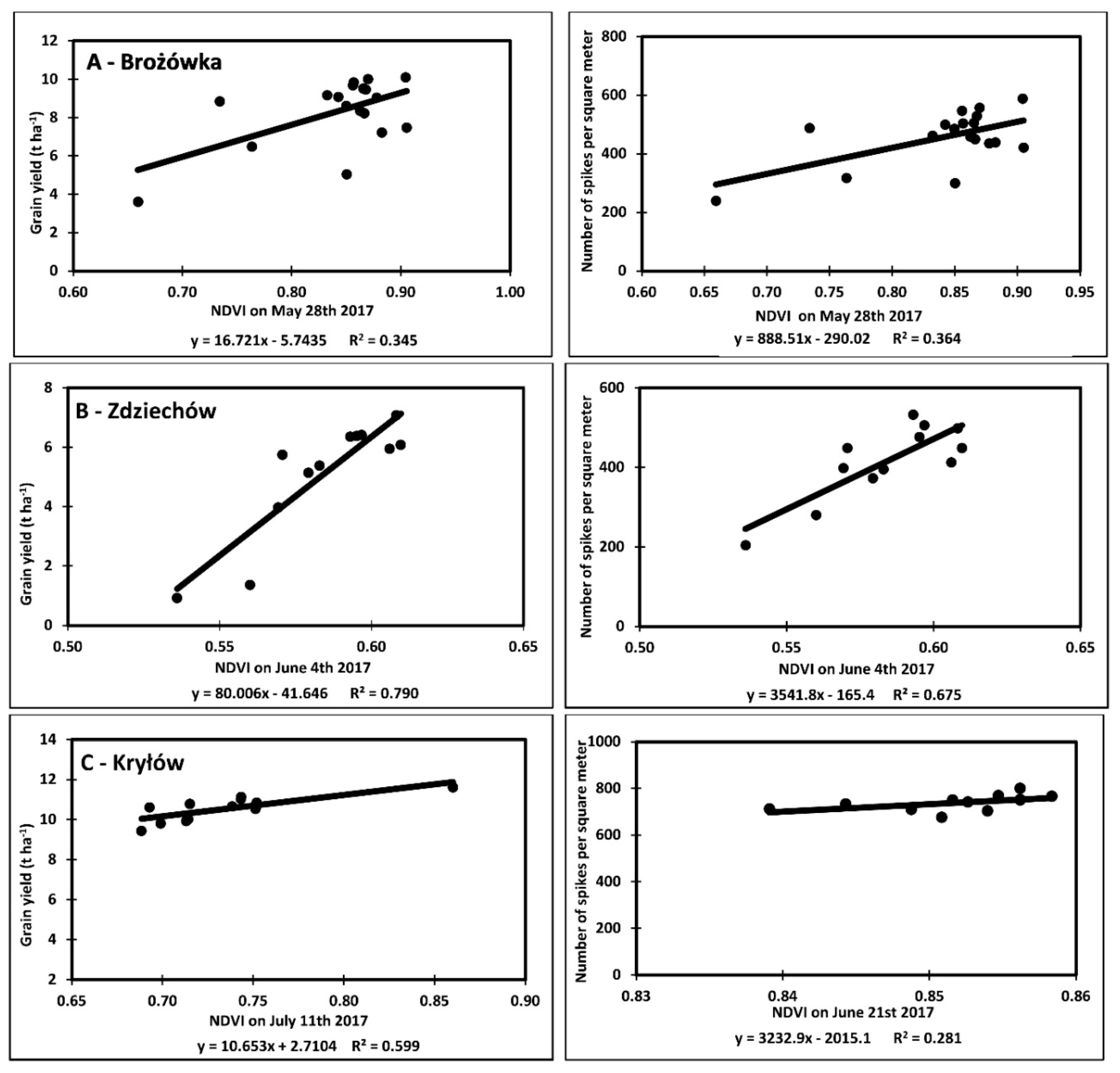
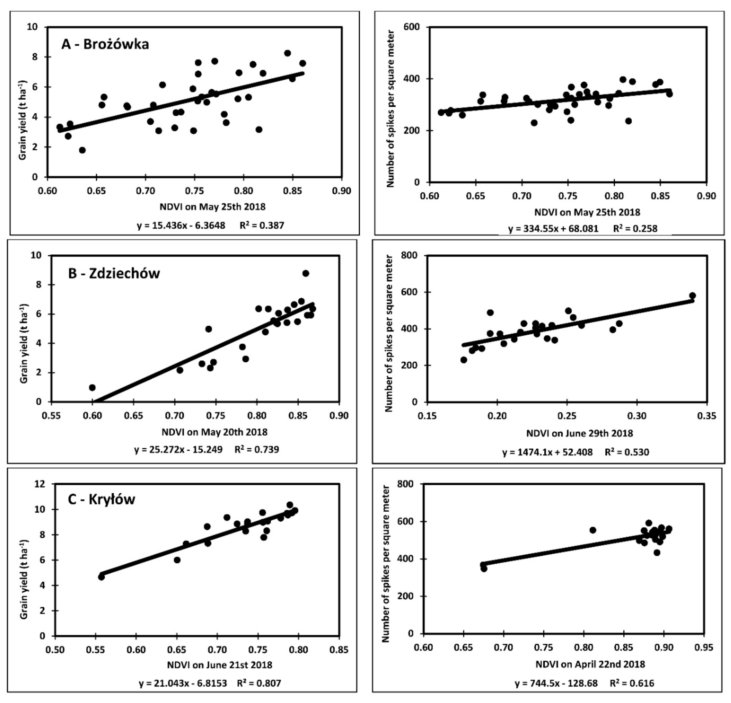
3.3. Relationships between NDVI and Grain Yield and Spike Number

One of the aims of the study was to determine the dates and plant growth stages when the relationships between VI values and grain yield, as well as number of spikes, were the strongest. The strongest correlations were achieved at various growth stages (Table 5 and Table 6).
For fields located in northeastern Poland, the highest correlation coefficients between grain yield and as well as number of spikes and NDVI were observed at the end of May (approximately shortly before or during the heading stage) in both years. On the basis of the regression slope values, it can be concluded that an increase in NDVI by 0.1 unit corresponded to the increase in grain yield by about 1.5–1.6 t∙ha−1 in both years (Figure 5 and Figure 6).
In location B, the strongest relationship between NDVI and grain yield was registered in late June of 2017 (end of milk maturity of winter wheat) and in the second half of May 2018 (shooting and heading of winter triticale). In this research site, the relationships were the strongest among the three examined locations, i.e., the R2 value was about 0.70–0.75 (Figure 6 and Figure 7). Moreover, the relationship between NDVI and the number of spikes was slightly weaker. The increase in NDVI by 0.1 unit was related to an increase in grain yield of about 8.0 t∙ha−1 in 2017 and about 2.5 t∙ha−1 in 2018.
In location C in 2017, the strongest correlation between NDVI and both grain yield and number of spikes was observed, respectively, on 21 June and 11 July (milk and dough maturity). In 2018, the strongest relationships between NDVI and both grain yield and spike number per square meter were obtained at the end of April and June. Due to a lack of data (clouds), it was not possible to verify this relationship at the end of May. The relationship was much stronger in 2018 than in 2017, mainly due to the considerably higher within-field variability of soil and consequently grain yield variability (Coefficient of Variation—CV) for grain yield was 6% and 16%, respectively, for 2017 and 2018). Based on the regression equations (Figure 5 and Figure 6), it was evaluated that an increase in NDVI by 0.1 unit was related to the increase in grain yield by about 1.0 t∙ha−1 in 2017 and about 2.1 t∙ha−1 in 2018. For all six site years, the strongest correlation between NDVI and grain yield and number of spikes was observed on similar dates and at similar growth stages. This is because the number of spikes per square meter usually very strongly affects grain yield.

3.4. Relationships between the Other Vegetation Indices and Grain Yield and Spike Number

Regression analyses performed to evaluate the strength of the relationship between the vegetation indices (SAVI, mSAVI, mSAVI2, GEMI, IPVI, RVI) and grain for each crop in 2017 and 2018 (Figure 7) indicated that the strongest relationships were observed for most of the VIs on the same dates. In location A, the highest correlations were observed at the end of May (end of shooting stage) in 2017, and from late May to mid-June (heading stage) in 2018. In location B, in 2017, the value of the correlation coefficients differed for individual VIs on several dates, while, in 2018, the strongest relationships were achieved in mid-May (beginning of heading stage) and at the end of June (milk maturity stage) for all VIs. The highest differentiation in the correlation coefficient values for the relationship between various VIs and yields was observed at the end of June and beginning of July (milk maturity stage) of 2017 in location C. In 2018, in all locations, the correlation coefficients had similar values for all VIs across the whole season.
The vegetation indices (VI) are ranked by order of decreasing correlation (data not shown) with yield as follows: SAVI, MSAVI, NDVI, MSAVI2, IPVI, RVI, GEMI. This ranking was carried out by averaging the R2 values from all of the measurement dates and research areas. The strength of the correlation of VIs with the number of ears was evaluated in the same way as above, and the order of decreasing correlation was as follows: NDVI, SAVI, MSAVI, MSAVI2, IPVI, RVI, GEMI.

4. Discussion

Constant field monitoring using RS methods is important not only for grain yield prediction, but also for the assessment of the site-specific conditions of plant development during the growing season [31,32]. This may allow us to introduce site-specific management of the field, and thus increase yields or save inputs.

4.1. Relationships between NDVI and Grain Yield

Our results for winter cereals, which constitute the majority of crop production in Central Europe, proved moderate and strong relationships (R2 in range of 0.35–0.81 for all fields in two seasons, Figure 5 and Figure 6) between the NDVI and grain yield of winter wheat and triticale for all of the studied fields. At location A, the correlation coefficient grew from mid-March to the end of May, when it reached the highest value. From the beginning of June to mid-July, we noticed a decrease in this correlation. The highest correlation coefficients are observed from the beginning of June to mid-July due to the growth stages such as heading, milk maturity, or dough maturity for location B. At the site C, we can see high rates of milk maturity at the end of June. A similar tendency, though with lower correlation values, can be observed when comparing the number of spikes per square meter. Similar results were achieved by Benedetti and Rossini (1993) [4] in Italy and by Smith et al. (1995) [5] in Western Australia for wheat. In both studies, AVHRR/NOAA satellite data were used for the calculation of NDVI. In Italy, R2 coefficient values for the relationship between NDVI and grain yield ranged from 0.24 to 0.749, and for Australia they ranged from 0.46 to 0.72. Ali et al. (2019) [17] observed higher R2 values of 0.878 and 0.926 for the relationship between the grain yield of winter and bread durum wheat and NDVI when the values of this index were derived from Landsat images. In turn, Labus et al. (2002) [6] achieved low R2 values ranging from 0.00 to 0.69 when wheat yield prediction was based on NDVI derived from AVHRR/NOAA satellite data. In our study, very low R2 values were obtained in April and May, and higher R2 values were mainly close to the heading stage and at the end of the growing season (Table 5 and Table 6). Therefore, while comparing many different studies, we can expect that, regardless of the research region, the relationship between NDVI and the grain yield remains at a similar level depending on the growth stage of the studied cereal.

4.2. Determination of Dates and Plant Growth Stages When Relationship between NDVI and Grain Yield Was the Strongest

Veloso et al. (2017) [10] found, for southeastern France, that NDVI reached maximum values in the second half of May, while, in Poland, depending on the research location, the highest NDVI values were reached from the end of April to the end of June (Figure 4). The site-related differences in the absolute NDVI values and the date at which they reached their maximum may primarily be influenced by the environmental conditions, mainly weather and soil conditions. This, in turn, closely depends on the climate in a specific region (amount of rainfall, growing degree days) and the amount of nitrogen applied. In the study of Naser et al. (2020) [33], much stronger correlations between NDVI, measured using a ground sensor, and the grain yield of winter wheat were observed for dryland than for irrigated conditions. The reason for such results was the greater range of absolute NDVI values for dryland in comparison to irrigated conditions. In that study, the highest correlations were observed after anthesis for both types of conditions. Very strong relationships between NDVI, measured using a ground spectrometer, and wheat yield were observed in a study where the effect of various nitrogen doses (from 0 to 210 kg/ha) was investigated [34]. The strongest correlations (R2 up to 0.96) were achieved at the heading stage. According to Satir and Berberoglu (2016) [35], the strength of the relationship between satellite-derived NDVI and the yields of wheat, corn and cotton was modified by soil conditions, e.g., soil salinity. This is because soil surface and soil water content can affect the values of vegetation indices, as well as the fact that water availability for plants is limited in high-salinity conditions. A better prediction of grain yield in the variable soil conditions of south Turkey can be achieved not only using prediction models such as NDVI, but also other spectral indices such as Normalized Difference Water Index (NDWI), Soil-Adjusted Vegetation Index (SAVI) or Tasseled Cap Wetness Index (WETNESS). The highest prediction accuracy for wheat was using the model which includes NDVI, NDWI and WETNESS. Prediction of wheat yield based on satellite-derived NDVI was improved if auxiliary data such as grain yield from previous seasons were included in models [36]. Dempewolf et al. (2013) [12] obtained the highest R2 values of 0.964 for NDVI and the yield of wheat grown in Pakistan six weeks before harvest. In our studies, the highest R2 value was observed at the end of April, i.e., about 12 weeks before harvest in the case of the field located in southeastern Poland. These results are similar to those of Kussul et al. [13] (2014), obtained in Ukraine, where a good prediction of winter wheat yields was possible even 2–3 months before harvest. The latest date (beginning of July) when the correlation coefficient for the relationship yield versus NDVI was the highest was observed in location B (Zdziechów) in central Poland in 2017. Similar results were obtained in Hungary by Nagy et al. (2018) [15] and Lopresti et al. (2015) [11] in Argentina, where good yield prediction was possible six weeks before harvest. Ali et al. (2019) [17] observed the highest correlation between NDVI and yield for winter bread wheat from stem elongation to the milk maturity of the grain, i.e., 6–17 weeks before harvest. In summary, the choice of the date of the yield estimation with the best accuracy does not depend only on long-term field and satellite measurements. Environmental, weather, and soil conditions should also be taken into account. As shown above, a yield estimation can be properly performed even between 3 months and 6 weeks before harvest, depending on the research region and the field-specific conditions.

4.3. Relationship between Other VIs and Grain Yield

According to Purevdorj et al. (1998) [37], SAVI and its modifications usually show higher correlations with grain at the beginning of the growing season compared to NDVI. According to Ren et al. (2018) [38], SAVI, with its modifications, should be used to estimate vegetation coverage at low vegetation density on arable land. In our study, the value of the correlation coefficient for the relationship between SAVI and grain yield was similar to the relationship with NDVI for both seasons and locations. Moreover, only in locations A and C in 2017 were the correlations between SAVI and grain yield stronger in early spring. For location A, during two vegetative seasons, we saw an increase in the correlation coefficient at the beginning of the growing season and a decrease in the cereals’ subsequent growth stages. For location B, the correlation coefficient increases until the beginning of June and slightly decreases until the end of July. In tested area C, an increase in the correlation coefficient value is noticed until mid-June, followed by a sharp decline by the end of July.
Ali et al. (2019) [17] selected NDVI and SR (referred to RVI in our study) as better VIs in comparison to EVI, SAVI, GNDVI, and GCI. Their conclusion was that SAVI never exhibited the strongest correlation with yield in comparison with other VIs, although, its correlation with grain yields was, most frequently, significant and strong. On the contrary, our research results proved that SAVI (and its modifications) and NDVI are ranked as VIs with the highest correlations with yield and number of spikes.
Moreover, Ali et al. (2019) [17] obtained R2 values of about 0.8 for durum and bread wheat yield and NDVI, EVI, and SR. We achieved Pearson’s correlation values of 0.4 between winter wheat and triticale yield and SAVI, but 0.3 with mSAVI, NDVI, IPVI, RVI (SR), and GEMI. These differences most probably arise from a different method being used for the collection of yield data.

5. Conclusions

Various vegetation indices (SAVI, MSAVI, NDVI, MSAVI2, IPVI, RVI and GEMI), their calculation based on the red and near-infrared radiation derived from the Sentinel−2 imagery, showed similar relationships with grain yield and number of spikes per square meter of winter wheat and triticale as the commonly used NDVI. While comparing the grain yield and the number of spikes from NDVI for all three locations during two seasons, it can be seen that the values of R2 for the number of spikes per square meter are lower than the values of R2 for the grain yield. Consequently, the grain yield is a better yield prediction parameter than number of spikes per square meter. In general, the relationship between NDVI values and grain yield was stronger at more advanced growth stages. Depending on the region of Poland, the strongest correlations between NDVI and yield and its main component were obtained for NDVI derived from images obtained at the end of April (beginning of shooting) in southeastern Poland, at the end of May (beginning of heading) in the northeastern part of the country and only at the end of June (at milk maturity) in the central region of Poland. The divergence in these periods may result from the sowing date, but also from different climatic conditions, especially GDD values, in the three micro-climate regions of Poland. The different strengths of the relationships may be caused by the soil water deficiency due to variable weather and soil conditions, depending on the research location, at different growth stages. Within-field water variability was higher, especially on sandy soils (which were common in some parts of the field in location B) at later growth stages when air temperatures were higher and negative balance between rainfall and evapotranspiration was more common than in locations A and C [39]. Moreover, the presence of clouds, which made the registration of useful satellite images impossible on some dates, also contributed to the results obtained in this study. For example, in location C in southeastern Poland, there were no cloudless images available in May in both seasons and, because of this, it was not possible to evaluate the relationships between VIs and yield for some important growth stages of the crop. The proposed estimated time for accurate yield prediction is about 4–6 weeks before harvest (from the beginning of shooting to milk maturity).

Author Contributions

Conceptualization, E.P., D.G.; methodology, E.P., D.G., M.S., formal analysis, E.P., D.G., M.S.; investigation, E.P., D.G., M.S., S.S.; data curation, E.P., D.G.; writing—original draft preparation, E.P., D.G., M.S., S.S.; writing—review and editing, E.P., D.G., M.S., D.R., B.B., S.S.; visualization, E.P., D.G.; supervision, D.G.; project administration, D.R., B.B.; funding acquisition, D.R., B.B. All authors have read and agreed to the published version of the manuscript.

Funding

This research was funded by the European Space Agency, FERTISAT—Satellite-based Service for Variable Rate Nitrogen Application in Cereal Production, grant number 4000118613/16/NL/EM.

Conflicts of Interest

The authors declare no conflict of interest.

References

  1. Szantoi, Z.; Strobl, P. Copernicus Sentinel-2 Calibration and Validation. Eur. J. Remote Sens. 2019, 52, 253–255. [Google Scholar] [CrossRef] [Green Version]
  2. Sentinel-2 User Handbook-Document Library-Sentinel Online. Available online: https://sentinels.copernicus.eu/web/sentinel/user-guides/document-library/-/asset_publisher/xlslt4309D5h/content/sentinel-2-user-handbook (accessed on 17 August 2020).
  3. Asrar, G.; Fuchs, M.; Kanemasu, E.T.; Hatfield, J.L. Estimating absorbed photosynthetic radiation and Leaf Area Index from spectral reflectance in wheat. Agron. J. 1984, 76, 300–306. [Google Scholar] [CrossRef]
  4. Benedetti, R.; Rossini, P. On the use of NDVI profiles as a tool for agricultural statistics: The case study of wheat yield estimate and forecast in Emilia Romagna. Remote Sens. Environ. 1993, 45, 311–326. [Google Scholar] [CrossRef]
  5. Smith, R.C.G. Forecasting wheat yield in a Mediterranean-type environment from the NOAA satellite. Aust. J. Agric. Res. 1995, 46, 113–125. [Google Scholar]
  6. Labus, M.P.; Nielsen, G.A.; Lawrence, R.L.; Engel, R.; Long, D.S. Wheat yield estimates using multi-temporal NDVI satellite imagery. Int. J. Remote Sens. 2002, 23, 4169–4180. [Google Scholar] [CrossRef]
  7. Shou, L.; Jia, L.; Cui, Z.; Chen, X.; Zhang, F. Using high-resolution satellite imaging to evaluate nitrogen status of winter wheat. J. Plant Nutr. 2007, 30, 1669–1680. [Google Scholar] [CrossRef]
  8. Jeppesen, J.H.; Jacobsen, R.H.; Jørgensen, R.N.; Halberg, A.; Toftegaard, T.S. Identification of high-variation fields based on open satellite imagery. Adv. Anim. Biosci. 2017, 8, 388–393. [Google Scholar] [CrossRef] [Green Version]
  9. Delegido, J.; Verrelst, J.; Alonso, L.; Moreno, J. Evaluation of Sentinel-2 red-edge bands for empirical estimation of green LAI and chlorophyll content. Sensors 2011, 11, 7063–7081. [Google Scholar] [CrossRef] [Green Version]
  10. Veloso, A.; Mermoz, S.; Bouvet, A.; Le Toan, T.; Planells, M.; Dejoux, J.F.; Ceschia, E. Understanding the temporal behavior of crops using Sentinel-1 and Sentinel-2-like data for agricultural applications. Remote Sens. Environ. 2017, 199, 415–426. [Google Scholar] [CrossRef]
  11. Lopresti, M.F.; Di Bella, C.M.; Degioanni, A.J. Relationship between MODIS-NDVI data and wheat yield: A case study in Northern Buenos Aires province, Argentina. Inf. Process. Agric. 2015, 2, 73–84. [Google Scholar] [CrossRef] [Green Version]
  12. Dempewolf, J.; Adusei, B.; Becker-Reshef, I.; Barker, B.; Potapov, P.; Hansen, M.; Justice, C. Wheat Production Forecasting for Pakistan from Satellite Data. In 2013 IEEE International Geoscience and Remote Sensing Symposium-IGARSS; IEEE: Melbourne, Australia, 2013; pp. 3239–3242. [Google Scholar]
  13. Kussul, N.; Kolotii, A.; Skakun, S.; Shelestov, A.; Kussul, O.; Oliynuk, T. Efficiency Estimation of Different Satellite Data Usage for Winter Wheat Yield Forecasting in Ukraine. In 2014 IEEE Geoscience and Remote Sensing Symposium; IEEE: Quebec City, QC, Canada, 2014; pp. 5080–5082. [Google Scholar]
  14. Bu, H.; Sharma, L.K.; Denton, A.; Franzen, D.W. Comparison of satellite imagery and ground-based active optical sensors as yield predictors in sugar beet, spring wheat, corn, and sunflower. Agron. J. 2017, 109, 299–308. [Google Scholar] [CrossRef] [Green Version]
  15. Nagy, A.; Fehér, J.; Tamás, J. Wheat and maize yield forecasting for the Tisza river catchment using MODIS NDVI time series and reported crop statistics. Comput. Electron. Agric. 2018, 151, 41–49. [Google Scholar] [CrossRef]
  16. Yang, A.; Zhong, B.; Wu, J. Monitoring Winter Wheat in ShanDong Province Using Sentinel Data and Google Earth Engine Platform. In 2019 10th International Workshop on the Analysis of Multitemporal Remote Sensing Images; IEEE: Shanghai, China, 2019; pp. 1–4. [Google Scholar]
  17. Ali, A.; Martelli, R.; Lupia, F.; Barbanti, L. Assessing multiple years’ spatial variability of crop yields using satellite vegetation indices. Remote Sens. 2019, 11, 2384. [Google Scholar] [CrossRef] [Green Version]
  18. GUS Statistical Yearbook of Agriculture. 2019. Available online: https://stat.gov.pl/en/topics/statistical-yearbooks/statistical-yearbooks/statistical-yearbook-of-agriculture-2019,6,14.html (accessed on 16 August 2020).
  19. Kottek, M.; Grieser, J.; Beck, C.; Rudolf, B.; Rubel, F. World Map of the Köppen-Geiger climate classification updated. Meteorol. Z. 2006, 15, 259–263. [Google Scholar] [CrossRef]
  20. Open Access Hub. Available online: https://scihub.copernicus.eu/ (accessed on 16 August 2020).
  21. Brief Introduction to Remote Sensing—Semi-Automatic Classification Plugin 6.4.0.2-Documentation. Available online: https://semiautomaticclassificationmanual.readthedocs.io/pl/latest/remote_sensing.html#dos1-correction. (accessed on 16 August 2020).
  22. Rouse, J.W., Jr.; Haas, R.H.; Deering, D.W.; Schell, J.A.; Harlan, J.C. Monitoring the vernal advancement and retrogradation (Green Wave Effect) of natural vegetation. In Great Plains Corridor; Final Rep. RSC 1978–4; Remote Sensing Center, Texas A&M Univ.: College Station, TX, USA, 1974. [Google Scholar]
  23. Wang, J.; Rich, P.M.; Price, K.P.; Kettle, W.D. Relations between NDVI and tree productivity in the central Great Plains. Int. J. Remote Sens. 2004, 25, 3127–3138. [Google Scholar] [CrossRef]
  24. Huete, A.R. A soil-adjusted vegetation index (SAVI). Remote Sens. Environ. 1988, 25, 295–309. [Google Scholar] [CrossRef]
  25. Jiang, Z. Interpretation of the modified soil-adjusted vegetation index isolines in red-NIR reflectance space. J. Appl. Remote Sens. 2007, 1, 013503. [Google Scholar] [CrossRef] [Green Version]
  26. Crippen, R. Calculating the vegetation index faster. Remote Sens. Environ. 1990, 34, 71–73. [Google Scholar] [CrossRef]
  27. Pinty, B.; Verstraete, M.M. GEMI: A non-linear index to monitor global vegetation from satellites. Vegetatio 1992, 101, 15–20. [Google Scholar] [CrossRef]
  28. Jordan, C.F. Derivation of Leaf-Area Index from quality of light on the forest floor. Ecology 1969, 50, 663–666. [Google Scholar] [CrossRef]
  29. Orfeo ToolBox 7.1.0 Documentation. Available online: https://www.orfeo-toolbox.org/CookBook/ (accessed on 17 August 2020).
  30. Welcome to the QGIS Project! Available online: https://www.qgis.org/en/site/ (accessed on 16 August 2020).
  31. Mengmeng, D.; Noboru, N.; Atsushi, I.; Yukinori, S. Japan multi-temporal monitoring of wheat growth by using images from satellite and unmanned aerial vehicle. Int. J. Agric. Biol. Eng. 2017, 10, 1–13. [Google Scholar] [CrossRef]
  32. Toscano, P.; Castrignanò, A.; Di Gennaro, S.F.; Vonella, A.V.; Ventrella, D.; Matese, A.A. Precision agriculture approach for durum wheat yield assessment using remote sensing data and yield mapping. Agronomy 2019, 9, 437. [Google Scholar] [CrossRef] [Green Version]
  33. Naser, M.A.; Khosla, R.; Longchamps, L.; Dahal, S. Using NDVI to differentiate wheat genotypes productivity under dryland and irrigated conditions. Remote Sens. 2020, 12, 824. [Google Scholar] [CrossRef] [Green Version]
  34. Chandel, N.S.; Tiwari, P.S.; Singh, K.P.; Jat, D.; Gaikwad, B.B.; Tripathi, H.; Golhani, K. Yield prediction in wheat (Triticum aestivum L.) using spectral reflectance indices. Curr. Sci. 2019, 116, 272. [Google Scholar] [CrossRef]
  35. Satir, O.; Berberoglu, S. Crop yield prediction under soil salinity using satellite derived vegetation indices. Field Crops Resolut. 2016, 192, 134–143. [Google Scholar] [CrossRef]
  36. Fieuzal, R.; Bustillo, V.; Collado, D.; Dedieu, G. Combined use of multi-temporal Landsat-8 and Sentinel-2 images for wheat yield estimates at the intra-plot spatial scale. Agronomy 2020, 10, 327. [Google Scholar] [CrossRef] [Green Version]
  37. Purevdorj, T.S.; Tateishi, R.; Ishiyama, T.; Honda, Y. Relationships between percent vegetation cover and vegetation indices. Int. J. Remote Sens. 1998, 19, 3519–3535. [Google Scholar] [CrossRef]
  38. Ren, H.; Zhou, G.; Zhang, F. Using negative soil adjustment factor in soil-adjusted vegetation index (SAVI) for aboveground living biomass estimation in arid grasslands. Remote Sens. Environ. 2018, 209, 439–445. [Google Scholar] [CrossRef]
  39. The Agricultural Drought Monitoring System. Available online: http://susza.iung.pl/en/ (accessed on 16 August 2020).
Figure 1. Location of the three research sites in Poland (Open Geospatial Consortium (OGC) Web Map Service).
Agronomy 10 01842 g001
Figure 2. Monthly sums of precipitation, mean air temperature and growing degree days (GDD) for meteorological stations located closest to the research sites (for location A—Olecko, for location B—Puławy, for location C—Strzyżów) from the IMGW-PIB national institute (source of data: https://danepubliczne.imgw.pl/).
Agronomy 10 01842 g002
Figure 3. Normalized Difference Vegetation Index (NDVI) maps of the experimental fields in three locations ((a,b): Brożówka—A, (c,d): Zdziechów—B, and (e,f): Kryłów—C) in two seasons: 2017 (on the left) and 2018 (on the right), from dates when maximum average value of this index was achieved, with soil and plant sampling points superimposed. Explanation of color representation of NDVI values and the dates of NDVI acquisition are given.
Agronomy 10 01842 g003
Figure 4. Mean values of NDVI values for six fields (three locations: A—Brożówka, B—Zdziechów, and C—Kryłów in two years: 2017 and 2018).
Agronomy 10 01842 g004
Figure 5. Relationships between grain yield (charts in the left side), number of spikes per square meter (charts in the right side) and NDVI values for three locations (A—Brożówka, B—Zdziechów, C—Kryłów) for the dates when the correlations reached maximum values in 2017. Regression equations and the value of the R2 coefficient are given for each relationship.
Agronomy 10 01842 g005
Figure 6. Relationships between grain yield (charts in the left side), number of spikes per square meter (charts in the right side) versus NDVI for three locations (A—Brożówka, B—Zdziechów, C—Kryłów) for the date when their correlations reached maximum values in 2018. Regression equations and the value of the R2 coefficient are given for each relationship.
Agronomy 10 01842 g006
Figure 7. Values of correlation coefficients between vegetation indices and grain yield (t∙ha−1) in three locations (A—Brożówka, B—Zdziechów, C—Kryłów) on the selected dates in years 2017 (charts in the left side) and 2018 (charts in the right side).
Agronomy 10 01842 g007
Table 1. Characteristics of the studied fields in three locations and in two years.
Location A—BrożówkaLocation B—ZdziechówLocation C—Kryłów
Year201720182017201820172018
Cropwinter wheatwinter triticalewinter wheatwinter triticalewinter wheatwinter wheat
Sowing date20 September 201627 September 201727 September 201628 September 201722 September 201623 September 2017
Area of the field (ha)14.914.99.77.89.79.6
Geographical coordinates54°6′36″ N,
22°0′3.6″ E
54°6′36″ N,
22°0′3.6″ E
51°24′57.6″ N,
21°3′7.2″ E
51°25′1.2″ N,
21°3′10.8″ E
50°41′27.6″ N, 24°1′58.8″ E50°42′32.4″ N, 24°3′10.8″ E
Soil WRB 2015 Reference Group-dominant (associated) *Luvisols (Phaeozems, Histosols, Gleysols, Cambisols, Regosols)Luvisols (Phaeozems, Histosols, Gelysols, Cambisols, Regosols)Phaeozems (Luvisols, Arenosols)Luvisols (Arenosols)GleysolsLuvisols
USDA soil texture class dominant (associated) *sandy loam (loam, clay loam)sandy loam (loam, clay loam)sandy loam (loam, clay loam, loamy sand, sand)loamy sand (sandy loam, sand)silt loam (silty clay loam, silty clay)silt loam (silty clay loam)
Number of sampling points of soil in spring/plots used at harvest for grain yield and spike number evaluation16/1818/3610/1212/2410/1212/21
Available elements in soil in a layer of 0–30 cm (mg∙kg−1) ***P71.5 (92.0) **52.2 (18.4)55.4 (16.6)118.0 (42.8)119.5 (31.8)79.8 (41.8)
K160.2 (104.6)143.6 (44.6)112.1 (27.4)106.8 (19.4)175.1 (32.4)193.7 (38.6)
Mg109.7 (206.2)150.8 (135.0)67.5 (32.0)69.7 (47.3)54.9 (13.3)78.8 (22.1)
pH6.2 (0.8)6.5 (0.7)5.7 (0.5)5.8 (0.5)6.0 (0.4)6.7 (0.3)
* Approximated soil data based on early spring field examination obtained during soil augerings done in locations of spike sampling (see Figure 3). **—means and standard deviations in parentheses. ***—using Mehlich 3 extract.
Table 2. Dates for which satellite-based vegetation indices were derived from Sentinel images for three locations and two seasons.
Location A BrożówkaLocation B ZdziechówLocation C Kryłów
201720182017201820172018
16 March19 March29 March26 March2 April7 April
8 April8 April18 May20 May22 April22 April
25 April23 April4 June4 June21 June21 June
28 May25 May27 June29 June11 July11 July
27 June27 June12 July12 July--
14 July19 July----
Table 3. Grain yield (t ha−1) and number of spikes per m2 m in sampling points at harvest in Brożówka (A), Zdziechów (B), and Kryłów (C) in 2017 and 2018.
Grain Yield (t ha−1)Spikes Number Per m2
Location and YearMeanSDCVMin.Max.MeanSDCVMin.Max.
A 20178.331.7721.2%3.6210.145891.520.0%240589
A 20185.101.6332.0%1.808.2631743.313.7%230397
B 20175.071.9939.3%0.937.0841595.423.0%205533
B 20185.011.8637.1%0.988.7938977.519.9%231582
C 201710.50.636.0%9.4311.673934.04.6%676801
C 20188.631.3816.0%4.6710.451462.012.1%348593
Table 4. Mean values and ±SD of vegetation indices for the dates when the highest NDVI values were observed.
Location and DateNDVISAVImSAVImSAVI2IPVIGEMIRVI
A 28 May 20170.84 ± 0.060.51 ± 0.050.51 ± 0.050.59 ± 0.070.92 ± 0.030.83 ± 0.0412.95 ± 3.93
A 25 May 20180.74 ± 0.070.49 ± 0.050.44 ± 0.050.49 ± 0.070.87 ± 0.030.78 ± 0.047.31 ± 2.25
B 27 June 20170.90 ± 0.010.42 ± 0.030.65 ± 0.030.35 ± 0.030.39 ± 0.049.38 ± 1.300.80 ± 0.03
B 20 May 20180.80 ± 0.060.52 ± 0.060.47 ± 0.070.53 ± 0.080.90 ± 0.030.80 ± 0.069.88 ± 2.78
C 21 June 20170.86 ± 0.020.62 ± 0.080.57 ± 0.090.63 ± 0.010.90 ± 0.080.85 ± 0.0911.52 ± 3.39
C 22 April 20180.86 ± 0.070.60 ± 0.060.55 ± 0.070.64 ± 0.090.93 ± 0.030.87 ± 0.0515.39 ± 3.99
Table 5. Correlation coefficients (r) between NDVI values and grain yield (t∙ha−1) for three locations in 2017 and 2018. The background color of the cells with the correlation coefficient values indicates the strength of the relationship (significant correlations at α = 0.05 are given in bold).
LocationDate (2017)Growth Stage *rLocationDate (2018)Growth Stager
A16-Marchtillering0.421A19-Marchtillering0.254
8-Apriltillering0.4938-Apriltillering0.241
25-Apriltillering/shooting0.34123-Apriltillering/shooting0.389
28-Mayshooting/heading0.58725-Mayshooting/heading0.622
27-Junemilk maturity0.44127-Junemilk maturity0.570
14-Julydough maturity0.23919-Julydough maturity−0.012
B29-Marchtillering−0.457B26-Marchtillering0.064
18-Mayshooting/heading0.15420-Mayshooting/heading0.859
4-Juneheading/flowering0.8894-Juneheading/flowering0.790
27-Junemilk maturity0.84029-Junemilk maturity0.804
12-Julydough maturity0.69312-Julydough maturity−0.152
C2-Apriltillering−0.423C7-Apriltillering0.713
22-Apriltillering/shooting0.06722-Apriltillering/shooting0.795
21-Junemilk maturity0.59421-Junemilk maturity0.899
11-Julydough maturity0.77411-Julydough maturity0.361
−1.0−0.9−0.8−0.7−0.6−0.5−0.4−0.3−0.2−0.10.10.20.30.40.50.60.70.80.91.0
very strong negative correlationvery strong positive correlation
*—approximated growth stages of the whole field crop.
Table 6. Correlation coefficients (r) between NDVI values and number of spikes per square meter for three locations in 2017 and 2018. The background color of the cells with the correlation coefficient values indicates the strength of the relationship (significant correlations at α = 0.05 are given in bold).
LocationDate (2017)Growth Stage *rLocationDate (2018)Growth Stager
A16-Marchtillering0.452A19-Marchtillering0.102
8-Apriltillering0.5358-Apriltillering0.120
25-Apriltillering/shooting0.37223-Apriltillering/shooting0.167
28-Mayshooting/heading0.60325-Mayshooting/heading0.508
27-Junemilk maturity0.47127-Junemilk maturity0.485
14-Julydough maturity0.28819-Julydough maturity−0.096
B29-Marchtillering−0.341B26-Marchtillering0.068
18-Mayshooting/heading0.15920-Mayshooting/heading0.685
4-Juneheading/flowering0.8224-Juneheading/flowering0.625
27-Junemilk maturity0.78629-Junemilk maturity0.728
12-Julydough maturity0.52912-Julydough maturity−0.064
C2-Apriltillering0.025C7-Apriltillering0.731
22-Apriltillering/shooting−0.16222-Apriltillering/shooting0.785
21-Junemilk maturity0.64921-Junemilk maturity0.647
11-Julydough maturity0.59211-Julydough maturity0.275
−1.0−0.9−0.8−0.7−0.6−0.5−0.4−0.3−0.2−0.10.10.20.30.40.50.60.70.80.91.0
very strong negative correlationvery strong positive correlation
*—approximated growth stages of the whole field crop.
Publisher’s Note: MDPI stays neutral with regard to jurisdictional claims in published maps and institutional affiliations.

