Article

A Remote Sensing-Based Approach to Management Zone Delineation in Small Scale Farming Systems

1
James Hutton Institute, Errol Road, Invergowrie DD25BQ, UK
2
College of Resource and Environmental Sciences, China Agricultural University, 2 Yuanmingyuan W. Rd, Beijing 100193, China
3
RSK ADAS Ltd., 172 Chester Road, Helsby WA60AR, UK
4
Department of Biosystems Engineering, Auburn University, 200 Tom Corley Building, Auburn, AL 36849, USA
5
Precision Agriculture Center, Department of Soil, Water and Climate, University of Minnesota, 1991 Upper Buford Circle, St. Paul, MN 55108, USA
*
Authors to whom correspondence should be addressed.
Current address: Department of Agronomy, Purdue University, West Lafayette, IN 47906, USA.
Agronomy 2020, 10(11), 1767; https://doi.org/10.3390/agronomy10111767
Submission received: 18 September 2020 / Revised: 6 November 2020 / Accepted: 7 November 2020 / Published: 12 November 2020
(This article belongs to the Special Issue Site-Specific Nutrient Management)

Abstract

:
Small-scale farms represent about 80% of the farming area of China, in a context where they need to produce economic and environmentally sustainable food. The objective of this work was to define management zone (MZs) for a village by comparing the use of crop yield proxies derived from historical satellite images with soil information derived from remote sensing, and the integration of these two data sources. The village chosen for the study was Wangzhuang village in Quzhou County in the North China Plain (NCP) (30°51′55″ N; 115°02′06″ E). The village was comprised of 540 fields covering approximately 177 ha. The subdivision of the village into three or four zones was considered to be the most practical for the NCP villages because it is easier to manage many fields within a few zones rather than individually in situations where low mechanization is the norm. Management zones defined using Landsat satellite data for estimation of the Green Normalized Vegetation Index (GNDVI) was a reasonable predictor (up to 45%) of measured variation in soil nitrogen (N) and organic carbon (OC). The approach used in this study works reasonably well with minimum data but, in order to improve crop management (e.g., sowing dates, fertilization), a simple decision support system (DSS) should be developed in order to integrate MZs and agronomic prescriptions.

1. Introduction

Small scale farms represent about 80% of the farming area of China. Given the need to produce more food on the same amount (or less) of land while also reducing environmental pollution, such areas are faced with tough challenges. Farmers manage their fields by experience and need science-based evidence to make the system more efficient. The mismanagement of nitrogen (N) fertilizer is a known problem in the smallholder farming systems of China [1].
Precision nutrient management can be achieved either through a sensor-based or a map-based approach. The former uses sensors to guide site-specific N management based on the quantification of crop reflectance. However, a sensor-based approach is affected by the inter-annual interactions between soil and weather. Colaço & Bramley [2] demonstrated how the sensor-based approach could be improved by also considering the impact of other environmental covariates. The latter approach consists of using multiple images (e.g., soil, remote sensing, yield monitor) with the aim of dividing the fields into management zones (MZs). MZs are defined as sub-regions within the field that have similar combinations of yield-limiting factors and are managed accordingly [3,4]. Basso et al. [5] stated that understanding the factors that lead to the spatial and temporal variability of a crop within the field is the first step for optimal agronomic management. In addition, the delineation of fields into MZs helps with obtaining soil/crop samples cost-effectively and applying site-specific agronomic input [4,5,6,7].
Several approaches have been proposed to define MZs at the field level. One approach is based on gathering soil or landscape information, such as sampling the soil using electrical conductivity (EC) sensor, sampling for soil physical and chemical properties or using remotely sensed data for estimating soil and landscape properties [8,9,10,11,12]. Another approach uses yield maps or remotely sensed images to reconstruct spatial and temporal patterns of crop growth within the field to define a given number of MZs [13,14,15,16]. Finally, the integrated approach uses both soil-landscape and crop information to define MZs at field level [4,17].
However, the small size of single farms in the North China Plain (NCP) does not allow for cost-effective on-farm management using farm-scale MZs. Moreover, yield maps are not available in most small-scale farming systems and, in such systems, farmers do not measure field-level yield at harvest [18], but measure total grain that they sell from all of their fields. Jin et al. [19] combined a crop simulation model with remotely sensed data to map yield heterogeneity on smallholder farms in East Africa. High-resolution satellite images were used to define a smallholder farming system, but the prevalence of small field size was one of the challenges in improving the performance of the approach proposed [19]. In addition, high-resolution satellite data usually has to be purchased from a private provider (e.g., RapidEye) or obtained from a contemporary open-source sensor such as Sentinel-2, which does not yet have enough years available to capture the long-term inter-annual variability. A practical strategy is to divide fields in a village into several MZs disregarding the current field management structure. Some of the common open-source satellites, such as Landsat that has a long time-series of data, may allow the mapping of fields in a village for MZ delineation purposes; therefore, each field can be classified in a given MZ, maintaining the existing boundary structure. Fields in the same MZ could then use similar management practices or inputs optimised for their particular conditions and requirements regardless of their geographical proximity.
The objective of this work was to integrate soil information derived from remote sensing with crop yield proxies derived from historical satellite images to define MZs at the village scale.

2. Materials and Methods

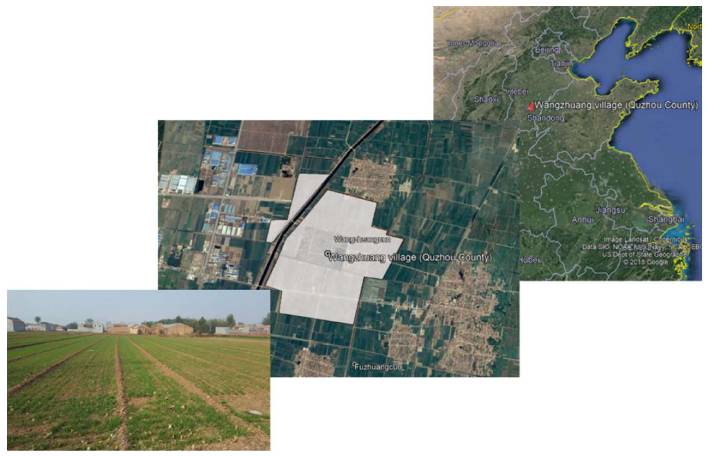
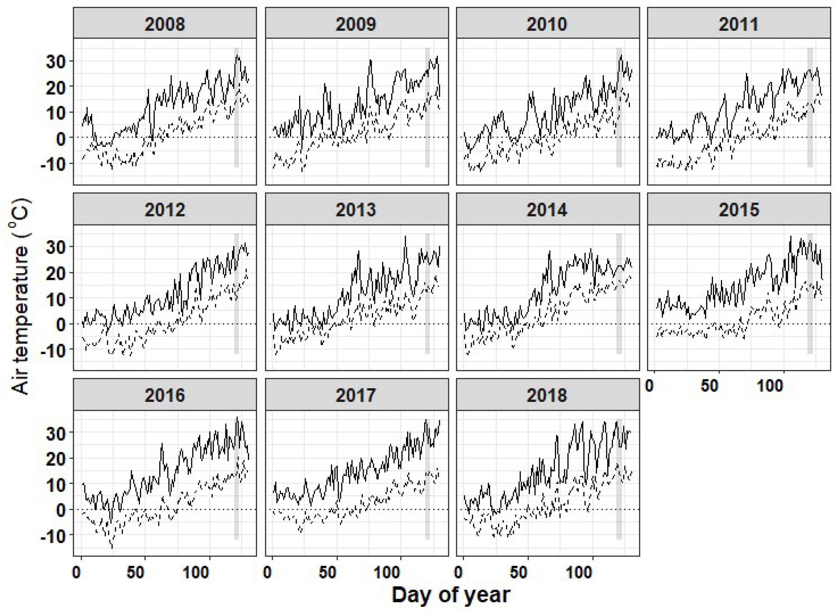
2.1. Site Description

The village chosen for the study was Wangzhuang village in Quzhou County in the NCP (36°51′55″ N; 115°02′06″ E). The cropped area of the village covered approximately 177 ha and comprised a total of 540 fields, with an average farm size of 0.33 ha (Figure 1). The village is part of the Science and Technology Backyards (STB) initiative. The STB was established originally in Quzhou County in 2009 by China Agricultural University to carry out specific research and extension services aimed at transferring research technology to smallholder farmers [18]. The main cropping system of the village was winter wheat (Triticum aestivum L.) (sown in October) and summer maize (Zea mays L.) (sown in mid-June), with irrigation used by farmers on both crops. The soil was classified as silty-loam [20] and no significant slopes were present. The 2008–2018 weather had a mean, maximum and minimum air temperature during the growing season of 9.7, 15, and 4.3 °C, respectively.

2.2. Overall Methodological Approach
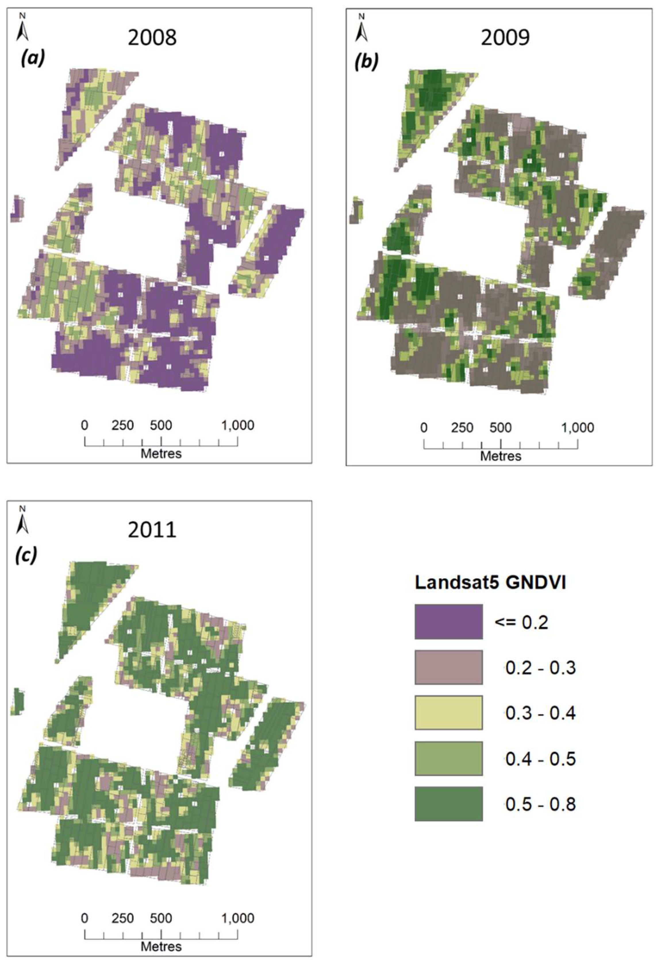
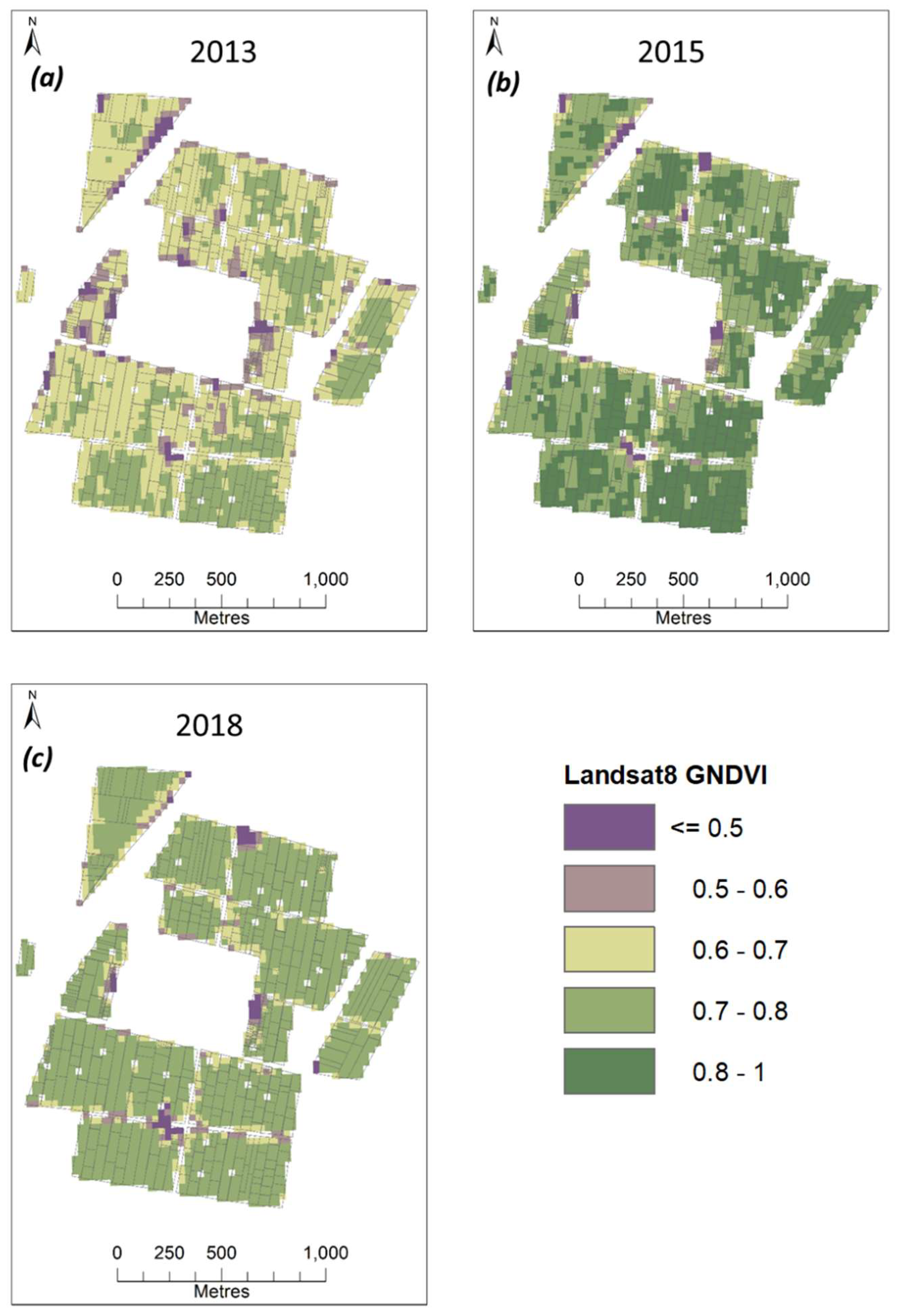
Satellite data for the village were obtained from the Landsat satellites (30 m pixels) for 2008–2018 using the USGS explorer website [21]. Level 2 processed imagery was requested and analyzed following the protocols described on the Landsat Explorer [21]. The Landsat data came from 2 different sensors having a different wavelength range in the near-infrared bands; one was used from 2008 to 2011 (Landsat 5 with 0.76–0.90 µm with Landsat Thematic Mapper - TM sensor [21]) and another from 2013 to 2018 (Landsat 8 with 0.85–0.88 µm with Operational Land Imager - OLI sensor [21]). Atmospherically-corrected cloud-free scenes from the end of April/beginning of May were selected to coincide with flowering in winter wheat. The choice of using images at that particular developmental stage was justified by the strong correlation between remote sensing data and grain yield [22,23,24]. In addition, in Northern China, the use of proximal and/or remote sensing as a proxy of canopy N and yield has been validated on several crops and in different geographical regions [25,26,27,28]. The Green Normalized Difference Vegetation Index (GNDVI) [29] was calculated for each scene. The GNDVI is more closely related to the photosynthetically absorbed radiation than NDVI and has shown a linear correlation with the Leaf Area Index (LAI) and biomass [29]. This makes the GNDVI more sensitive to changes in biomass and chlorophyll concentration compared to the NDVI. It was calculated as follows:
G N D V I =   ρ N I R ρ G r e e n ρ N I R + ρ G r e e n
where ρ N I R and ρ G r e e n are the reflectance in the Near Infrared and Green bands, respectively.
Soil Brightness (SOB) data at 3 m spatial resolution were purchased from Courtyard Agriculture Ltd. in the UK and were derived from RapidEye optical satellite images at a time in the season when the land was un-cropped (bare soil). Most of the fields were contiguous, with ‘boundaries’ being narrow ridges of bare soil. There was little other vegetation or paths/roads present. Therefore, most of the pixels corresponded to cropland (Figure 1).
Prior to sowing of wheat in 2015, soil sampling was carried out in the village. For each field, 10 samples were collected at 0–20 cm depth following “S” patterns. The samples were pooled together, mixed thoroughly and divided into four subsamples. One subsample of about 1–2 kg was kept for determining inorganic soil N and soil organic carbon (OC). The soil samples were later dried, ground to powder and analyzed for total soil N concentration using the Kjeldahl digestion method [30]. Soil OC was analyzed following the wet combustion method [31]. Soil texture information was also available at selected points and used for this study and additional information is available elsewhere [32].
Spatial and temporal variability in GNDVI were quantified following the method of Basso et al. (2012). The spatial variability of GNDVI from 2008 to 2018 was calculated from the relative percentage difference of GNDVI at each 30 m pixel from the average GNDVI obtained for the whole cropped area of the village, according to Equation (2) [13]:
σ ¯ s i 2 =   1 n k = 1 n [ y i , k     y ¯ k y ¯ k   ×   100 ]
where n is the total number of available years, k = 1, …, n is the integer corresponding to every year, σ ¯ s i 2 is the average percentage difference at location i, y ¯ k is the average of the variable obtained for the whole village at year k, y i , k is the variable monitored at location i at year k. Pixels that have high values of σ ¯ s i 2 are associated with high yield (under the assumption that GNDVI is directly proportional to yield) and pixels with low values are lower yielding.
The temporal variability, which is a measure of stability, was calculated as temporal variance to overcome the issues with varying stability over time [33]. The temporal variance of patterns in the GNDVI data was calculated using Equation (3):
σ ¯ t i 2 =   1 n k = 1 n ( y i , k y ¯ i , n ) 2
where σ ¯ t i 2 is the temporal variance value at location i, y i , k is the value of the variable monitored at location i at year k, y ¯ i , n is the average variable value at location i over the n years. The higher the temporal variance, the more unstable the GNDVI measurement (and thus the yield) at that particular location over time. Threshold values have previously been used to identify stable zones within fields, however, the choice of the threshold for determining the stable zone can affect the result considerably [13]. To overcome this problem, a clustering algorithm was applied to the spatial and temporal variability layers, which is further described below. The GNDVI variability metrics and the soil brightness images were summarized at the field scale for consistency with the measured soil variables that were used for evaluation purposes.
For site-specific agronomic management of any input, there is the need to develop MZs that will be subject to a unique combination of potential yield-limiting factors [12]. Management zones are most effective if the variation (of the factors under consideration) within them is minimized, and there are a manageable number of zones. Clustering is an important method in precision agriculture [34,35,36,37,38]. In all these studies it was found that the k-means was not among the best methods to define MZs, but the best algorithm differed. For example, in smallholder farming systems, Possiblistic Fuzzy C Mean worked best but in other conditions, the McQuitty method seemed to give more consistent results [36,37]. Although the k-means is still widely adopted, it was decided to use the partitioning around medoids (PAM) method [39] to derive the MZs. The PAM is a clustering algorithm that, like k-means clustering, aims to minimize the distances between points within a cluster and the point at the center of the cluster. It is a more robust alternative to k-means clustering when noisy data are expected, as is the case in this study due to unmeasured variation in growing conditions due to the soil spatial variability. The term medoid refers to an observation within a cluster for which the sum of the distances between it and all the other members of the cluster is a minimum. PAM requires a priori information of the number of clusters, but it does more computation than the more commonly used k-means clustering to ensure that the medoids that it finds are truly representative of the observations within a given cluster. It has been found that the PAM showed better results than the k-means in terms of execution time, sensitivity towards outliers, reduction of noise in the data due to minimization of the sum of dissimilarities within the dataset [36]. Field-scale variables for (i) spatial and temporal variability in GNDVI; and (ii) mean soil brightness were normalised and used as variables with the PAM method, using R software, to define clusters.
Soil N and soil OC were used for MZ evaluation as reported in [4]. Relative variance (RV) of measured soil properties at the field scale was used to evaluate the accuracy of this approach for delineating MZs given by Equation (4):
R V = 1 S w 2 S T 2 × 100
where S w 2 is the total within-zone variance of the soil property and S T 2 is the total village-level variance of the corresponding property. RV approximates the amount of variability explained by the MZ delineation and can be interpreted similarly to the R2 value in regression analysis in terms of the percentage of variation explained. RV was calculated on a per-field basis for measured total N and OC because they best characterise areas that would benefit from differential management.

3. Results

The maximum and minimum air temperatures from Jan to mid-May from 2008 to 2018 are shown in Figure 2. Overall, there is inter-annual variability in amplitudes and patterns of maximum and minimum air temperature. For example, in 2011 the minimum air temperatures were the lowest recorded during the period of study. The spatial patterns of the Landsat GNDVI images for a period of 10 years, each around the time of flowering, are shown in Figure 3 and Figure 4. Overall, GNDVI was generally more variable for the earlier years, with values ranging between 0.1 and 0.8 for the 2008–2011 period (Landsat 5) and the majority of values over 0.6 from 2013 to 2018 (Landsat 8). The years 2010 and 2011 showed higher spatial variability than other years.
The soil brightness resampled to 30 m resolution to match the Landsat data is shown in Figure 5a and the original soil brightness data at a 3 m resolution is shown in Figure 5b. The mean soil brightness was lower in the North-East portion of the village where the values ranged between 3 and 7. Areas with the highest soil brightness values were in the north-western and south-western portions of the village.
The spatial distributions of measured soil N and OC throughout the village are shown in Figure 6a,b respectively. Soil N varied between 0.68 and 1.37 g/kg (Figure 6a). Low values of soil N were located mainly on the North-West portion of the village and the highest values were located across the village without any clear spatial patterns (Figure 6a). The soil OC varied between 0.52 and 1.2% and its spatial variability matched the soil N content (Figure 6b). Therefore, there was not any clear spatial clustering of its value across the village.
The spatial and temporal decomposition of the GNDVI is shown in Figure 7. No obvious spatial clustering was found in the spatial variability metric (Figure 7a). The temporal variability of the GNDVI was higher in the eastern half of the village and also tended to coincide with areas of low GNDVI (Figure 7b).
Using soil brightness to define the zones resulted in the three and four zones shown in Figure 8a,b. Using the GNDVI variability metrics to define the zones resulted in the three and four zones shown in Figure 8c,d. Using a combination of soil brightness and GNDVI variability metrics to define the zones resulted in the three and four zones shown in Figure 8e,f.
The RV of measured soil variables total N and OC within these clusters compared to the village mean is shown in Table 1. Soil brightness alone was a fairly poor predictor of measured N and OC in this study, explaining only up to 9% of the variability. The GNDVI variability metrics were a reasonable predictor (up to 39%) of variability in measured N and OC. The three-cluster solution in the combined model (soil brightness + GNDVI) was the best predictor of N and OC variability at up to 45%.

4. Discussion

Overall, the GNDVI derived from remote sensing allowed for the discrimination of zones within the village, with a reasonably good explanation of the variability in measured N and OC. The GNDVI values were low in years in which the minimum growing season temperatures were higher than in other years (e.g., 2008 c.f. 2011). This may have resulted in m the crop developing faster, meaning that by the time the satellite data were acquired (grey box in Figure 2) the crops might have been at an advanced developmental stage i.e.past flowering, meaning higher senescence rates causing lower GNDVI values. For years when minimum growing season temperatures were lower, meaning a longer wheat growing season, by the time our images were acquired, the wheat would still be at the flowering stage and therefore with less senesced material. In addition, there were differences in GNDVI index values between TM and OLI because of the differences in the wavelengths for each of the band that the sensor collected. The image data were not corrected for this. There was a very narrow range of the measured N and OC within the village along with the unmeasured variability in field management and inputs, both of which would have affected the relationships. From a statistical point of view, the soil N and OC showed a narrow range of values. However, from an agronomic point of view, the values of OC ranging between 0.5 and 1.2% have big differences in terms of impact on soil chemical processes and impacts on yield. In fact, soil organic matter is a reserve for nutrients and an agent that improves soil structure. It is a storage pool of plant nutrients. In addition, the humus (which is the stable fraction of the soil organic matter) adsorbs and holds nutrients in a plant-available form. Soil organic matter also releases nutrients in a plant-available form upon decomposition [40].
Satellite images of crops provide an indirect tool to obtain spatial information of crop growing conditions for a given year and therefore are a good tool to quantify spatial field variability [26,41]. The use of a longer remotely sensed time-series enabled the quantification of temporal stability within the spatial context of the village. Satellite images of the bare soil also provide an indirect method to obtain spatial information about the variability in soil conditions, in particular soil moisture, which affects crop growth. However, one limitation of the soil brightness is that it is a weak proxy of soil moisture because the soil–plant relationship is deeper than the first few cm of soil. In addition, whilst there was a significant correlation between soil brightness and measured soil OC, this relationship was not strong (0.19). The soil brightness was reconstructed by a private company and it is not a good proxy of the soil samples measured in the field during the study. This is because the resulting soil brightness image is captured by the company on a given date at a time when the soil is bare (it could have been many months before the soil sampling), and given the high temporal variability in soil nitrogen concentration the time when soil samples were collected do not reflect the spatial variability of the brightness map.
The subdivision of the village into 3–4 zones improved the explanation of the variability in measured soil parameters. However, there is a trade-off between the number of zones and site-specific management. The spatial coherence of the zones also needs to be considered, since it is likely to be more economically and practically efficient to zone the village fields into “blocks” rather than by individual field. It has been found in the literature that three zones are a common number adopted in commercial precision agriculture solutions regardless of the size of the field [42]. More zones could have been defined, but this would translate into more management recommendations and organisation of farmers into more co-operative “clusters”, which would add to the complexity and time commitment for co-operative leads.
The results of this study can be considered as a preliminary method based on the integration of different remotely sensed data to delineate MZs at the village scale. More studies are needed to further refine them for guiding site-specific management in small scale farming systems. In addition, incorporating measurements of field level yields would aid in validating this approach in the future.
The main limitation of this study is in the spatial resolution of the satellite data. If a higher resolution and consistently measured dataset had been available over a similar timescale, a more accurate measurement of spatial and temporal variability at the field scale would have been detected. However, recent advancements in sensors on free satellite products (e.g., Sentinel-2) will make the acquisition of a long temporal series of images with higher resolution easier in the future. In addition, the MZ approach could be improved with data on historic management (e.g., timing of key operations) and crop yields. The lack of mechanization and extension services at the village level might hamper the application of modern technologies. Even the subdivision of a village into zones might be of no help if it is not coupled with additional information on how to translate this information into agronomic management.
The approach used in this study was developed considering the limited data availability in small scale farming systems used in the NCP. Therefore, it may not be the best approach if more data are available. In order to improve crop management (e.g., sowing dates, fertilizer amount and timing), a decision support system (DSS) should be developed in order to integrate MZs and agronomic prescriptions. The design of a DSS should provide a science-based approach to quantify the optimal practices that can evaluate the trade-off between economic and environmental benefits. The DSS should be system-based in order to take into account the dynamic interactions between soil–plant–atmosphere–agronomy continuum [5,16]. Future research is therefore needed to overcome the limits highlighted in [19] for a better link between the remotely-sensed approach to define zones and crop models. It is likely that the development of simplified crop growth models will be a step forward for better integration. In this regard, [43] developed simplified models that are less data-intensive. In particular, [44] developed a simple scalable and satellite-based yield model to predict yield for canola (Brassica Napus L.) and wheat (Triticum spp.) at different regional scales. The results of this study could be integrated within the modelling approach highlighted in [44] to provide the system-based DSS approach. Future research would also be needed to concentrate the efforts to consider the impacts of other agronomic practices such as crop rotation (wheat–maize), the use of manure and tillage on the zoning.

5. Conclusions

Spatial and temporal data of remotely estimated crop growth or soil variation measurements from satellites can be used to delineate zones at the village level that explain a reasonable amount of the variation in measured soil variables. In this study on winter wheat, the GNDVI was collected around flowering for 10 years in order to identify spatial and temporal patterns of crop yield. The subdivision of the village into three zones will be optimal for the NCP villages because it tends to cluster many fields into few zones that are easy to manage in situations where low mechanization is the norm. The next step is to develop a system-based DSS that will help to translate the zoning into site-specific agronomic management prescriptions in terms of planting dates and fertilizer amount and timing.

Author Contributions

Conceptualization, Y.M. and D.C.; methodology, L.W., Y.M., D.C., W.D.B.; data analysis: L.W., H.Z.; image processing, L.W., soil data sampling: H.Z., Y.L.; writing—original draft preparation, D.C.; writing—review and editing, Y.M., W.D.B., L.W., H.Z., Y.L., D.C. All authors have read and agreed to the published version of the manuscript.

Funding

This project was funded by the Agri Tech in China Newton Network+ (ATCNN) and Norwegian Ministry of Foreign Affairs (SINOGRAIN II, CHN-17/0019).

Acknowledgments

We thank Hu Kelin and Li Baoguo from China Agricultural University and Yong He from the Chinese Academy of Agricultural Science for providing the spatial soil texture information of the Village. We would like to thank Shuhua Zhang and other students at the Wangzhuang Science and Technology Backyard for soil sampling and analysis. We also thank the three anonymous reviewers that helped improving the manuscript.

Conflicts of Interest

The authors declare no conflict of interest. The funders had no role in the design of the study; in the collection, analyses, or interpretation of data; in the writing of the manuscript, or in the decision to publish the results.

References

  1. Miao, Y.; Stewart, B.A.; Zhang, F. Long-term experiments for sustainable nutrient management in China. A review. Agron. Sustain. Dev. 2011, 31, 397–414. [Google Scholar] [CrossRef] [Green Version]
  2. Colaço, A.F.; Bramley, R.G.V. Site–Year Characteristics Have a Critical Impact on Crop Sensor Calibrations for Nitrogen Recommendations. Agron. J. 2019, 111, 2047–2059. [Google Scholar] [CrossRef]
  3. Nawar, S.; Corstanje, R.; Halcro, G.; Mulla, D.; Mouazen, A.M. Chapter Four—Delineation of Soil Management Zones for Variable-Rate Fertilization: A Review. Adv. Agron. 2017, 143, 175–245. [Google Scholar]
  4. Miao, Y.; Mulla, D.J.; Robert, P.C. An integrated approach to site-specific management zone delineation. Front. Agric. Sci. Eng. 2018, 5, 432–441. [Google Scholar] [CrossRef] [Green Version]
  5. Basso, B.; Ritchie, J.T.; Cammarano, D.; Sartori, L. A strategic and tactical management approach to select optimal N fertilizer rates for wheat in a spatially variable field. Eur. J. Agron. 2011, 35, 215–222. [Google Scholar] [CrossRef]
  6. Basso, B.; Ritchie, J.T.; Pierce, F.J.; Braga, R.P.; Jones, J.W. Spatial validation of crop models for precision agriculture. Agric. Syst. 2001, 68, 97–112. [Google Scholar] [CrossRef]
  7. Batchelor, W.D.; Basso, B.; Paz, J.O. Examples of strategies to analyze spatial and temporal yield variability using crop models. Eur. J. Agron. 2002, 18, 141–158. [Google Scholar] [CrossRef]
  8. Franzen, D.W.; Hopkins, D.H.; Sweeney, M.D.; Ulmer, M.K.; Halvorson, A.D. Evaluation of Soil Survey Scale for Zone Development of Site-Specific Nitrogen Management. Agron. J. 2002, 94, 381–389. [Google Scholar] [CrossRef]
  9. Mulla, D. Using geostatistics and GIS to manage spatial patterns in soil fertility. In Automated Agriculture for the 21st Century; Kranzler, G., Ed.; Am. Soc. Ag. Eng.: St. Joseph, MI, USA, 1991. [Google Scholar]
  10. Arshad, M.; Li, N.; Zhao, D.; Sefton, M.; Triantafilis, J. Comparing management zone maps to address infertility and sodicity in sugarcane fields. Soil Tillage Res. 2019, 193, 122–132. [Google Scholar] [CrossRef]
  11. Moral, F.J.; Serrano, J.M. Using low-cost geophysical survey to map soil properties and delineate management zones on grazed permanent pastures. Precis. Agric. 2019, 20, 1000–1014. [Google Scholar] [CrossRef]
  12. Fraisse, C.; Sudduth, K.; Kitchen, N. Delineation of Site-Specific Management Zones by Unsupervised Classification of Topographic Attributes and Soil Electrical Conductivity. Trans. ASAE 2001, 44, 155–166. [Google Scholar] [CrossRef] [Green Version]
  13. Blackmore, S. The interpretation of trends from multiple yield maps. Comput. Electron. Agric. 2000, 26, 37–51. [Google Scholar] [CrossRef]
  14. Burke, M.; Lobell, D.B. Satellite-based assessment of yield variation and its determinants in smallholder African systems. Proc. Natl. Acad. Sci. USA 2017, 114, 2189–2194. [Google Scholar] [CrossRef] [PubMed] [Green Version]
  15. Maestrini, B.; Basso, B. Drivers of within-field spatial and temporal variability of crop yield across the US Midwest. Sci. Rep. 2018, 8, 14833. [Google Scholar] [CrossRef] [PubMed]
  16. Cammarano, D.; Holland, J.; Ronga, D. Spatial and Temporal Variability of Spring Barley Yield and Quality Quantified by Crop Simulation Model. Agronomy 2020, 10, 393. [Google Scholar] [CrossRef] [Green Version]
  17. Hornung, A.; Khosla, R.; Reich, R.; Inman, D.; Westfall, D.G. Comparison of Site-Specific Management Zones. Agron. J. 2006, 98, 407–415. [Google Scholar] [CrossRef] [Green Version]
  18. Zhang, W.; Cao, G.; Li, X.; Zhang, H.; Wang, C.; Liu, Q.; Chen, X.; Cui, Z.; Shen, J.; Jiang, R.; et al. Closing yield gaps in China by empowering smallholder farmers. Nature 2016, 537, 671. [Google Scholar] [CrossRef]
  19. Jin, Z.; Azzari, G.; Burke, M.; Aston, S.; Lobell, D.B. Mapping Smallholder Yield Heterogeneity at Multiple Scales in Eastern Africa. Remote Sens. 2017, 9, 931. [Google Scholar] [CrossRef] [Green Version]
  20. United States Department of Agriculture (USDA). Soil Survey Staff, Natural Resources Conservation Service. Available online: https://websoilsurvey.sc.egov.usda.gov/App/HomePage.htm (accessed on 18 September 2020).
  21. USGS. Earth Explorer. Available online: https://www.usgs.gov/core-science-systems/nli/landsat/landsat-collection-2-level-2-science-products/ (accessed on 18 September 2020).
  22. Tucker, C.J.; Holben, B.H.; Elgin, J.H.J.; McMurtrey, J.E., III. Relationship of Spectral Data to Grain Yield Variation. Photogramm. Eng. Remote Sens. 1980, 46, 9. [Google Scholar]
  23. Doraiswamy, P.C.; Moulin, S.; Cook, P.W.; Stern, A. Crop Yield Assessment from Remote Sensing. Photogramm. Eng. Remote Sens. 2003, 69, 9. [Google Scholar] [CrossRef]
  24. Rasmussen, M.S. Advances in crop yield assessment in the Sahel using remote sensing data. Dan. J. Geogr. 1999, 1, 5. [Google Scholar]
  25. Koppe, W.; Li, F.; Gnyp, M.L.; Miao, Y.; Jia, L.; Chen, X.; Zhang, F.; Bareth, G. Evaluating multispectral and yperspectral satellite remote sensing data for estimating winter wheat growth parameters at regional scale in the North China Plain. Photogramm. Fernerkund. Geoinf. 2010, 3, 11. [Google Scholar]
  26. Chen, Z.; Miao, Y.; Lu, J.; Zhou, L.; Li, Y.; Zhang, H.; Lou, W.; Zhang, Z.; Kusnierek, K.; Changhua, L. In-Season Diagnosis of Winter Wheat Nitrogen Status in Smallholder Farmer Fields Across a Village Using Unmanned Aerial Vehicle-Based Remote Sensing. Agronomy 2019, 9, 619. [Google Scholar] [CrossRef] [Green Version]
  27. Huang, S.; Miao, Y.; Zhao, G.; Yuan, F.; Ma, X.; Tan, C.; Yu, W.; Gnyp, M.L.; Lenz-Wiedemann, V.I.S.; Rascher, U.; et al. Satellite Remote Sensing-Based In-Season Diagnosis of Rice Nitrogen Status in Northeast China. Remote Sens. 2015, 7, 10646–10667. [Google Scholar] [CrossRef] [Green Version]
  28. Xia, T.; Miao, Y.; Wu, D.; Shao, H.; Khosla, R.; Mi, G. Active Optical Sensing of Spring Maize for In-Season Diagnosis of Nitrogen Status Based on Nitrogen Nutrition Index. Remote Sens. 2016, 8, 605. [Google Scholar] [CrossRef] [Green Version]
  29. Gitelson, A.A.; Kaufman, Y.J.; Merzlyak, M.N. Use of a green channel in remote sensing of global vegetation from EOS-MODIS. Remote Sens. Environ. 1996, 58, 289–298. [Google Scholar] [CrossRef]
  30. Nelson, D.W.; Sommers, L.E. Determination of total nitrogen in plant material. Agron. J. 1962, 65, 423–425. [Google Scholar] [CrossRef]
  31. Nelson, D.W.; Sommers, L.E. Total Carbon, Organic Carbon, and Organic Matter. Methods of Soil Analysis Part 3. Chem. Methods Soil Sci. Soc. Am. 1996, 5, 961–1010. [Google Scholar]
  32. He, Y.; Chen, D.; Li, B.G.; Huang, Y.F.; Hu, K.L.; Li, Y.; Willett, I.R. Sequential indicator simulation and indicator kriging estimation of 3-dimensional soil textures. Soil Res. 2009, 47, 622–631. [Google Scholar] [CrossRef]
  33. Pringle, M.J.; McBratney, A.B.; Whelan, B.M.; Taylor, J.A. A preliminary approach to assessing the opportunity for site-specific crop management in a field, using yield monitor data. Agric. Syst. 2003, 76, 273–292. [Google Scholar] [CrossRef]
  34. Castrignanò, A.; De Benedetto, D.; Girone, G.; Guastaferro, F.; Sollitto, D. Characterization, Delineation and Visualization of Agro-Ecozones Using Multivariate Geographical Clustering. Ital. J. Agron. 2010, 5, 11. [Google Scholar] [CrossRef] [Green Version]
  35. Guastaferro, F.; Castrignanò, A.; De Benedetto, D.; Sollitto, D.; Troccoli, A.; Cafarelli, B. A comparison of different algorithms for the delineation of management zones. Precis. Agric. 2010, 11, 600–620. [Google Scholar] [CrossRef]
  36. Gavioli, A.; de Souza, E.G.; Bazzi, C.L.; Schenatto, K.; Betzek, N.M. Identification of management zones in precision agriculture: An evaluation of alternative cluster analysis methods. Biosyst. Eng. 2019, 181, 86–102. [Google Scholar] [CrossRef]
  37. Janrao, P.; Mishra, D.; Bharadi, V. Clustering Approaches for Management Zone Delineation in Precision Agriculture for Small Farms. In Proceedings of the International Conference on Sustainable Computing in Science, Technology & Management (SUSCOM-2019), Jaipur, India, 26–28 February 2019. [Google Scholar]
  38. Soni, K.G.; Patel, A. Comparative Analysis of K-means and K-medoids Algorithm on IRIS Data. Int. J. Comput. Intell. Res. 2017, 5, 7. [Google Scholar]
  39. Kaufman, L.; Rousseeuw, P. Partitioning Around Medoids. In An Introduction to Cluster Analysis; Kaufman, L., Rousseeuw, P., Eds.; John Wiley & Sons, Inc.: Hoboken, NJ, USA, 1990. [Google Scholar]
  40. Johnston, A.E. Soil organic matter, effects on soils and crops. Soil Use Manag. 1986, 2, 97–105. [Google Scholar] [CrossRef]
  41. Pinter, P.J.J.; Hatfield, J.; Schepers, J.S.; Barnes, E.M.; Moran, S.M.; Daughtry, C.S.T.; Upchurch, D.R. Remote Sensing for Crop Management. Photogramm. Eng. Remote Sens. 2003, 69, 17. [Google Scholar] [CrossRef] [Green Version]
  42. Basso, B.; Fiorentino, C.; Cammarano, D.; Cafiero, G.; Dardanelli, J. Analysis of rainfall distribution on spatial and temporal patterns of wheat yield in Mediterranean environment. Eur. J. Agron. 2012, 41, 52–65. [Google Scholar] [CrossRef]
  43. Zhao, C.; Liu, B.; Xiao, L.; Hoogenboom, G.; Boote, K.J.; Kassie, B.T.; Pavan, W.; Shelia, V.; Kim, K.S.; Hernandez-Ochoa, I.M.; et al. A SIMPLE crop model. Eur. J. Agron. 2019, 104, 97–106. [Google Scholar] [CrossRef]
  44. Donohue, R.J.; Lawes, R.A.; Mata, G.; Gobbett, D.; Ouzman, J. Towards a national, remote-sensing-based model for predicting field-scale crop yield. Field Crop Res. 2018, 227, 79–90. [Google Scholar] [CrossRef]
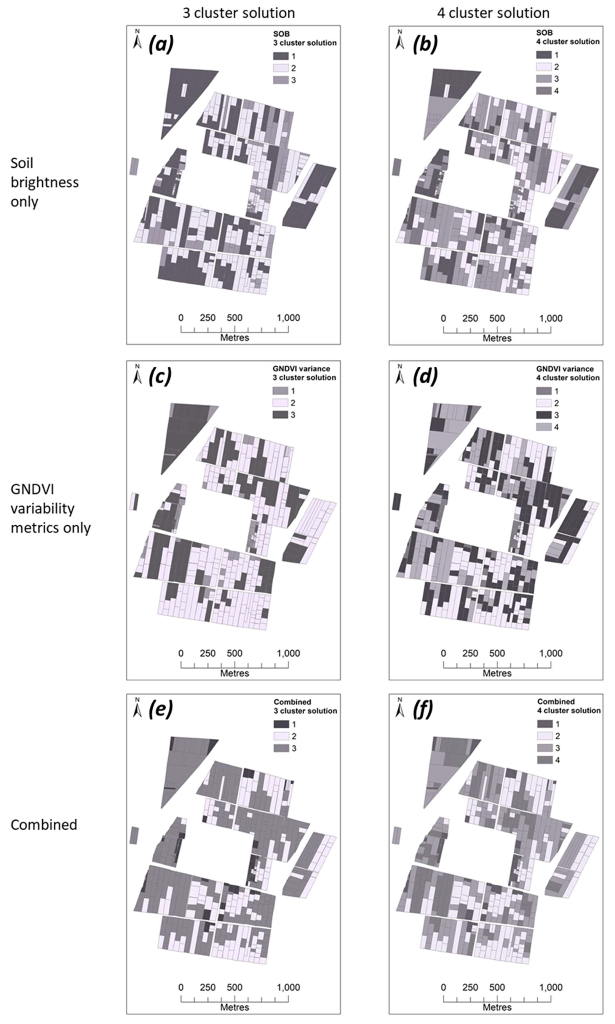
Figure 1. Location of the Wangzhaung village in China (red mark), the area occupied by the village (white polygon), and an image of the typical field layout in Wangzhuang village, China. The fields were separated only by a thin bare patch of soil. The similar growth stages of the wheat plants suggest that planting occurred at the same time in the different fields.
Agronomy 10 01767 g001
Figure 2. Maximum (full black line) and minimum (dotted black line) air temperature recorded at the Wangzhaung village from 2008 to 2018 from January to mid-May. The horizontal dotted line represents the 0 °C threshold while the vertical grey box represents the time when satellite images were acquired.
Agronomy 10 01767 g002
Figure 3. Calculated Green Normalized Vegetation Index (GNDVI) for LANDSAT 5 scenes for the growing season (a) 2008; (b) 2009; and (c) 2011. LANDSAT 5 scenes were obtained for late April/early May every year from 2008 to 2011.
Agronomy 10 01767 g003
Figure 4. Calculated GNDVI for LANDSAT 8 scenes for growing season (a) 2013; (b) 2015; and (c) 2018. LANDSAT 8 scenes were obtained for late April/early May from 2013 to 2018. There were no scenes available from 2012.
Agronomy 10 01767 g004
Figure 5. Soil brightness image (a) for 2017 resampled to match the LandSat8 spatial resolution (30 m) and (b) the original soil brightness image (3 m resolution).
Agronomy 10 01767 g005
Figure 6. Measured values of (a) soil nitrogen content (g/kg) and (b) soil organic carbon (%) at the field scale.
Agronomy 10 01767 g006
Figure 7. Ten-year time-series of GNDVI decomposed into (a) spatial variance and (b) temporal variance.
Agronomy 10 01767 g007
Figure 8. Results of clustering at field scale using (a,b) soil brightness alone; (c,d) the GNDVI variability metrics and (e,f) both combined, testing three and four cluster solutions.
Agronomy 10 01767 g008
Table 1. Relative variance of measured soil variables total N and organic carbon at the field scale for three and four cluster solutions using (i) soil brightness; (ii) the spatial and temporal variability in GNDVI and (iii) a combination of both.
Clustering ApproachRelative Variance (RV)
Total NOrganic Carbon
Soil brightness 3 zones7.57.3
Soil brightness 4 zones9.39.5
GNDVI variability metrics 3 zones35.837.3
GNDVI variability metrics 4 zones35.838.1
Combined 3 zones43.944.9
Combined 4 zones36.137.9
Publisher’s Note: MDPI stays neutral with regard to jurisdictional claims in published maps and institutional affiliations.

