Article

Assimilation of Sentinel-2 Estimated LAI into a Crop Model: Influence of Timing and Frequency of Acquisitions on Simulation of Water Stress and Biomass Production of Winter Wheat

1
Agrosphere (IBG-3), Institute of Bio- and Geosciences, Forschungszentrum Jülich, 52425 Jülich, Germany
2
Crop Science Research Group, Institute of Crop Science and Resource Conservation, University of Bonn, Katzenburgweg 5, 53115 Bonn, Germany
3
xarvioTM BASF Digital Farming GmbH, Im Zollhafen 24, 50678 Köln, Germany
*
Author to whom correspondence should be addressed.
Agronomy 2020, 10(11), 1813; https://doi.org/10.3390/agronomy10111813
Submission received: 13 August 2020 / Revised: 11 November 2020 / Accepted: 15 November 2020 / Published: 18 November 2020

Abstract

:
The Sentinel-2 (S2) Toolbox permits for the automated retrieval of leaf area index (LAI). LAI assimilation into crop simulation models could aid to improve the prediction accuracy for biomass at field level. We investigated if the combined effects of assimilation date and corresponding growth stage plus observational frequency have an impact on the crop model-based simulation of water stress and biomass production. We simulated winter wheat growth in nine fields in Germany over two years. S2 LAI estimations for each field were categorized into three phases, depending on the development stage of the crop at acquisition date (tillering, stem elongation, booting to flowering). LAI was assimilated in every possible combinational setup using the ensemble Kalman filter (EnKF). We evaluated the performance of the simulations based on the comparison of measured and simulated aboveground biomass at harvest. The results showed that the effects on water stress remained largely limited, because it mostly occurred after we stopped LAI assimilation. With regard to aboveground biomass, we found that the assimilation of only one LAI estimate from either the tillering or the booting to flowering stage resulted in simulated biomass values similar or closer to measured values than in those where more than one LAI estimate from the stem elongation phase were assimilated. LAI assimilation after the tillering phase might therefore be not necessarily required, as it may not lead to the desired improvement effect.

1. Introduction

Although originally developed for point-based applications that neglect spatial variation of weather, soil and management, dynamic crop simulation models have been increasingly used for field, regional, national and global scale purposes to simulate growth status, yield and soil–plant–atmosphere interactions of a variety of crops [1,2,3,4,5]. For precision agriculture applications, these models could help to guide the farmer in decisions related to site-specific management of crop input in terms of timing and amount [6] as well as the provision of spatially explicit yield forecasts [7]. In general, the reliability of crop growth simulations depends on the accurate representation of plant physiology processes in the model, the right selection of model parameters and the accuracy of the input data [8]. The performance is hampered by the uncertainty of those factors [9].
Modern remote sensing platforms and instruments enable one to capture biophysical crop canopy variables at spatial scales that allow for the recognition of variability within a field [10,11]. The assimilation of information on crop status and within-field variability into crop simulation models could help to limit the impact of poor model parameterization [9].
The idea of data assimilation in the context of dynamic crop models is to incorporate one or several observations of model state variables during the period of crop growth. Based on these measurements, the model can be updated or calibrated as to improve predictions about future states of the crop [12]. A number of different remote sensing-derived biophysical variables have been assimilated into crop models in the past, such as biomass [13], canopy cover [13,14], phenology [15,16], soil moisture [17,18,19,20,21] and, most-prominently used, leaf area index [14,15,18,19,20,22,23,24,25,26,27,28,29,30,31].
Multispectral optical satellite imagery is prevailingly used for the estimation of biophysical variables of vegetation (see [32] for a review). Technical constraints such as frequency of overpasses and cloud coverage, however, result in incomplete time series [33]. The amount and timing of biophysical variable estimations available for assimilation into crop models might therefore be different from location-to-location and year-to-year, as well as have an impact on the accuracy of the model predictions. Few studies investigated the impact of timing of state variable assimilation (i.e., leaf area index (LAI) and other variables) into crop models when simulating the growth of winter wheat. Huang et al. [25] found, relying on field-measured LAI, that (1) assimilating LAI during pre-heading stages achieved better model accuracy than assimilating LAI during post-heading stages, (2) when considering individual growth stages, LAI assimilation at heading played the most critical role, followed by booting, anthesis, elongation, jointing, green-up and maturity, and (3) the assimilation of LAI from all growth stages during the growing season resulted in the best accuracy. Xie et al. [20] found that the accuracy of yield estimation is highest when assimilating LAI at jointing and heading–filling stages as well as by assimilating soil moisture at green-up and milk stages, followed by the assimilation of LAI and soil moisture simultaneously and the assimilation of LAI alone. The authors assimilated one cloud-free Landsat image per main growth stage [20].
A number of studies have lately demonstrated the suitability of the Sentinel-2 (S2) multispectral imaging mission (operated by the European Space Agency (ESA)) to retrieve crop biophysical variables, including LAI, at high spatial resolution [34,35,36], and to plot within-field variability of crop status and growth as a foundation for precision farming applications [37,38,39,40].
Variable site characteristics typically cause within-field heterogeneity of crop growth and crop yields [41,42] because occurring stresses (e.g., water (=drought stress), heat, nutrient, diseases, ozone, etc.) hamper biomass development. In a recent study, we found that the inclusion of soil-related model variables in the data assimilation process is a promising approach for crop modeling at sub-field level under the consideration of simulated water stress [7]. We are currently not aware of any study that looks at the impacts of data assimilation into crop models that incorporate one or multiple stresses in their simulation routines, considering that typically only one or few state variables within a complex network of dependencies are updated during the procedure. Elaborate research is necessary to understand these consequences [7]. Based on these findings, we targeted the following research questions:
Does LAI (derived from Sentinel-2 imagery) assimilation into a crop model at different dates combined with their corresponding growth stages as well as the observational frequency have an impact on:
  • The simulation of water stress (as the ratio between the actual and the potential crop transpiration) in the crop model for nine conventionally farmed fields in Germany and,
  • The accuracy of winter wheat aboveground biomass predictions at harvest for those fields?

2. Materials and Methods
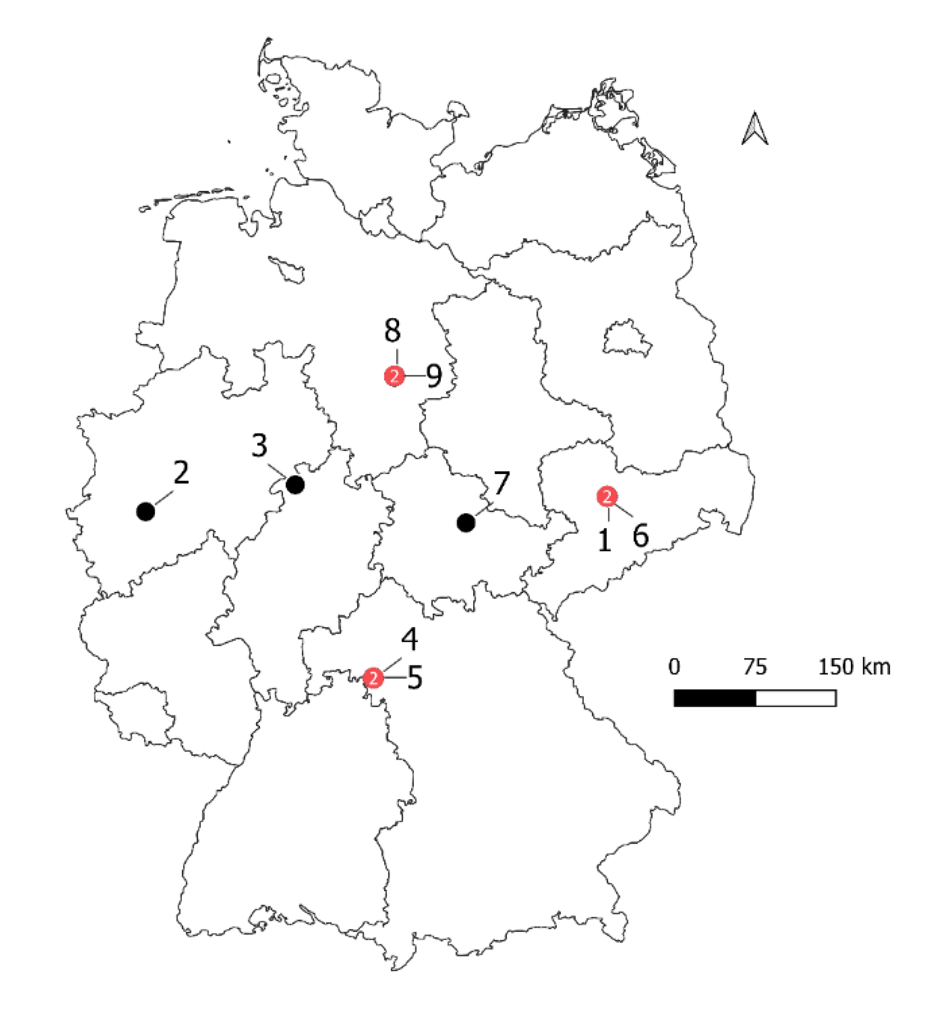
2.1. Field Data

Data from nine farmer fields sized between 7 hectares and 100 hectares across six states in Germany were included in this study. We grew winter wheat on three fields during the growing season 2016/2017, and on six fields during the growing season 2017/2018 (see Table 1 for an overview, and Figure A1 in the Appendix A for a map that indicates the locations). We selected commercial, widely available cultivars for seeding. Fertilizers, pesticides and growth regulators were applied based on best practice guidelines in accordance with local recommendations. The fields received no irrigation. Daily measurements of rainfall, minimum and maximum temperature at 2 m height, solar radiation and wind speed were logged by meteorological stations (Adcon Telemetry, Klosterneuburg, Austria) mounted in the immediate vicinity of the fields.
We distributed sampling points (between 20 and 48, depending on the size of the field) randomly across every field, where we sampled the soil in 30 cm intervals up to a depth of 90 cm. Texture composition (divided into the particle sizes sand, silt, clay and gravel according to the German soil classification [43]) and total organic carbon content were measured in the laboratory. Around maturity, we harvested aboveground biomass on a plot sized one square meter at each soil sampling point. Split into its components—grain, stem and leaves—each sample was oven-dried (at 105 °C) until we were unable to determine further weight reduction.
Average aboveground biomass yield per field varied between 12.13 t ha−1 (Field 7) and 19.34 t ha−1 (Field 3), the harvest index (i.e., the ratio of grain yield to total aboveground biomass as a measure of reproductive efficiency) varied between 0.41 (Field 2) and 0.58 (Field 1).

2.2. Crop Model Setup

We used the modeling framework SIMPLACE (Scientific Impact Assessment and Modelling Platform for Advanced Crop and Ecosystem Management—see Enders et al. [44] for general information on the framework, and www.simplace.net, accessed 29 May 2020) to simulate the growth of winter wheat in each sampling plot within each field. SIMPLACE modularizes crop model solutions into a number of software units (so-called SimComponents) that are discrete, replaceable and interchangeable [45]. Our study’s solution pooled the SimComponents LINTUL5, SlimRoots, SlimWater and STMPsim. LINTUL5 is a generic crop model that is able to simulate crop growth under potential, water limited and nitrogen, phosphorus and potassium limited growing conditions for many different annual crops [46]. It has been extensively employed to assess crop responses to various influences [3,47,48,49,50,51].
The total daily growth rate of the crop (=biomass development) in LINTUL5 is a function of daily temperature, intercepted radiation and radiation use efficiency (RUE). LAI is not simulated directly, but calculated daily as the product of specific leaf area (SLA, changes according to the development stage of the plant) and the weight of the living green leaves (WLVG—see the model’s documentation for more details [46]).
The SimComponent SlimWater was used to simulate the soil water balances for each sampling point. Based on the amount of crop water uptake, soil evaporation, surface run-off and seepage below the root zone, SlimWater simulates the daily change in soil water content in a one-dimensional, multiple layered soil profile [52]. The simulation of root growth was done using SlimRoots, where the daily increase in biomass of seminar and lateral roots depends on the input of assimilated biomass provided the shoot simulated in LINTUL5 (see Gaiser et al. [45] for more information). The SimComponent STMPsim calculated the soil temperature in each soil layer depending on weather and soil conditions.
We used the pedotransfer functions (PTFs) extracted from the database of hydraulic properties of European soils (HYPRES) [53] to predict soil hydraulic properties of each soil profile by fitting the Mualem-van-Genuchten model parameters, based on measured soil texture. HYPRES PTFs were developed based on soil hydraulic measurements provided by several organizations from 12 European countries. The applicability ranges over all of Europe [53]. We extended our soil profiles artificially down to 200 cm soil depth by copying the texture information that we had previously measured in the 60–90 cm soil depth layer.
As all fields were managed with the highest input level according to local recommendations (regarding pesticide and fertilizer application), no disease and nutrient stresses occurred. Water stress in our solution occurred if the simulated actual transpiration of the crop (TRAN in mm d−1) dropped below the simulated potential transpiration (PTRAN in mm d−1) due to insufficient levels of transpirable soil water in the root zone. Here, TRAN and PTRAN were calculated based on the modified Penman approach for the estimation of evapotranspiration [46]. In LINTUL5, water stress reduces the total daily growth rate of the crop by introducing a reduction factor computed as the ratio between TRAN and PTRAN [46]. Thus, at a given day when TRAN < PTRAN, the model simulation indicates occurrence of water stress, where the stress intensity depends on the ratio.
We ran SIMPLACE<LINTUL5,SLIM> in daily time steps. Data on daily phenology were requested from a xarvioTM in-house developed, commercial growth stage model (that replaced LINTUL’s internal phenology component), where the winter wheat cultivar-specific estimation was based on accumulated thermal temperature, vernalization and photoperiod. xarvioTM developed this model to provide better recommendations for fungicide application timing to farmers. It has been validated with roundabout 30,000 phenological observations from all over Germany.
Apart from phenology, we used the standard values for winter wheat, without consideration of cultivar specifics. In LINTUL5, phenology is determined by the development stage (DVS) of the plant, which ranges from 0 (seeding) over 1 (flowering) to 2 (fully ripe).

2.3. Sentinel-2 Leaf Area Index Estimations

We mapped LAI using the Sentinel Application Platform (SNAP) Sentinel-2 Toolbox Biophysical Processor for every field (see Table 1). Only those scenes were selected and atmospherically corrected using the Sen2Cor algorithm [54] where the conditions above the fields and the surrounding area were free of clouds. Here, LAI is defined as half the developed area of photosynthetically active elements (i.e., green, contributing elements such as stems and not just leaves) of the vegetation per unit horizontal ground area [55]. The Biophysical Processor tool permits for the automated per-pixel retrieval of essential climate variables (LAI, fraction of absorbed photosynthetically active radiation (FAPAR) and fraction of vegetation cover (FCOVER)) and other biophysical variables (chlorophyll content in the leaf and canopy water content) of any given vegetation type. These products are derived from the S2 top of canopy reflectance, without the inclusion of ancillary information from other sources (such as land cover information). Given this universal implementation, the processor’s estimations of LAI are therefore expected to be reasonably well across all vegetation types, but comparably worse than approaches developed for an explicit vegetation type [55].
Using bands 3–8a, 11 and 12 (bands with lower spatial resolution resampled to 10 m using the Nearest method implemented in SNAP) top of canopy reflectance data as input, the Biophysical Processor relies on a neural network (based on the generation of a training database using the PROSAIL radiative transfer model) to derive final LAI values [55]. For each assimilation step, we used the raster package [56] implemented in R [57] to extract LAI values from each pixel of the sampling points’ location.

2.4. Scenario Development

For this study, we categorized the S2 LAI images into three groups (phenophases, see Figure 1), depending on the DVS of the plants at the acquisition date of each S2 scene, as determined by the growth stage model for winter wheat (see Section 2.2). The first group (P1) encompassed the principal growth stage phase tillering (DVS < 0.44), the second group (P2) the phase stem elongation (0.44 ≥ DVS < 0.75), and the third group (P3) the phases booting, heading and flowering (0.75 ≥ DVS ≤ 1). For group 1, only one image was available per field and a maximum of four images each for groups 2 and 3.
Based on the maximum number of images available in each phenophase that could potentially be assimilated, we created every possible combinational setup for assimilation (Phenophase_1(0,1) × Phenophase_2(0,1,2,3,4) × Phenophase_3(0,1,2,3,4)) (Table 2) including the increments. We also included a model run where no LAI data were assimilated at all (combination 1, i.e., the control run without data assimilation, also referred to as open loop in other data assimilation publications), but relied solely on the calculation of the ensemble mean (EM, consisting of 100 members). We chose this option because previous studies showed that, among those options where no data were assimilated, the EM approach is able to outperform standard model runs [7,29].
Not every combination was possible for every field, due to a sometimes-lower maximum number of images available for P2 and/or P3. Images were randomly drawn within the different phenophases for those combinations where the number of images available for assimilation was smaller than the available number of images.
We did not include LAI estimations acquired after flowering (i.e., DVS > 1), since we intended to assess how suitable these approaches were for total aboveground biomass predictions at harvest (with simulation runs far beyond the assimilation of the last available estimation).

2.5. Model Run and LAI Assimilation

We ran SIMPLACE<LINTUL5,SLIM> in daily steps for all sampling points in all fields, using measured soil texture and weather data as model input. We used the ensemble Kalman filter (EnKF) to assimilate the S2-derived LAI information based on each combination into SIMPLACE <LINTUL5,SLIM>. LAI estimations in those combinations that contained more than one acquisition were assimilated in sequential order.
EnKF is a method that continuously updates the crop model whenever a new observation becomes available, based on the theory that improved simulation data at day t will increase the accuracy of the simulation data on subsequent days. It accounts for the uncertainty of the simulation results and observations, and pools an ensemble forecast and the Kalman filter to compute the prediction error covariance using a Monte Carlo method [58,59]. Evensen [60] provides in-depth information on EnKF.
Based on the findings of a previous study [7], the generation of the model ensemble (consisting of 100 members) relied on a set of three variables from soil and crop components of the model, which was deemed a good approach. A randomly generated Gaussian distribution was created for three variables: (1) the soil water content at simulation start (SoilWaterInit), (2) the maximal rooting depth of the plants (MaximalRootDepth) and (3) a scaling factor for SLA (ScaleFactorSLA). As we perturbed SoilWaterInit and MaximalRootDepth at the initialization of the simulation, water stress was induced by the model at differing points in time along the growing season. This resulted in the expansion of the range of LAI values in the ensemble at any given point in time. Neither SoilWaterInit nor MaximalRootDepth were updated during the simulations so as not to temper with the consistency of the model. SoilWaterInit was calculated for every soil layer k in the soil profile as:
S o i l W a t e r I n i t k = S c a l i n g F a c t o r V o l u m e t r i c W a t e r C o n t e n t 33 t o 1500 k + V o l u m e t r i c W a t e r C o n t e n t 1500 k
where VolumetricWaterContent33to1500 describes the volumetric soil water content from field capacity to wilting point (i.e., plant available water), and VolumetricWaterContent1500 the volumetric soil water content at permanent wilting point. Both values were returned by the PTF (Section 2.2), based on the measured soil texture. We included ScaleFactorSLA, scaling all predefined DVS-dependent SLA values uniformly in the set of ensemble generation variables, because it showed high impact on LAI dynamics and biomass accumulation in the model (as found in the sensitivity analysis, data not shown). No perturbation of other input data (e.g., weather data, reference evapotranspiration) was performed. Simulations were started the day that preceded the sowing day. We hereby achieved the maximum effect of varying soil water content in the model ensemble.
The LAI error was assumed to be 1. Whenever LAI was assimilated into SIMPLACE<LINTUL5,SLIM>, the state variable, WLVG, was adjusted by dividing LAI by SLA. This step ensured the consistency between LAI and dry matter of leaves as well as total aboveground biomass.
The entire workflow (i.e., simulation runs with different combinations of LAI assimilation) was repeated five times. This allowed us to investigate the influence of (a) the random distribution of values for the ensemble generation, and (b) the random drawing of images from the phenophases for those combinations where the number of images available for assimilation was smaller than the available number of images.

2.6. Evaluation of Model Performance

We based the evaluation of the model performance for each site and each combination tested on the comparison of measured and simulated total aboveground biomass at harvest day. Two metrics were calculated: the Root Mean Square Error (RMSE) and the Bias. RMSE indicated the magnitude of error in the unit of measurement. The Bias denoted the amount by which the predicted values were greater (positive Bias values) or smaller (negative Bias values) than the measured ones. Additionally, we calculated the difference between the cumulated mean actual crop transpiration (TRAN) and potential crop transpiration (PTRAN) (Section 2.2) per field for the period from planting to harvesting to study the effects of LAI assimilation on the initialization and intensity of water stress in the model simulations. The repetitions of this exercise (Section 2.5) allowed for the calculation of the standard deviation for every metric and combination.

3. Results

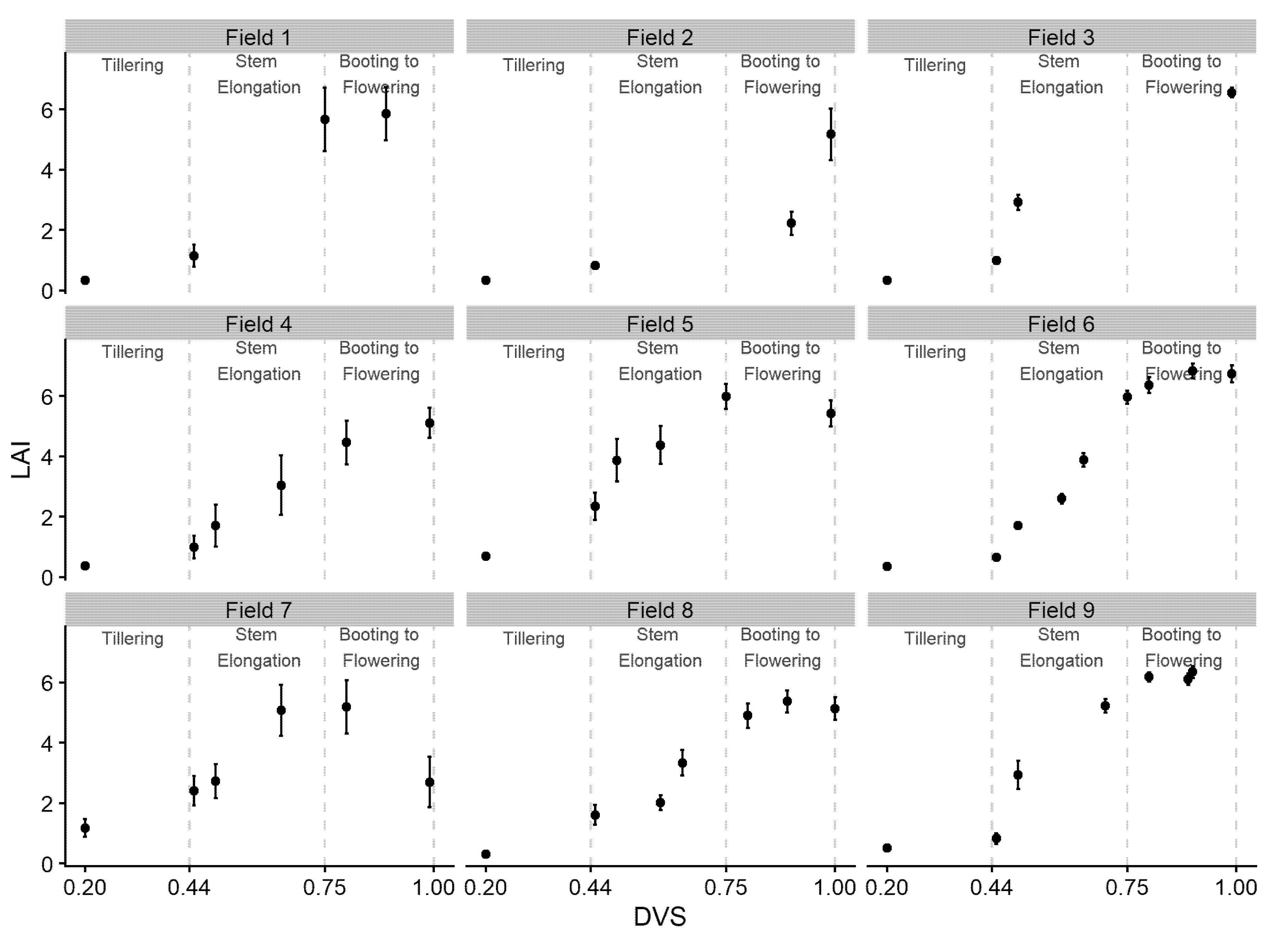
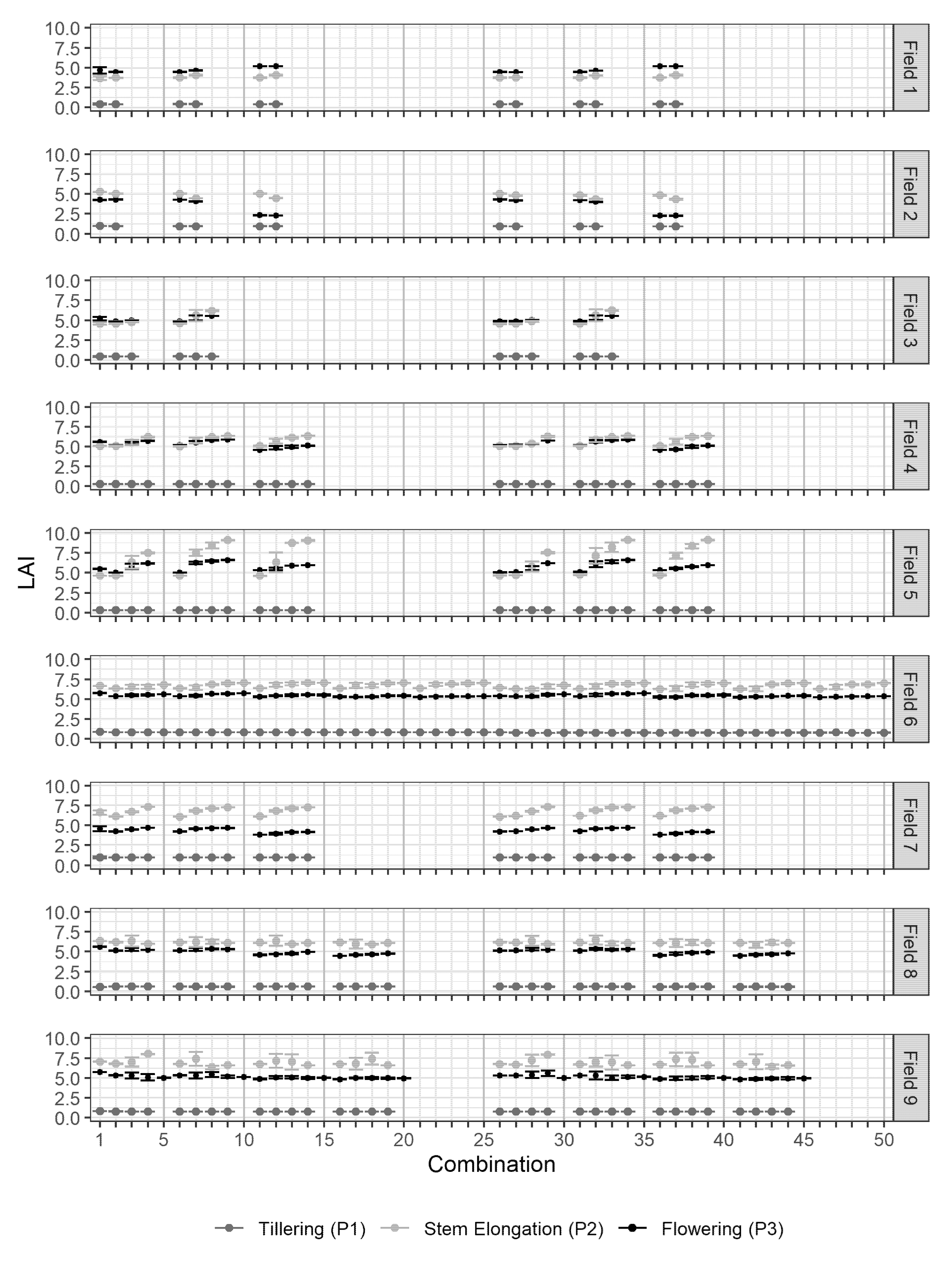
3.1. Sentinel-2 LAI Estimations and Simulated LAI

Figure 2 shows the average LAI development per field (plus standard deviation) until flowering stage, as extracted from the S2 imagery for all sampling points. Values ranged from LAI < 1 during the early phases of the growing season to maximum LAI > 5 during the later stages. Three fields show a clear reduction in LAI after peaking, even before the flowering stage (Fields 5, 8, and especially Field 7 with a very strong decrease in leaf area between acquisition dates 5 and 6), while the others showed sigmoid leaf growth (i.e., no reduction in LAI before flowering). In Field 2, a strong increase in leaf area index occurred only during the later phase of the booting to flowering stage.
The spatial heterogeneity of the S2-based LAI within the fields increased during the growing season, as indicated by the error bars that represent standard deviation (Figure 2). The levels of heterogeneity that developed differed between the fields, from low levels (Fields 3, 6 and 9, with a low spread during the growing season) to high levels (Fields 1, 4 and 7, high spread). In general, estimated LAI values were within reasonable, expectable ranges (see, e.g., Sieling et al. [61] to compare winter wheat LAI development).
Analysis of the average LAI states in the crop growth simulations for each field and combination (see Figure A2 in the Appendix A) at the end of the tillering phase (P1), end of stem elongation phase (P2) and end of flowering phase (P3) revealed the following: In comparison to the control run (combination 1, i.e., no LAI assimilation), LAI was only marginally in- or decreased by the updates until the end of the tillering stage. In most fields, LAI values at the end of the stem elongation phase (P2) exceeded those at the end of the booting to flowering stage (P3) in all combinations (see results for Fields 2, 6–9 in Figure A2 in the Appendix A). In other Fields (3–5), LAI values at the end of P2 and P3 were similar in some combinations (IDs 2–3, 6–8, 26–28) and diverged in others, where values at the end of P2 exceeded those at the end of P3 (IDs 12–14, 37–39). In Field 1, values at the end of the flowering stage (P3) exceeded those at the end of the stem elongation phase (P2) in all combinations. Especially the assimilation of estimates during P2 lead to substantial increases in LAI, which were only partly re-adjusted during P3.

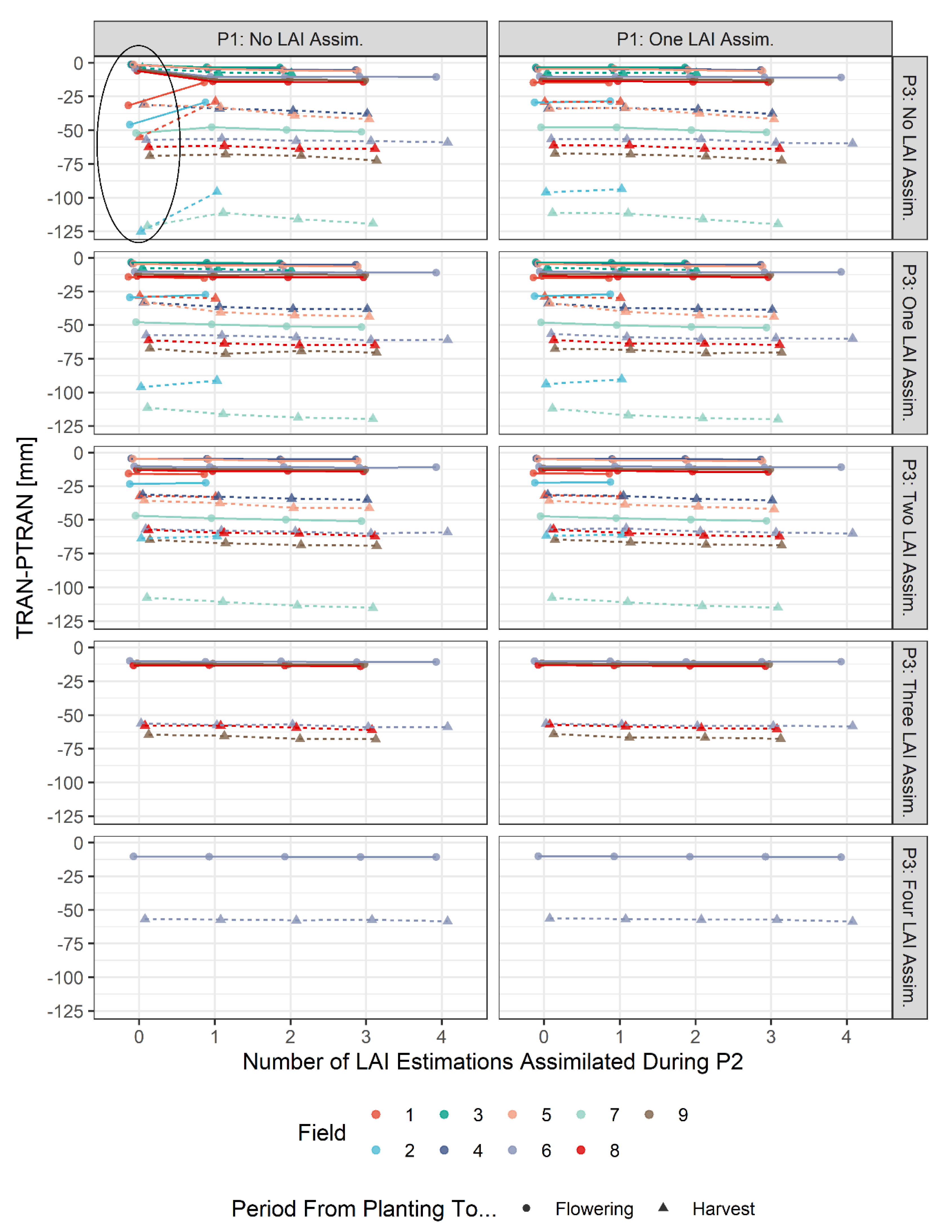
3.2. Results for Simulation of Water Stress

The assimilation of LAI estimations at different growth stages and with different frequencies affected the water stress levels in the simulations of our SIMPLACE<LINTUL5,SLIM> crop model solution to varying extents. In Figure 3, average water stress per field is indicated as the difference between mean actual crop transpiration TRAN and the mean potential crop transpiration PTRAN.
Until the flowering stage, LAI assimilation (during any phenophase) showed only minimal effects on water stress simulation in most fields (Fields 3–9). Values close to zero indicated that hardly any stress occurred in those simulations. In Fields 1 and 2, no LAI assimilation (see Figure 3, upper left panel) resulted in higher simulated water stress until flowering than in those simulations where LAI was assimilated.
During the period from planting to harvest, water stress in the model simulations was more pronounced (with up to 125 mm difference between TRAN and PTRAN), as suggested by the greater difference between TRAN and PTRAN (i.e., indicating a deficit of transpirable water). In most fields, the assimilation of LAI during P1 or P3 had an effect only if no LAI estimations from P2 were assimilated. The assimilation of LAI during P2 typically resulted in greater simulated stress than in those without simulations (except Fields 1 and 2), and an increasing number of estimations being assimilated resulted in even greater influence (Fields 3–9). In Fields 1 and 2, the assimilation during P2 decreased simulated stress, compared to the simulation without simulation.
The random selection of LAI retrievals for the assimilation had a limited impact on the TRAN and PTRAN results, as standard deviations were marginal among all fields and combinations. We therefore refrained from including the standard deviations in Figure 3.

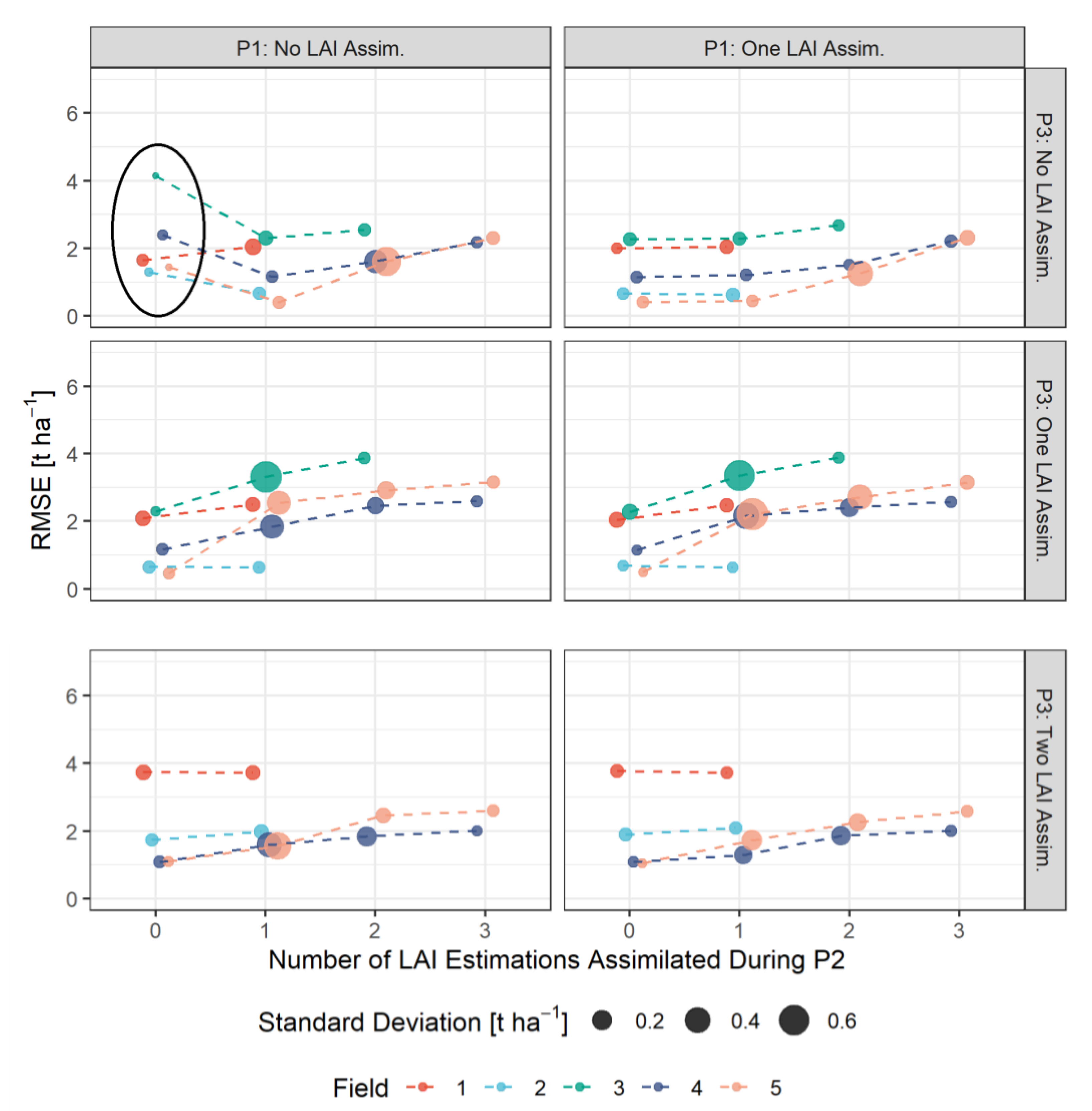
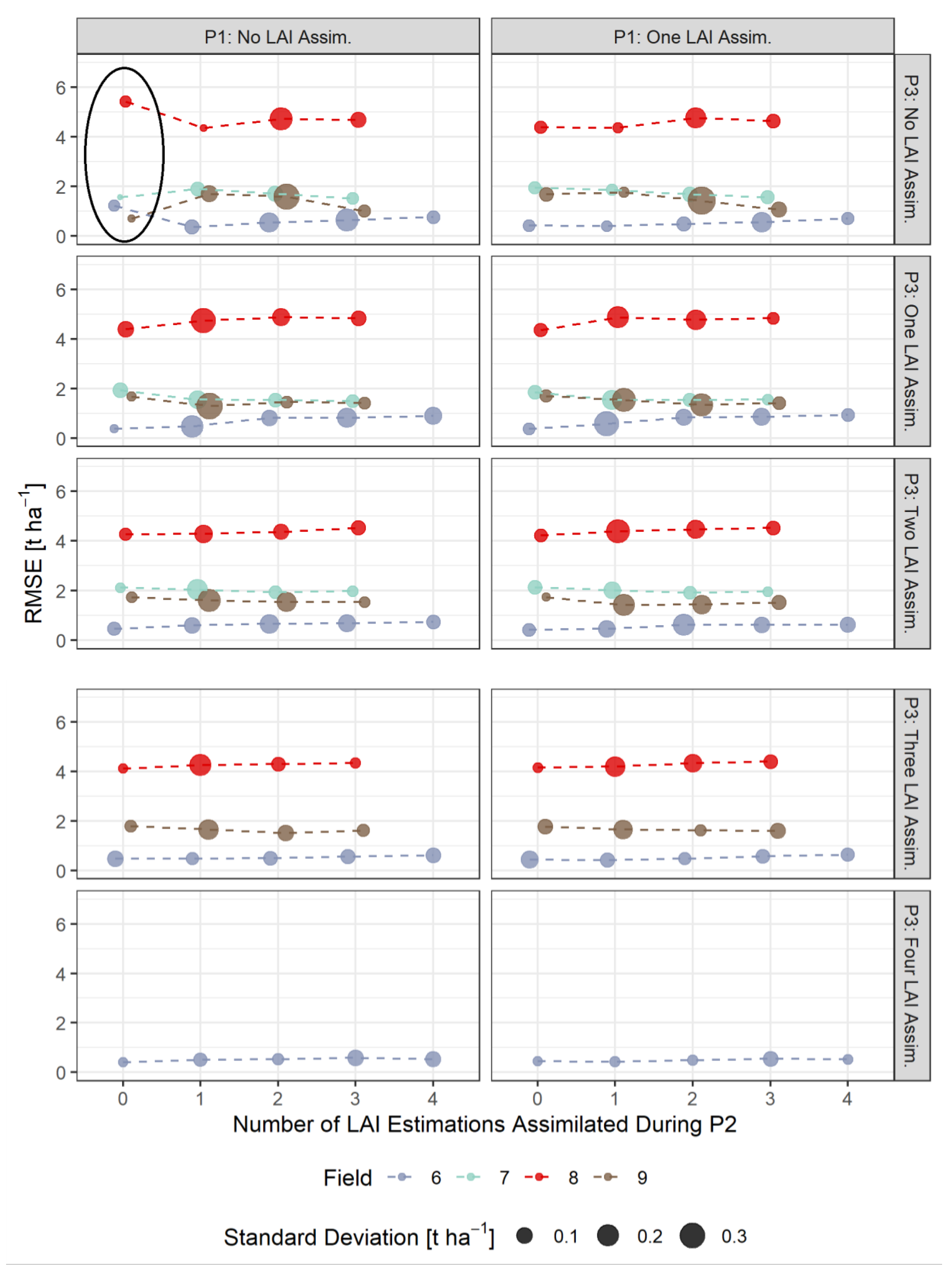
3.3. RMSE-Based Validation of Model Results

We calculated the RMSE of the total aboveground biomass per field, based on the comparison of simulated and measured total aboveground biomass at harvest day (Figure 4 for fields 1–5 and Figure 5 for fields 6–9). RMSE values ranged between 0.35 t ha−1 (Field 6, Combination 2) and 5.42 t ha−1 (Field 8, Combination 1). As are visible in Figure 4 and Figure 5, both the frequency of assimilations and the corresponding growth stage affected the performance of the model predictions. The assimilation of a single observation during P1 resulted in lower RMSE values compared to the control simulations (EM) in most fields (except Fields 1 and 9, where LAI assimilation always resulted in higher RMSE values). Similarly, the assimilation of one or more LAI estimations during P3 (and no LAI estimate from other periods) caused a reduction in RMSE in most of the fields, except in Fields 1 and 9. Looking at the influence of LAI assimilation during P2, we found that (1) RMSE decreased compared to the control run if no values from the earlier or later phenophases were assimilated and (2) the RMSE increased the more LAI estimates from P2 were assimilated. The randomization of LAI acquisition dates showed no significant effects on RMSE in Fields 1, 2, 6 and 7 (low standard deviation). Moderate to strong impacts were visible for some combinations in Fields 3, 4, 5 (Figure 4), 8 and 9 (Figure 5), particularly where LAI estimates from P2 were assimilated into the model runs.

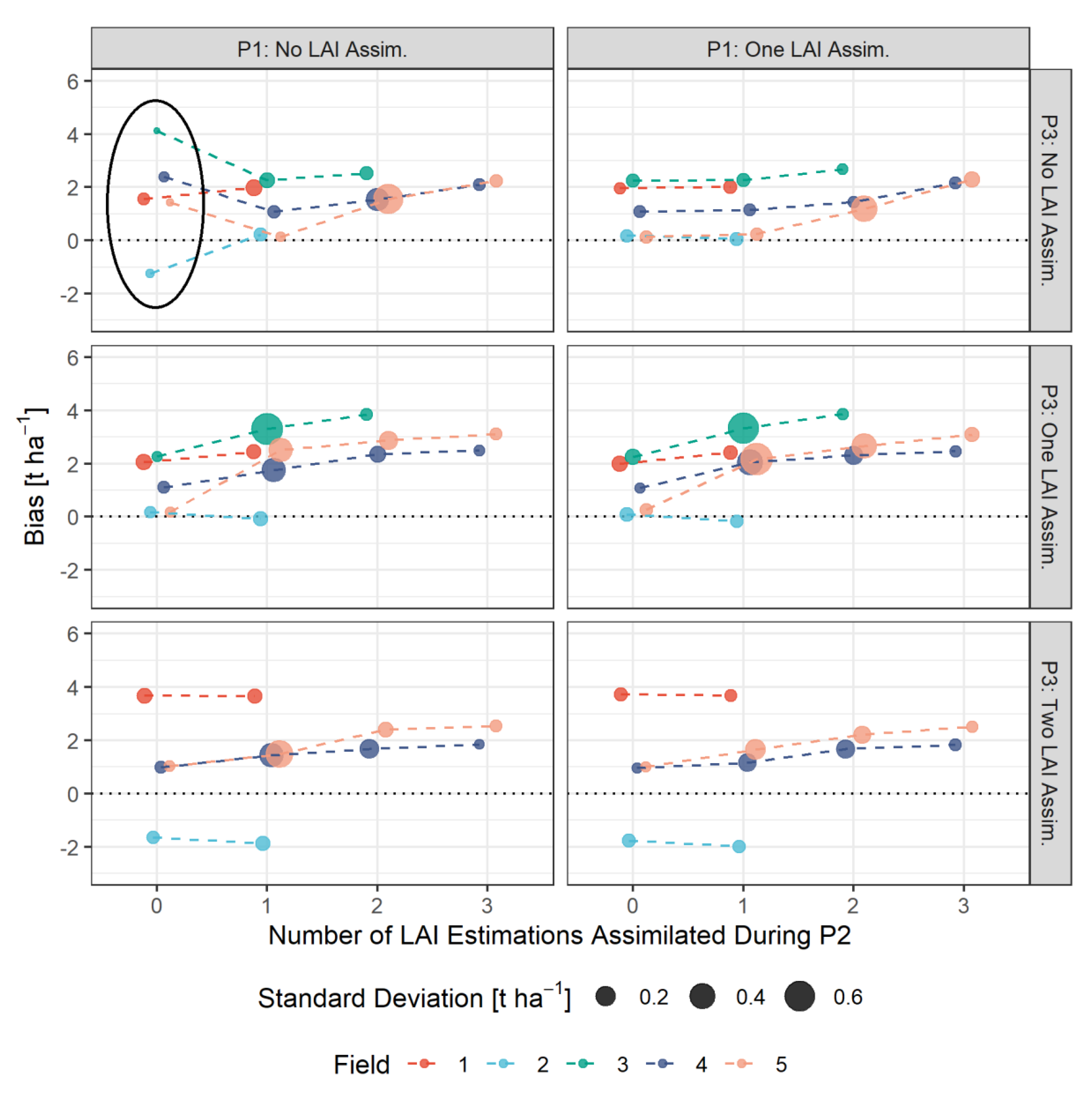
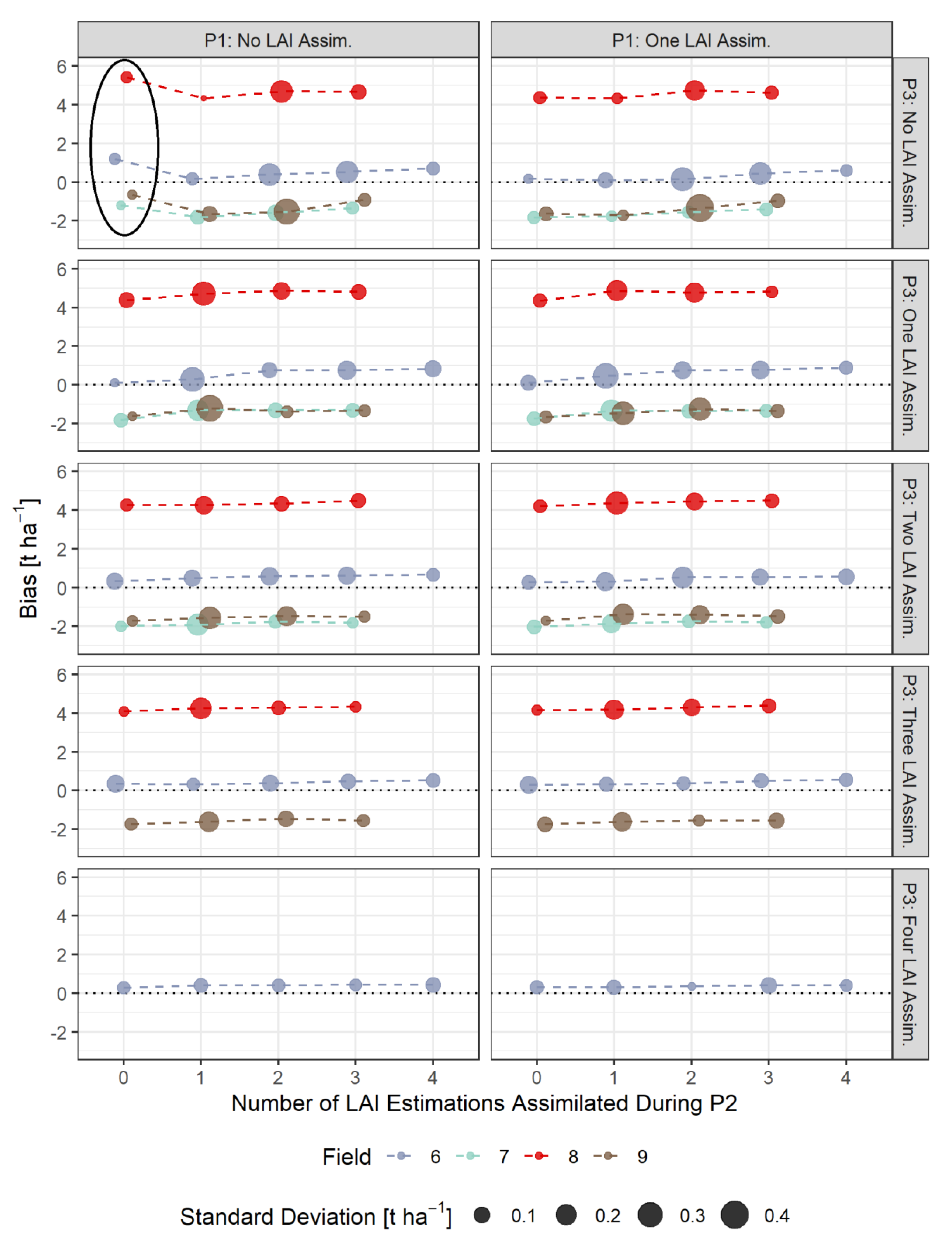
3.4. Bias-Based Validation of Model Results

The bias was calculated per field, based on the comparison of simulated and measured total aboveground biomass at harvest day (Figure 6 for fields 1–5 and Figure 7 for fields 6–9). A positive bias indicates overestimation of biomass by the crop model, a negative bias indicates underestimation. Mean bias ranged between −2.59 t ha−1 (Field 2, Combination 37) and 6.26 t ha−1 (Field 8, Combination 1). Values varied across combinations and across fields. In two fields (Fields 7 and 9), simulations underestimated measured total aboveground biomass in all combinations, and the bias of the control runs was closer to zero. In Field 2, different combinations caused either an over- or underestimation of measured biomass by the simulations. In all other fields (Fields 1, 3–6, 8), simulations overestimated measured biomass in all combinations. Similar to the RMSE results, the bias reduced, compared to the control run, when one LAI estimate from P1 or P3 was assimilated only (Fields 2–6, 8). The assimilation of LAI estimates from P2 caused the bias to increase; with a tendency to stronger deviate from 0 the more values were assimilated.
Contrary to this, Fields 7 and 9 showed a decrease in the bias when one or several images from P2 were used for the assimilation. The standard deviations tended to increase with an increasing number of LAI estimates from P2 that were assimilated into the simulation runs.

4. Discussion

4.1. Sentinel-2 LAI Estimations

We used the Biophysical Processor implemented in the SNAP Sentinel-2 Toolbox to derive LAI in the sampling plots in each field. Several studies reported on validation results of the Simplified Level 2 Product Prototype (i.e., a prior version of the Biophysical Processor that produces comparable results [55]) and reported satisfying results for the estimation of LAI (RMSE 0.80–0.98) for a variety of crops [62,63]. Recent publications examined the accuracy of the Biophysical Processor-estimated LAI in winter wheat [36,64] and durum wheat [64], and found varying results (winter wheat: RMSE 1.16–1.53, durum wheat: RMSE 0.74).
The authors of the algorithm emphasize that it is based upon a set of strong assumptions made by the PROSAIL radiative transfer model with regard to leaf optical properties, canopy structure and background reflectance. Results could be inaccurate if those assumptions are violated [55]. A custom correction that accounts for the specificities of the canopy type could be a solution to improve accuracy [55].
A number of publications have shown that automated S2-derived LAI estimations for winter wheat are within reasonable accuracies (see Section 2.3), with diverging tendencies. Pasqualotto et al. [63] found that the product tends to overestimate in-situ measured LAI, whereas Xie et al. [36] indicate a predisposition of the Biophysical Processor to underestimate LAI in the field. In his master thesis, Manuel Nolte (who co-authored this work) compared LAI measured in five winter wheat fields across Germany (different from ours) in 2019 using the LAI-2200C Plant Canopy Analyzer (LI-COR Inc., Lincoln, NE, USA) with Biophysical Processor-derived LAI based on Sentinel-2 imagery. He found that the software calculated higher LAI values than the measurement device (RMSE 1.13, R2 0.83), and that the Biophysical Processor outperformed a winter wheat-specific inversion of the PROSAIL model [65].
In our case, the LAI trajectories in Figure 2 look reasonable with respect to magnitude and dynamics in comparison to studies where LAI was measured in the field [25,61]. This underpins our confidence that Biophysical Processor-derived LAI adequately represents developments on the ground. Remaining uncertainty is encompassed during the assimilation process by our assumed LAI observation error of 1, justified by the findings in the above-mentioned publications.
Within our study, field-measured LAI data for the validation of the S2 estimations and the crop model results were not available. Given that high spatial resolution is a prerequisite for this study, we could not rely on other remote sensing-based automated LAI products (such as MODIS or SPOT), that typically offer information at coarser spatial resolution, for cross validation. Additionally, accurate and comprehensive LAI product validation exercises in the field are still very difficult due to the limitations of direct measurements [66].

4.2. Impacts of Combinations of LAI Assimilation on Simulation Results

The results for water stress (Section 3.2), RMSE (Section 3.3) and Bias (Section 3.4) clearly showed that the accuracy of the results was influenced by the timing and the frequency of LAI estimations that were assimilated into the SIMPLACE<LINTUL5,SLIM> crop model solution.
Figure 3 suggests that until the flowering stage, only minimal water stress occurred in the crop model simulations of most fields (except Fields 1 and 2), and that the magnitude of stress was not influenced by the assimilation of LAI estimates. Furthermore, the randomization of LAI estimations being assimilated within the same phenophases showed no effect on the simulation of neither potential nor actual transpiration, since the calculated standard deviation was negligible. Water stress therefore affected biomass production in those simulations only during the period between flowering and harvest (i.e., the period where the entire assimilate production is partitioned into the grain), where we did not assimilate any more LAI estimations. However, Figure 3 illustrates that the assimilation of LAI, especially during the stem elongation phase (P2) influenced the simulation of water stresses during the post-flowering period until harvest to a limited extent. However, we hypothesize that the effects of LAI assimilation might be more pronounced in those years where water stress occurs earlier during the growing season.
The results for Fields 1 and 2 constitute an exception to the rest of our findings, where the assimilation of at least one LAI estimate in P2 decreased the simulated stress dramatically, compared to the control run. While the reasons for Field 1 remain unclear, we assume that soil hydraulic properties were not represented adequately in Field 2, which caused an overestimation of water stress (resulting in an underestimation of biomass production, as visible in Figure 6).
The distinct decrease in S2-estimated LAI, even before flowering in Field 7 (Figure 2)—supported by the measured low amount of rainfall and a low harvest index (HI) (Table 1)—suggests the occurrence of strong water stress between the phases booting to flowering. The simulated water stress in Field 7 (see Figure 3) indicates a strong reduction in biomass production in the simulations that ultimately underestimated measured values in all cases. We therefore assume that our approach overestimated the stress that actually occurred in the field, despite the fact that LAI assimilation reduced stress levels (compared to the control run).
The results for the control runs (combination 1, encircled in Figure 3, Figure 4, Figure 5, Figure 6 and Figure 7) showed that our crop model solution overestimated true biomass production in most cases. Where updates (by the assimilation) caused major increases in LAI in the simulation runs (this occurred especially in those combinations where estimations from P2 were assimilated, see Figure A2 in the Appendix A), simulated water stress as well as biomass production increased. While this might seem contradictory at first, it adds up at second glance: A greater LAI increases the area of plant tissue that is photosynthetically active (i.e., causes the production of assimilates as well as the release of water from the leaves). This ultimately results in an increase in biomass production and water transpiration in the simulations. We assume that, in our case, the LAI assimilation caused a greater water stress in the simulations due to the increase in leaf area (as suggested in Figure 3). On the other hand, the increased biomass production caused by a greater LAI outweighed the reduction in production induced by increased water stress. The consequence of this causality was an overestimation of biomass production in most combinations of LAI assimilation, especially when more than one LAI estimate from P2 (stem elongation) were assimilated. However, combinations where solely LAI estimates from P1 and/or P3 were assimilated did not show this effect.
The major changes of simulated LAI caused by the assimilation of LAI estimates mostly occurred during the period of stem elongation (P2), where leaf area changes rapidly (see LAI dynamics during stem elongation phase in Figure 2). The greater standard deviations of RMSE and bias for those combinations where estimations from P2 were assimilated (compared to those where estimations from P3 were assimilated only) suggest that the timing of acquisition within P2 plays a stronger role for the prediction performance than for acquisitions within P3.
Except for Fields 1 and 9, the assimilation of only one LAI estimation from P1 produced RMSE and Bias values of aboveground biomass that were at least as good as those where more estimations from different points later in time during the growing season were assimilated (Figure 4, Figure 5, Figure 6 and Figure 7). This holds also true for the assimilation of one LAI estimation from P3. Our finding contrasts with the conclusions in other publications, where the assimilation of LAI from several growth stages produced better results, but lacked the consideration of plant stresses in the model runs [20,25].
While the majority of our results is in line with other studies, which found that the assimilation of S2-derived LAI into crop models improved the accuracy of the predictions in all cases [23,28], we also found that biomass estimations might actually deteriorate in spite of the assimilation of LAI, as the results for Fields 7 and 9 showed. While those two studies mentioned above focused on a spatially limited scale (experimental plots to farm level) with assumingly similar abiotic factors, we included data from fields that were distributed widely across Germany. In Fields 7 and 9, winter wheat was grown in 2017/2018 and the model performance in terms of RMSE as well as bias of the control run (i.e., no LAI assimilation) was best among all the nine fields. Thus, when taking the uncertainties of the LAI estimation procedure into account, no correction is needed, and it cannot be expected that the simulated total aboveground biomass will be improved by the assimilation procedure.
Another study [19] assimilated S2-derived LAI into the WOFOST crop model to simulate winter wheat biomass growth in 22 sampling plots across the Hebei Province, China. While the averaged results suggested that the assimilation improved prediction performance, a more detailed analysis of the results revealed that, similar to our findings, accuracy worsened with assimilation in some individual plots. Thus, the impact of the assimilation of LAI estimates on model outputs can be quite contrasting, when single fields over a larger region are compared. This fact may be due to spatially diverging quality of model input data (e.g., weather and soil data) or model-related weaknesses, which are site-specific.

4.3. Limitations of Input and Validation Data

Detailed, field-measured data were used as input into our solution (soil texture composition, meteorological data). Whilst we assume that these data represented actual conditions on-site as accurately as possible, it is not guaranteed that the most detailed input data improve model performance over input data that are less accurate [8,29]. Gridded worldwide weather, as well as soil texture data, is available, and we encourage researchers to investigate the impact of using these data in combination with remotely sensed LAI data.
We derived the soil hydraulic properties for each sampling point from pedotransfer functions published in the HYPRES database that is implemented in the SIMPLACE framework. Whilst some years have passed since the publication of HYPRES [53], we are aware of more recent developments in soil hydraulics modeling [67,68,69] that have not yet found their way into SIMPLACE. We therefore cannot make a statement whether the usage of other PTFs would yield more accurate modeling results when soil hydraulic properties were estimated by other pedotransfer functions. We encourage that future research should be devoted to the comparison of the impact of different PTFs.
With regard to model parameters, we considered differences in phenology as the only cultivar-specific properties. The model solution was not calibrated for other variables (e.g., SLA, RUE) that could have improved the results. Considering the scaling down of LAI values in the simulation runs between P2 and P3, even in fields where S2-estimated LAI showed no reduction (Figure 3), we assume that improper calibration/estimation of parameters that drove LAI development in our model solution caused an early LAI reduction in all ensemble members, which caused a reduction in the updated LAI by EnKF. It is therefore safe to say that the assimilation of LAI information into a crop model cannot compensate for all inadequacies.
We collected one aboveground biomass sample per sampling point in each field only for our validation exercise (i.e., we abstained from taking repetitive measurements). Although we worked diligently, measurements errors could have happened during the collection process. The readers should be aware of this uncertainty when interpreting the RMSE and Bias results.

5. Conclusions

In this study, we investigated if the assimilation of Sentinel-2-derived LAI estimations into the SIMPLACE<LINTUL5,SLIM> crop model using the ensemble Kalman filter (EnKF) in different phenophases and with varying timing and frequency had an impact on the simulation results of winter wheat growth in nine fields across Germany with regard to (a) the occurrence and magnitude of water stress and (b) the prediction accuracy of total aboveground biomass at harvest.
Given the range of factors that we incorporated in this study by running the crop model for different fields and years, the results allow one to draw conclusions for site-specific as well as general effects.
Both the timing and the frequency of LAI estimations influenced the simulation of water stress and biomass production to various extents. The effects on water stress simulation remained largely limited because they mostly occurred after flowering (where we stopped LAI assimilation). In comparison with the control run (i.e., no assimilation), LAI assimilation altered stress levels, but did not cause substantial changes with an increasing frequency of LAI assimilations. We found, however, that LAI assimilation (independent of the growing stage) changed stress levels substantially in two fields, which shows that the effect of LAI assimilation is site- and season-specific.
With regard to the biomass prediction performance, we found, to our surprise, that the assimilation of only one LAI estimate from either the tillering phase (P1) or the booting to flowering stage (P3) resulted in simulated biomass values that were similar or closer to measured values than in those simulations where more than one S2 LAI estimate was assimilated. The assimilation of estimates from the stem elongation phase (P2) largely caused a deterioration of the simulated biomass results. Here, the great magnitude of LAI value changes due to the assimilation of LAI estimates during the model runs caused a greater biomass production in the subsequent model steps, which, in turn, caused an increase in water stress that was outweighed by increased biomass production. Another important finding of this study was that LAI assimilation did not improve the model biomass predictions in all fields.
We would like to emphasize our key findings that are of interest to the crop modeling and data assimilation community as follows:
  • The assimilation of a single Sentinel-2-estimated LAI value derived during an early stage of crop development (tillering phase) had positive effects on the accuracy of the simulation of total crop biomass at harvest. Compared to those results, updating LAI with a greater frequency and at later growing stages did not result in improvements of the predictions. LAI assimilation after the tillering phase is therefore not necessarily required, as it may not lead to the desired effect.
  • The effects of LAI assimilation timing and frequency on water stress and biomass growth simulations might vary from site to site and season to season. We therefore encourage researchers to investigate and report those in detail, as to contribute to a better understanding of model responses.

Author Contributions

Conceptualization, A.T. and T.G.; methodology, A.T.; software, G.K.; validation, A.T., M.N. and H.H.; formal analysis, A.T.; investigation, A.T.; resources, H.H., M.N. and C.M.; data curation, H.H.; writing—original draft preparation, A.T.; writing—review and editing, C.M., M.N., G.K., H.H. and T.G.; visualization, A.T.; supervision, C.M., H.H. and T.G.; project administration, H.H.; funding acquisition, H.H. and C.M. All authors have read and agreed to the published version of the manuscript.

Funding

xarvioTM BASF Digital Farming GmbH, Köln, Germany funded this research. Andreas Tewes and Carsten Montzka additionally acknowledge support by Bundesministerium für Bildung und Forschung within the Agrarysteme der Zukunft—DAKIS project (Förderkennzeichen 031B0729F).

Acknowledgments

We thank Fabian Schäfer (xarvioTM) and Christian Kerkhoff (xarvioTM) for their valuable support.

Conflicts of Interest

The authors declare no conflict of interest.

Appendix A

Figure A1. Map of locations of study fields across Germany. Numbers correspond to field numbers in Table 1.
Agronomy 10 01813 g0a1
Figure A2. Average simulated LAI per field and combination at the end of the phases tillering (P1), stem elongation (P2) and flowering (P3). Error bars show standard deviation. See Table 2 for information about the composition of combinations.
Agronomy 10 01813 g0a2

References

  1. Eyshi Rezaei, E.; Siebert, S.; Ewert, F. Impact of data resolution on heat and drought stress simulated for winter wheat in Germany. Eur. J. Agron. 2015, 65, 69–82. [Google Scholar] [CrossRef]
  2. Maharjan, G.R.; Hoffmann, H.; Webber, H.; Srivastava, A.K.; Weihermüller, L.; Villa, A.; Coucheney, E.; Lewan, E.; Trombi, G.; Moriondo, M.; et al. Effects of input data aggregation on simulated crop yields in temperate and Mediterranean climates. Eur. J. Agron. 2019, 103, 32–46. [Google Scholar] [CrossRef]
  3. Mboh, C.M.; Srivastava, A.K.; Gaiser, T.; Ewert, F. Including root architecture in a crop model improves predictions of spring wheat grain yield and above-ground biomass under water limitations. J. Agron. Crop Sci. 2019, 205, 109–128. [Google Scholar] [CrossRef]
  4. Wallor, E.; Kersebaum, K.-C.; Ventrella, D.; Bindi, M.; Cammarano, D.; Coucheney, E.; Gaiser, T.; Garofalo, P.; Giglio, L.; Giola, P.; et al. The response of process-based agro-ecosystem models to within-field variability in site conditions. Field Crops Res. 2018, 228, 1–19. [Google Scholar] [CrossRef]
  5. Webber, H.; Gaiser, T.; Oomen, R.; Teixeira, E.; Zhao, G.; Wallach, D.; Zimmermann, A.; Ewert, F. Uncertainty in future irrigation water demand and risk of crop failure for maize in Europe. Environ. Res. Lett. 2016, 11, 074007. [Google Scholar] [CrossRef]
  6. Basso, B.; Ritchie, J.T.; Pierce, F.J.; Braga, R.P.; Jones, J.W. Spatial validation of crop models for precision agriculture. Agric. Syst. 2001, 68, 97–112. [Google Scholar] [CrossRef]
  7. Tewes, A.; Hoffmann, H.; Krauss, G.; Schäfer, F.; Kerkhoff, C.; Gaiser, T. New Approaches for the Assimilation of LAI Measurements into a Crop Model Ensemble to Improve Wheat Biomass Estimations. Agronomy 2020, 10, 446. [Google Scholar] [CrossRef] [Green Version]
  8. Waha, K.; Huth, N.; Carberry, P.; Wang, E. How model and input uncertainty impact maize yield simulations in West Africa. Environ. Res. Lett. 2015, 10, 024017. [Google Scholar] [CrossRef]
  9. Huang, J.; Gómez-Dans, J.L.; Huang, H.; Ma, H.; Wu, Q.; Lewis, P.E.; Liang, S.; Chen, Z.; Xue, J.-H.; Wu, Y.; et al. Assimilation of remote sensing into crop growth models: Current status and perspectives. Agric. For. Meteorol. 2019, 276–277, 107609. [Google Scholar] [CrossRef]
  10. Dong, T.; Shang, J.; Liu, J.; Qian, B.; Jing, Q.; Ma, B.; Huffman, T.; Geng, X.; Sow, A.; Shi, Y.; et al. Using RapidEye imagery to identify within-field variability of crop growth and yield in Ontario, Canada. Precis. Agric. 2019, 20, 1231–1250. [Google Scholar] [CrossRef]
  11. Kross, A.; McNairn, H.; Lapen, D.; Sunohara, M.; Champagne, C. Assessment of RapidEye vegetation indices for estimation of leaf area index and biomass in corn and soybean crops. Int. J. Appl. Earth Obs. Geoinf. 2015, 34, 235–248. [Google Scholar] [CrossRef] [Green Version]
  12. Wallach, D.; Makowski, D.; Jones, J.W.; Brun, F. Chapter 8-Data Assimilation for Dynamic Models. In Working with Dynamic Crop Models, 2nd ed.; Wallach, D., Makowski, D., Jones, J.W., Brun, F., Eds.; Academic Press: San Diego, CA, USA, 2014; pp. 311–343. ISBN 978-0-12-397008-4. [Google Scholar]
  13. Jin, X.; Li, Z.; Feng, H.; Ren, Z.; Li, S. Estimation of maize yield by assimilating biomass and canopy cover derived from hyperspectral data into the AquaCrop model. Agric. Water Manag. 2020, 227, 105846. [Google Scholar] [CrossRef]
  14. Silvestro, P.C.; Pignatti, S.; Pascucci, S.; Yang, H.; Li, Z.; Yang, G.; Huang, W.; Casa, R. Estimating Wheat Yield in China at the Field and District Scale from the Assimilation of Satellite Data into the Aquacrop and Simple Algorithm for Yield (SAFY) Models. Remote Sens. 2017, 9, 509. [Google Scholar] [CrossRef] [Green Version]
  15. Chen, Y.; Zhang, Z.; Tao, F. Improving regional winter wheat yield estimation through assimilation of phenology and leaf area index from remote sensing data. Eur. J. Agron. 2018, 101, 163–173. [Google Scholar] [CrossRef]
  16. Zhou, G.; Liu, X.; Liu, M. Assimilating Remote Sensing Phenological Information into the WOFOST Model for Rice Growth Simulation. Remote Sens. 2019, 11, 268. [Google Scholar] [CrossRef] [Green Version]
  17. De Wit, A.J.W.; van Diepen, C.A. Crop model data assimilation with the Ensemble Kalman filter for improving regional crop yield forecasts. Agric. For. Meteorol. 2007, 146, 38–56. [Google Scholar] [CrossRef]
  18. Ines, A.V.M.; Das, N.N.; Hansen, J.W.; Njoku, E.G. Assimilation of remotely sensed soil moisture and vegetation with a crop simulation model for maize yield prediction. Remote Sens. Environ. 2013, 138, 149–164. [Google Scholar] [CrossRef] [Green Version]
  19. Pan, H.; Chen, Z.; de Wit, A.; Ren, J. Joint Assimilation of Leaf Area Index and Soil Moisture from Sentinel-1 and Sentinel-2 Data into the WOFOST Model for Winter Wheat Yield Estimation. Sensors 2019, 19, 3161. [Google Scholar] [CrossRef] [Green Version]
  20. Xie, Y.; Wang, P.; Bai, X.; Khan, J.; Zhang, S.; Li, L.; Wang, L. Assimilation of the leaf area index and vegetation temperature condition index for winter wheat yield estimation using Landsat imagery and the CERES-Wheat model. Agric. For. Meteorol. 2017, 246, 194–206. [Google Scholar] [CrossRef]
  21. Zhuo, W.; Huang, J.; Li, L.; Zhang, X.; Ma, H.; Gao, X.; Huang, H.; Xu, B.; Xiao, X. Assimilating Soil Moisture Retrieved from Sentinel-1 and Sentinel-2 Data into WOFOST Model to Improve Winter Wheat Yield Estimation. Remote Sens. 2019, 11, 1618. [Google Scholar] [CrossRef] [Green Version]
  22. Dong, T.; Liu, J.; Qian, B.; Zhao, T.; Jing, Q.; Geng, X.; Wang, J.; Huffman, T.; Shang, J. Estimating winter wheat biomass by assimilating leaf area index derived from fusion of Landsat-8 and MODIS data. Int. J. Appl. Earth Obs. Geoinf. 2016, 49, 63–74. [Google Scholar] [CrossRef]
  23. Gilardelli, C.; Stella, T.; Confalonieri, R.; Ranghetti, L.; Campos-Taberner, M.; García-Haro, F.J.; Boschetti, M. Downscaling rice yield simulation at sub-field scale using remotely sensed LAI data. Eur. J. Agron. 2019, 103, 108–116. [Google Scholar] [CrossRef]
  24. Huang, J.; Ma, H.; Su, W.; Zhang, X.; Huang, Y.; Fan, J.; Wu, W. Jointly Assimilating Modis LAI and ET Products Into the SWAP Model for Winter Wheat Yield Estimation. IEEE J. Sel. Top. Appl. Earth Obs. Remote Sens. 2015, 8, 4060–4071. [Google Scholar] [CrossRef]
  25. Huang, J.; Tian, L.; Liang, S.; Ma, H.; Becker-Reshef, I.; Huang, Y.; Su, W.; Zhang, X.; Zhu, D.; Wu, W. Improving winter wheat yield estimation by assimilation of the leaf area index from Landsat TM and MODIS data into the WOFOST model. Agric. For. Meteorol. 2015, 204, 106–121. [Google Scholar] [CrossRef] [Green Version]
  26. Li, H.; Chen, Z.; Liu, G.; Jiang, Z.; Huang, C. Improving Winter Wheat Yield Estimation from the CERES-Wheat Model to Assimilate Leaf Area Index with Different Assimilation Methods and Spatio-Temporal Scales. Remote Sens. 2017, 9, 190. [Google Scholar] [CrossRef] [Green Version]
  27. Mokhtari, A.; Noory, H.; Vazifedoust, M. Improving crop yield estimation by assimilating LAI and inputting satellite-based surface incoming solar radiation into SWAP model. Agric. For. Meteorol. 2018, 250–251, 159–170. [Google Scholar] [CrossRef]
  28. Novelli, F.; Spiegel, H.; Sandén, T.; Vuolo, F. Assimilation of Sentinel-2 Leaf Area Index Data into a Physically-Based Crop Growth Model for Yield Estimation. Agronomy 2019, 9, 255. [Google Scholar] [CrossRef] [Green Version]
  29. Tewes, A.; Hoffmann, H.; Nolte, M.; Krauss, G.; Schäfer, F.; Kerkhoff, C.; Gaiser, T. How Do Methods Assimilating Sentinel-2-Derived LAI Combined with Two Different Sources of Soil Input Data Affect the Crop Model-Based Estimation of Wheat Biomass at Sub-Field Level? Remote Sens. 2020, 12, 925. [Google Scholar] [CrossRef] [Green Version]
  30. Xie, Y.; Wang, P.; Sun, H.; Zhang, S.; Li, L. Assimilation of Leaf Area Index and Surface Soil Moisture With the CERES-Wheat Model for Winter Wheat Yield Estimation Using a Particle Filter Algorithm. IEEE J. Sel. Top. Appl. Earth Obs. Remote Sens. 2017, 10, 1303–1316. [Google Scholar] [CrossRef]
  31. Zhao, Y.; Chen, S.; Shen, S. Assimilating remote sensing information with crop model using Ensemble Kalman Filter for improving LAI monitoring and yield estimation. Ecol. Model. 2013, 270, 30–42. [Google Scholar] [CrossRef]
  32. Fang, H.; Baret, F.; Plummer, S.; Schaepman-Strub, G. An Overview of Global Leaf Area Index (LAI): Methods, Products, Validation, and Applications. Rev. Geophys. 2019, 57, 739–799. [Google Scholar] [CrossRef]
  33. Weiss, M.; Jacob, F.; Duveiller, G. Remote sensing for agricultural applications: A meta-review. Remote Sens. Environ. 2020, 236, 111402. [Google Scholar] [CrossRef]
  34. Clevers, J.G.P.W.; Kooistra, L.; Van den Brande, M.M.M. Using Sentinel-2 Data for Retrieving LAI and Leaf and Canopy Chlorophyll Content of a Potato Crop. Remote Sens. 2017, 9, 405. [Google Scholar] [CrossRef] [Green Version]
  35. Pasqualotto, N.; Delegido, J.; Van Wittenberghe, S.; Rinaldi, M.; Moreno, J. Multi-Crop Green LAI Estimation with a New Simple Sentinel-2 LAI Index (SeLI). Sensors 2019, 19, 904. [Google Scholar] [CrossRef] [Green Version]
  36. Xie, Q.; Dash, J.; Huete, A.; Jiang, A.; Yin, G.; Ding, Y.; Peng, D.; Hall, C.C.; Brown, L.; Shi, Y.; et al. Retrieval of crop biophysical parameters from Sentinel-2 remote sensing imagery. Int. J. Appl. Earth Obs. Geoinformation 2019, 80, 187–195. [Google Scholar] [CrossRef]
  37. Fieuzal, R.; Bustillo, V.; Collado, D.; Dedieu, G. Combined Use of Multi-Temporal Landsat-8 and Sentinel-2 Images for Wheat Yield Estimates at the Intra-Plot Spatial Scale. Agronomy 2020, 10, 327. [Google Scholar] [CrossRef] [Green Version]
  38. Pause, M.; Raasch, F.; Marrs, C.; Csaplovics, E. Monitoring Glyphosate-Based Herbicide Treatment Using Sentinel-2 Time Series—A Proof-of-Principle. Remote Sens. 2019, 11, 2541. [Google Scholar] [CrossRef] [Green Version]
  39. Toscano, P.; Castrignanò, A.; Di Gennaro, S.F.; Vonella, A.V.; Ventrella, D.; Matese, A. A Precision Agriculture Approach for Durum Wheat Yield Assessment Using Remote Sensing Data and Yield Mapping. Agronomy 2019, 9, 437. [Google Scholar] [CrossRef] [Green Version]
  40. Vizzari, M.; Santaga, F.; Benincasa, P. Sentinel 2-Based Nitrogen VRT Fertilization in Wheat: Comparison between Traditional and Simple Precision Practices. Agronomy 2019, 9, 278. [Google Scholar] [CrossRef] [Green Version]
  41. Brogi, C.; Huisman, J.A.; Herbst, M.; Weihermüller, L.; Klosterhalfen, A.; Montzka, C.; Reichenau, T.G.; Vereecken, H. Simulation of spatial variability in crop leaf area index and yield using agroecosystem modeling and geophysics-based quantitative soil information. Vadose Zone J. 2020, 19. [Google Scholar] [CrossRef] [Green Version]
  42. Pätzold, S.; Mertens, F.M.; Bornemann, L.; Koleczek, B.; Franke, J.; Feilhauer, H.; Welp, G. Soil heterogeneity at the field scale: A challenge for precision crop protection. Precis. Agric. 2008, 9, 367–390. [Google Scholar] [CrossRef]
  43. Eckelmann, W.; Sponagel, H.; Grottenthaler, W.; Hartmann, K.-J.; Hartwich, R.; Janetzko, P.; Joisten, H.; Kühn, D.; Sabel, K.-J.; Traidl, R. Bodenkundliche Kartieranleitung. KA5; Bundesanstalt für Geowissenschaften und Rohstoffe, Ed.; Schweizerbart Science Publishers: Stuttgart, Germany, 2006; ISBN 978-3-510-95920-4. [Google Scholar]
  44. Enders, A.; Diekkrüger, B.; Laudien, R.; Gaiser, T.; Bareth, G. The IMPETUS Spatial Decision Support Systems. In Impacts of Global Change on the Hydrological Cycle in West and Northwest Africa; Speth, P., Christoph, M., Diekkrüger, B., Eds.; Springer: Berlin/Heidelberg, Germany, 2010; pp. 360–393. ISBN 978-3-642-12957-5. [Google Scholar]
  45. Gaiser, T.; Perkons, U.; Küpper, P.M.; Kautz, T.; Uteau-Puschmann, D.; Ewert, F.; Enders, A.; Krauss, G. Modeling biopore effects on root growth and biomass production on soils with pronounced sub-soil clay accumulation. Ecol. Model. 2013, 256, 6–15. [Google Scholar] [CrossRef]
  46. Wolf, J. User Guide for LINTUL5: Simple Generic Model for Simulation of Crop Growth under Potential, Water Limited and Nitrogen, Phosphorus and Potassium Limited Conditions; Wageningen UR: Wageningen, The Netherlands, 2012. [Google Scholar]
  47. Faye, B.; Webber, H.; Diop, M.; Mbaye, M.L.; Owusu-Sekyere, J.D.; Naab, J.B.; Gaiser, T. Potential impact of climate change on peanut yield in Senegal, West Africa. Field Crop. Res. 2018, 219, 148–159. [Google Scholar] [CrossRef]
  48. Gabaldón-Leal, C.; Webber, H.; Otegui, M.E.; Slafer, G.A.; Ordóñez, R.A.; Gaiser, T.; Lorite, I.J.; Ruiz-Ramos, M.; Ewert, F. Modelling the impact of heat stress on maize yield formation. Field Crop. Res. 2016, 198, 226–237. [Google Scholar] [CrossRef]
  49. Srivastava, A.K.; Ceglar, A.; Zeng, W.; Gaiser, T.; Mboh, C.M.; Ewert, F. The Implication of Different Sets of Climate Variables on Regional Maize Yield Simulations. Atmosphere 2020, 11, 180. [Google Scholar] [CrossRef] [Green Version]
  50. Srivastava, A.K.; Mboh, C.M.; Gaiser, T.; Kuhn, A.; Ermias, E.; Ewert, F. Effect of mineral fertilizer on rain water and radiation use efficiencies for maize yield and stover biomass productivity in Ethiopia. Agric. Syst. 2019, 168, 88–100. [Google Scholar] [CrossRef]
  51. Webber, H.; Zhao, G.; Wolf, J.; Britz, W.; de Vries, W.; Gaiser, T.; Hoffmann, H.; Ewert, F. Climate change impacts on European crop yields: Do we need to consider nitrogen limitation? Eur. J. Agron. 2015, 71, 123–134. [Google Scholar] [CrossRef]
  52. Addiscott, T.M.; Whitmore, A.P. Simulation of solute leaching in soils of differing permeabilities. Soil Use Manag. 1991, 7, 94–102. [Google Scholar] [CrossRef]
  53. Wösten, J.H.M.; Lilly, A.; Nemes, A.; Le Bas, C. Development and use of a database of hydraulic properties of European soils. Geoderma 1999, 90, 169–185. [Google Scholar] [CrossRef]
  54. Main-Knorn, M.; Pflug, B.; Louis, J.; Debaecker, V.; Müller-Wilm, U.; Gascon, F. Sen2Cor for Sentinel-2. In Proceedings of the Image and Signal Processing for Remote Sensing XXIII, Warsaw, Poland, 11–13 September 2017; Bruzzone, L., Bovolo, F., Benediktsson, J.A., Eds.; SPIE: Warsaw, Poland, 2017; p. 3. [Google Scholar]
  55. Weiss, M.; Baret, F. S2ToolBox Level 2 Products: LAI, FAPAR, FCOVER. Sentinel-2 Algorithm Theoretical Based Document. Available online: http://step.esa.int/docs/extra/ATBD_S2ToolBox_L2B_V1.1.pdf (accessed on 13 August 2020).
  56. Hijmans, R.J. Raster: Geographic Data Analysis and Modeling; Scientific Research Publishing (SCIRP): Irvine, CA, USA, 2020. [Google Scholar]
  57. R Core Team. R: A Language and Environment for Statistical Computing; R Foundation for Statistical Computing: Vienna, Austria, 2019. [Google Scholar]
  58. Guo, C.; Tang, Y.; Lu, J.; Zhu, Y.; Cao, W.; Cheng, T.; Zhang, L.; Tian, Y. Predicting wheat productivity: Integrating time series of vegetation indices into crop modeling via sequential assimilation. Agric. For. Meteorol. 2019, 272–273, 69–80. [Google Scholar] [CrossRef]
  59. Jin, X.; Kumar, L.; Li, Z.; Feng, H.; Xu, X.; Yang, G.; Wang, J. A review of data assimilation of remote sensing and crop models. Eur. J. Agron. 2018, 92, 141–152. [Google Scholar] [CrossRef]
  60. Evensen, G. The Ensemble Kalman Filter: Theoretical formulation and practical implementation. Ocean Dyn. 2003, 53, 343–367. [Google Scholar] [CrossRef]
  61. Sieling, K.; Böttcher, U.; Kage, H. Dry matter partitioning and canopy traits in wheat and barley under varying N supply. Eur. J. Agron. 2016, 74, 1–8. [Google Scholar] [CrossRef]
  62. Djamai, N.; Fernandes, R.; Weiss, M.; McNairn, H.; Goïta, K. Validation of the Sentinel Simplified Level 2 Product Prototype Processor (SL2P) for mapping cropland biophysical variables using Sentinel-2/MSI and Landsat-8/OLI data. Remote Sens. Environ. 2019, 225, 416–430. [Google Scholar] [CrossRef]
  63. Pasqualotto, N.; Bolognesi, S.F.; Belfiore, O.R.; Delegido, J.; D’Urso, G.; Moreno, J. Canopy chlorophyll content and LAI estimation from Sentine1-2: Vegetation indices and Sentine1-2 Leve1-2A automatic products comparison. In Proceedings of the 2019 IEEE International Workshop on Metrology for Agriculture and Forestry (MetroAgriFor), Portici, Italy, 24–26 October 2019; pp. 301–306. [Google Scholar]
  64. Upreti, D.; Huang, W.; Kong, W.; Pascucci, S.; Pignatti, S.; Zhou, X.; Ye, H.; Casa, R. A Comparison of Hybrid Machine Learning Algorithms for the Retrieval of Wheat Biophysical Variables from Sentinel-2. Remote Sens. 2019, 11, 481. [Google Scholar] [CrossRef] [Green Version]
  65. Nolte, M. Retrieval of Leaf Area Index for Field Crops with the Radiative Transfer Model PROSAIL. Master’s Thesis, University of Bonn, Bonn, Germany, 2019. [Google Scholar]
  66. Yan, G.; Hu, R.; Luo, J.; Weiss, M.; Jiang, H.; Mu, X.; Xie, D.; Zhang, W. Review of indirect optical measurements of leaf area index: Recent advances, challenges, and perspectives. Agric. For. Meteorol. 2019, 265, 390–411. [Google Scholar] [CrossRef]
  67. Montzka, C.; Herbst, M.; Weihermüller, L.; Verhoef, A.; Vereecken, H. A global data set of soil hydraulic properties and sub-grid variability of soil water retention and hydraulic conductivity curves. Earth Syst. Sci. Data 2017, 9, 529–543. [Google Scholar] [CrossRef] [Green Version]
  68. Tóth, B.; Weynants, M.; Pásztor, L.; Hengl, T. 3D soil hydraulic database of Europe at 250 m resolution. Hydrol. Process. 2017, 31, 2662–2666. [Google Scholar] [CrossRef] [Green Version]
  69. Tóth, B.; Weynants, M.; Nemes, A.; Makó, A.; Bilas, G.; Tóth, G. New generation of hydraulic pedotransfer functions for Europe: New hydraulic pedotransfer functions for Europe. Eur. J. Soil Sci. 2015, 66, 226–238. [Google Scholar] [CrossRef]
Figure 1. Available cloud-free Sentinel-2 images per field for leaf area index (LAI) estimation, with the acquisition dates converted to development stages (DVS) of winter wheat. A cross indicates each available image (×). DVS 0.2: beginning of tillering; 0.5: beginning of stem elongation; 0.9: beginning of heading; 1: full flowering. Dashed vertical lines represent phenophase ranges.
Agronomy 10 01813 g001
Figure 2. Average LAI development (as development stage DVS) per field until flowering stage, as extracted from the Sentinel-2 imagery. Error bars show standard deviation. DVS 0.2: beginning of tillering; 0.5: beginning of stem elongation; 0.9: beginning of heading; 1: full flowering. Dashed vertical lines represent phenophase ranges.
Agronomy 10 01813 g002
Figure 3. Difference between mean actual crop transpiration (TRAN, in mm) and potential crop transpiration (PTRAN, in mm) for Fields 1–9 as calculated by the crop model, cumulated for the period from planting to flowering and planting to harvest. Matrix of panels defined by the number of LAI estimations assimilated during phenophase 1 (P1, columns) and the number of LAI estimations assimilated during phenophase 3 (P3, rows), with the number of LAI estimations assimilated during phenophase 2 (P2) indicated on the horizontal axis. Encircled points indicate results of the control run (i.e., no LAI assimilation). Repeated model runs showed a marginal effect on Root Mean Square Error (RMSE) only, which is why we do not provide the standard deviation. For improved readability, the horizontal positions of the points are slightly dodged.
Agronomy 10 01813 g003
Figure 4. Mean RMSE of total aboveground biomass predictions for fields 1–5. Matrix of panels defined by the number of LAI estimations assimilated during phenophase 1 (P1, columns) and the number of LAI estimations assimilated during phenophase 3 (P3, rows), with the number of LAI estimations assimilated during phenophase 2 (P2) indicated on the horizontal axis. Point sizes indicate standard deviation. Encircled points indicate results of the control run (i.e., no LAI assimilation). See Table 2 for information about combinations. RMSE in t ha−1. See Figure 5 for results of fields 6–9.
Agronomy 10 01813 g004
Figure 5. Mean RMSE of total aboveground biomass predictions for fields 6–9. See caption of Figure 4 for further explanations.
Agronomy 10 01813 g005
Figure 6. Mean Bias of total aboveground biomass prediction for fields 1–5. Matrix of panels defined by the number of LAI estimations assimilated during phenophase 1 (P1, columns) and the number of LAI estimations assimilated during phenophase 3 (P3, rows), with the number of LAI estimations assimilated during phenophase 2 (P2) indicated on the horizontal axis. Point sizes indicate standard deviation. Encircled points indicate results of the control run (i.e., no LAI assimilation). See Table 2 for information about combinations. Positive values indicate overestimation by the model. Bias in t ha−1. See Figure 7 for results of fields 6–9.
Agronomy 10 01813 g006
Figure 7. Mean Bias of total aboveground biomass predictions for fields 6–9. See caption of Figure 6 for further explanations.
Agronomy 10 01813 g007
Table 1. List of fields and their respective locations in Germany. BMY: average total aboveground biomass yield (t ha−1), GY: average grain yield (t ha−1), HI: harvest index (=GY/BMY), SN: Saxony, NW: North Rhine-Westphalia, HE: Hesse, BY: Bavaria, TH: Thuringia, NI: Lower Saxony. Sum of rainfall (mm) between planting and harvest.
Growing SeasonFieldLocation Within StateName of CultivarPlanting DateBMYGYHINo of Sampling PointsSum Rainfall
2016/20171SNBenchmark30 November 201616.319.430.5830329
2016/20172NWJonny25 October 201614.515.960.4129393
2016/20173HEJulius28 October 201619.349.850.5120496
2017/20184BYRGT Reform3 November 201714.517.740.5348353
2017/20185BYRGT Reform16 November 201716.418.090.4944324
2017/20186SNRGT Reform16 October 201718.829.540.5121352
2017/20187THRGT Reform19 October 201712.135.180.4338214
2017/20188NIRGT Reform3 November 201714.528.080.5638246
2017/20189RGT Reform17 October 201717.958.890.543278
Table 2. Combinations of numbers of Sentinel-2 (S2) LAI images used for assimilation into the model during different phenophases. P1: principal growth phase tillering (DVS < 0.44), P2: principal growth phase stem elongation (0.44 ≥ DVS < 0.75), P3: phases booting, heading and flowering (0.75 ≥ DVS ≤ 1).
Combination IDP1P2P3Combination IDP1P2P3
100026100
201027110
302028120
403029130
504030140
600131101
701132111
802133121
903134131
1004135141
1100236102
1201237112
1302238122
1403239132
1504240142
1600341103
1701342113
1802343123
1903344133
2004345143
2100446104
2201447114
2302448124
2403449134
2504450144
Publisher’s Note: MDPI stays neutral with regard to jurisdictional claims in published maps and institutional affiliations.

