Crop Modeling Application to Improve Irrigation Efficiency in Year-Round Vegetable Production in the Texas Winter Garden Region


1
Department of Environmental Horticulture & Landscape Architecture, College of Life Science & Biotechnology, Dankook University, Cheonan-si, Chungnam 31116, Korea
2
Texas A&M AgriLife Research, Blackland Research and Extension Center, Temple, TX 76502, USA
3
Department of Industrial and Systems Engineering, Dongguk University-Seoul, Seoul 04620, Korea
4
USDA-ARS, Grassland Soil and Water Research Laboratory, Temple, TX 76502, USA
*
Author to whom correspondence should be addressed.
Agronomy 2020, 10(10), 1525; https://doi.org/10.3390/agronomy10101525
Submission received: 1 September 2020
/
Revised: 21 September 2020
/
Accepted: 2 October 2020
/
Published: 7 October 2020
(This article belongs to the Special Issue Innovative Crop Model Development and Applications in Agro-Meteorology)
Abstract
:Given a rising demand for quality assurance, rather than solely yield, supplemental irrigation plays an important role to ensure the viability and profitability of vegetable crops from unpredictable changes in weather. However, under drought conditions, agricultural irrigation is often given low priority for water allocation. This reduced water availability for agriculture calls for techniques with greater irrigation efficiency, that do not compromise crop quality and yield, and that provide economic benefit for producers. This study developed vegetable growing models for eight different vegetable crops (bush bean, green bean, cabbage, peppermint, spearmint, yellow straight neck squash, zucchini, and bell pepper) based on data from several years of field research. The ALMANAC model accurately simulated yields and water use efficiency (WUE) of all eight vegetables. The developed vegetable models were used to evaluate the effects of various irrigation regimes on vegetable growth and production in several locations in the Winter Garden Region of Texas, under variable weather conditions. Based on our simulation results from 960 scenarios, optimal irrigation amounts that produce high yield as well as reasonable economic profit to producers were determined for each vegetable crop. Overall, yields for all vegetables increased as irrigation amounts increased. However, irrigation amounts did not have a sustainable impact on vegetable yield at high irrigation treatments, and the WUEs of most vegetables were not significantly different among various irrigation regimes. When vegetable yields were compared with water cost, the rate decreased as irrigation amounts increased. Thus, producers will not receive economic benefits when vegetable irrigation water demand is too high.
1. Introduction
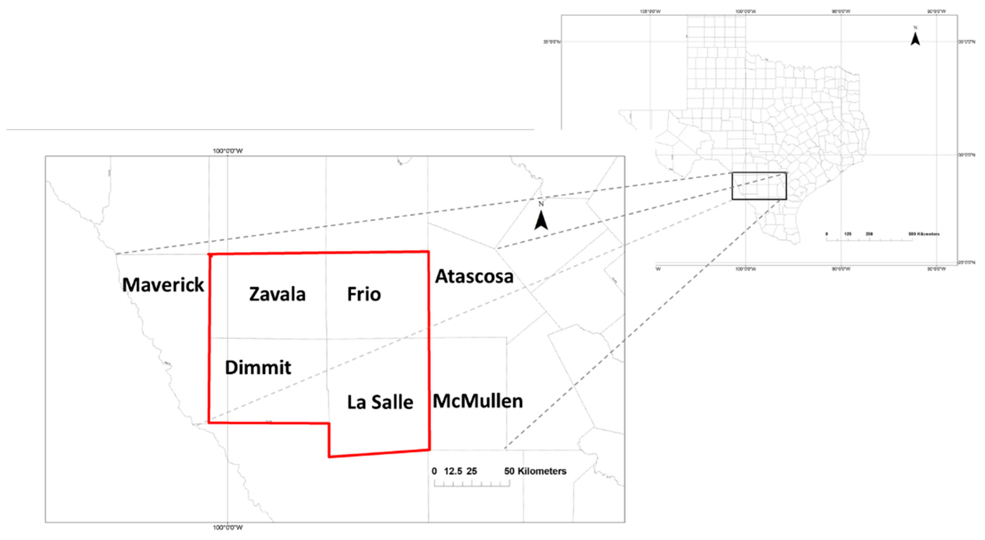
The Winter Garden Region of Texas (Figure 1) is noted for its year-round production of irrigated winter vegetables, and is among the leading producers in the U.S. Production is centered on four “core” counties—Dimmit, Frio, La Salle, and Zavala, but also includes parts of the Atascosa, Maverick, and McMullen counties [1]. The region grows a wide range of vegetable crops, including onions (Allium cepa L.), cabbage (Brassica oleracea. L.), spinach (Spinacia oleracea. L.), tomatoes (Solanum lycopersicum L.), beets (Beta procumbens), carrots (Daucus carota var. sativus), sweet potatoes (Ipomoea batatas), green beans (Phaseolus vulgaris L), potatoes (Solanum tuberosum L.), carrots (Daucus carota L.), pickling cucumbers (Cucumis sativus L.), greens (Brassica rapa subsp. rapa), and strawberries (Genus Fragaria L.). Other crops such as citrus fruits, melons, and nuts are also produced. Recently, vegetable production in the region has been facing a number of challenges. As is widely known, vegetable production is water intensive. For example, it takes 12.5 L of water to grow one tomato. Producers in the region utilize artesian aquifers, rivers, and reservoirs to provide water for irrigated crops. Droughts experienced in the past several years have reduced river water flows and caused some rivers to stop running. The Edwards, Carrizo-Wilcox, and other local aquifers are also low due to lack of adequate recharge and high irrigation water demands during the hot summer months. In addition to serious problems with insects and diseases, increased labor and inputs costs and competition from Mexico, especially after NAFTA was implemented, are affecting traditional market windows.
Despite these challenges, there is a tendency by producers to overirrigate to maintain target yields and quality. Such practices contribute to increased agricultural water demand, resulting in rising competition for water resources between agricultural and other sectors of the economy. Reduced freshwater availability for agriculture will need to be accompanied by improvements in water use efficiency. Improving water use efficiency in agriculture should be accompanied by increased efficiency of irrigation techniques. Irrigation efficiency can be defined as the effectiveness of the irrigation system in delivering all the water beneficially used to optimize crop production [2]. The effective use of water is influenced by the crops being irrigated, types of irrigation systems, and soil characteristics [2]. The irrigation system performance can be evaluated through the response of the crops to irrigation.
In this study, we proposed using the cropping system model ALMANAC (Agricultural Land Management Alternatives with Numerical Assessment Criteria) [3] that is capable of providing information on water requirements to grow vegetables. To optimize this cropping system model, data collected from field trials that were conducted on various vegetative types: common beans (Phaseolus vulgaris L.), green beans, cabbage, mint (Mentha), peppers (Capsicum annuum), and squash (Cucurbita), were used. The model was calibrated and validated using measured vegetable yields. The validated model was used to estimate various irrigation practices on vegetable yields and water use efficiency (WUE) in conceptually designed commercial irrigated plots in the Winter Garden Region under varying weather and with different soils. In addition, simulated water requirement results were used to calculate the economic feasibility of year-round vegetable production. The study results will provide recommendations to farmers for the best irrigation strategies for a range of different cropping management scenarios.
2. Materials and Methods
2.1. Description of Field Experiments
To develop key plant parameters for vegetables for the ALMANAC model, multiple field experimental plots were established at the USDA-ARS Grassland, Soil, and Water Research farm in Temple, TX, USA. Field experiments of beans, mint, pepper, squash, and cabbages were conducted in different years. The soil type at the site is a Houston Black clay (fine, montmorillonitic, thermic Udic Pellustert). Total precipitation and maximum and minimum temperature of the growing season of each vegetable are listed in Table 1. Supplemental irrigation was applied to ensure that the vegetable plants did not suffer any water stress. All plants were fertilized prior to planting by broadcasting 15–15–15 (nitrogen-phosphorus-potassium) fertilizer at 46 kg ha−1. Total aboveground biomass of all plants was harvested manually every two weeks throughout the growing season. At each harvest, the heights for all plants were measured from the ground to top of the highest leaf. Photosynthetically Active Radiation (PAR) was measured below the leaf canopy using an ACCUPAR LP-80 Ceptometer (Decagon Devices, Pullman, WA, USA). The PAR value was used to calculate the fraction of intercepted PAR (FIPAR). The light readings were made between 10:00 and 14:00. Fresh total aboveground biomass weight, seeds, and dead leaves were measured. The leaf area (cm2) for each plant sample was measured with a LI-3100 Area Meter (LI-COR Biosciences, Lincoln, NE, USA). Based on the leaf area, fresh weight, and sampling area, leaf area index (LAI) of each plant sample was calculated. The light extinction coefficient (k) was calculated as the natural log of difference between 1 and FIPAR and then divided by LAI. Following these measurements, the fresh samples were dried at 66 °C until dry weight stabilized, after which, the dry weights of each sample were measured. Detailed information on plot design, planting date, and harvesting date for each experiment is given below. The year and month of growing season of each vegetable are summarized in Table 1.
Study 1: In Study 1, one cultivar of bush beans and one cultivar of green beans were planted. In 2014, bush beans were planted at 90 kg per ha, two rows were 0.95 m apart with six to eight seeds per 0.3 m of row. Harvests were performed on September 25th, October 8th, October 24th, and November 4th. In 2016, green beans were planted at 90 kg per ha, in two rows 0.95 m apart at six to eight seeds per 0.3 m of row on May 1st. Harvests were done on May 25th, June 8th, June 21st, and July 7th.
Study 2: In 2015, cultivars of peppermint and spearmint were transplanted into plots on April 30th and May 15th, respectively. Four-week-old mint seedlings were purchased from the local feed store. Each plot consisted of three 3 m long rows, spaced 0.75 m apart, with 0.35 m between plants within rows, resulting in a plant density of 5.5. plants m−2. Harvests for each mint cultivar were done on May 6th, May25th, June 8th, June 21st, July 8th, and July 25th.
Study 3: In Study 3, cabbage (Brassica oleracea var. capitata) was planted as four-week-old cabbage seedlings purchased from a local feed store and transplanted into plots on October 1st, 2014. Each plot consisted of three 3 m long rows, spaced 0.75 m apart, with 0.35 m between plants within rows, resulting in a plant density of 5.5. plants m−2. Harvests were done on October 17th, October 31st, November 17th, December 5th, December 16th, and January 15th, 2015.
Study 4: In Study 4, two cultivars of squash, straight neck, and zucchini, were planted as four-week-old seedlings that were purchased from a local feed store and were transplanted into plots on June 15th, 2016. Plots consisted of three 3 m long rows of each of squash, spaced 0.75 m apart, with 0.35 m between plants within rows. Harvests were done on June 29th, July 5th, July 14th, July 21st, and July 25th for zucchini, while a total of eight harvests were done on June 29th, July 5th, July 14th, July 21st, July 25th, August 3rd, August 11th, and August 30th for straight neck.
Study 5: In Study 5, one cultivar of bell pepper was planted as four-week-old pepper seedlings that were purchased from a local feed store and transplanted into plots on June 1st, 2017. Each plot consisted of three 3 m long rows of each squash, spaced 0.75 m apart, with 0.35 m between plants within rows. Harvests were performed on June 13th, June 23rd, July 6th, July 18th, and July 26th.
2.2. Cropping Model Development
ALMANAC is a plant-oriented process-based model that simulates a large variety of crops and grasses. This model is sensitive to changes in soil properties, weather, and cropping management that affect water and nutrient supplies to plants. The model operates on a daily time step. The model simulates competition for light, water, and nutrients between plant species [4].
The model uses more than 50 plant parameters representative of various crops, grasses, shrubs, and trees. A set of parameters for each of the studied vegetables, including bush bean, green bean, peppermint, spearmint, cabbage, straight neck squash, zucchini, and bell pepper, were developed based on field measurements, literature reviews, and expert opinions. Based on the field measurements, some key parameters that include DLAI (fraction of growing season when leaf area index starts declining), DLAP1 (first point on optimal leaf area development curve), DLAP2 (second point on optimal leaf area development curve), HMX (maximum height, m), EXT (extinction coefficient for calculation of light interception), and HI (harvest index) were determined. The leaf area index can be used to calculate the vegetable crop growth rates. The calculated growth rates, DLAP1 and DLAP2, were used as plant parameters in the model (Table 2). TB (optimal temperature for plant growth) and TG (minimum temperature for plant growth) values were determined based on literature reviews. Other parameters were adapted from the ALMANAC plant database. The value of WA (energy to biomass conversion factor) and PHU (potential heat unit) were adjusted during the model calibration process. Some important key parameters for each vegetable are summarized in Table 2.
2.3. Model Validation
For each of the beans, squash, and pepper, the simulated either grain or fruit yield (dry Mg ha−1) was compared with the measured values from field trials in Temple, TX. For mint and cabbage, the simulated aboveground biomass dry yields (dry Mg ha−1) were compared with the measured values from the field trials in Temple. Model accuracy was tested by calculating RMSE (root mean square error) PB (percent bias) and R2 (coefficient of determination).
where i is the ith observation, n is the total number of observations, Si is the ith simulated value, Oi is ith observed value. Additionally, Pearson’s correlation coefficient of determination (R2) was estimated using Proc REG in Statistical Analysis Software version 9.3 (SAS 9.3).
2.4. Water Use Efficiency Changes in Various Irrigation Rates
After successful model yield validation, the simulated WUE was calculated for all vegetables. Two types of WUE, WUEwet and WUEdry, were calculated as wet or dry weight of plant yield or marketable yield divided by the quantity of plant transpiration during the growing season [5]. Since ALMANAC simulated dry weight of marketable yield, when we calculated WUEwet, the simulated yields were divided by (1 − (moisture content/100)). The moisture content was measured in each field trial. The measured moisture contents of bush beans, green bean, spearmint, peppermint, cabbage, zucchini, straight neck, and bell pepper were 88.0, 80.4, 58.2, 61.1, 87.4, 89.6, 90.3, and 87.1%, respectively.
2.5. Description of Study Irrigation Plots in Winter Garden Region in TX, USA
Eight irrigated locations were randomly selected from the Dimmit, La Salle, and Frio counties in the Winter Garden Region. All irrigated plots are classified as either Irrigated Capability Class 1 or 2, where soils have either no or moderate limitations that reduce the choice of plants or that require moderate conservation practices (NRCS-USDA, 2018). Soil types and their properties in the study locations are listed in Table A1. We developed and modeled 960 scenarios that represent projected vegetable production management conditions under different combinations of five irrigation rates, eight vegetable types, three years (2013, 2017, and 2019) and eight locations using the calibrated ALMANAC model. The five irrigation rates were 0, 50, 80, 100, and 150% of calculated crop evapotranspiration (ET) of each species in each study location. We used the same crop management that was used for model calibration and validation. The total rainfall amounts in mm during growing months in the Dimmit, La Salle, and Frio counites are listed in Table A2.
Based on the simulation results of 960 scenarios, analysis of variance (ANOVA) was used to statistically analyze the effects of treatment (irrigation regime) on the simulated marketable dry yield and water use efficiency (WUE). The Least Significant Difference test (LSD) was used to compare and rank the treatments. Simulated marketable dry yield under five irrigation rates (0, 50, 80, 100, and 150%) was analyzed for the eight vegetables. To accurately estimate monetary profit according to different water use, water cost was computed based on the water service fee in the Winter Garden Region of Texas [6]. Value creation rate (i.e., wet yield per water cost) was also analyzed. Logarithmic models were used to understand the trend of value creation rates of the eight vegetables. In addition, the profit of each vegetable was calculated by subtracting total irrigation water cost from revenue. The retail prices for bush bean, green bean, cabbage, yellow straight neck squash, zucchini, and bell pepper were obtained from USDA-Economic Research Service [7]. Spearmint and peppermint were excluded for profit analysis since their retail prices were not available from the USDA database. The revenue cost for each vegetable was obtained by multiplying total marketable wet yield with revenue cost. This study only considered water cost in order to understand precisely the impact of water use on vegetable profit.
3. Results and Discussion
3.1. Leaf Area Index and Yields of Eight Vegetable Crops
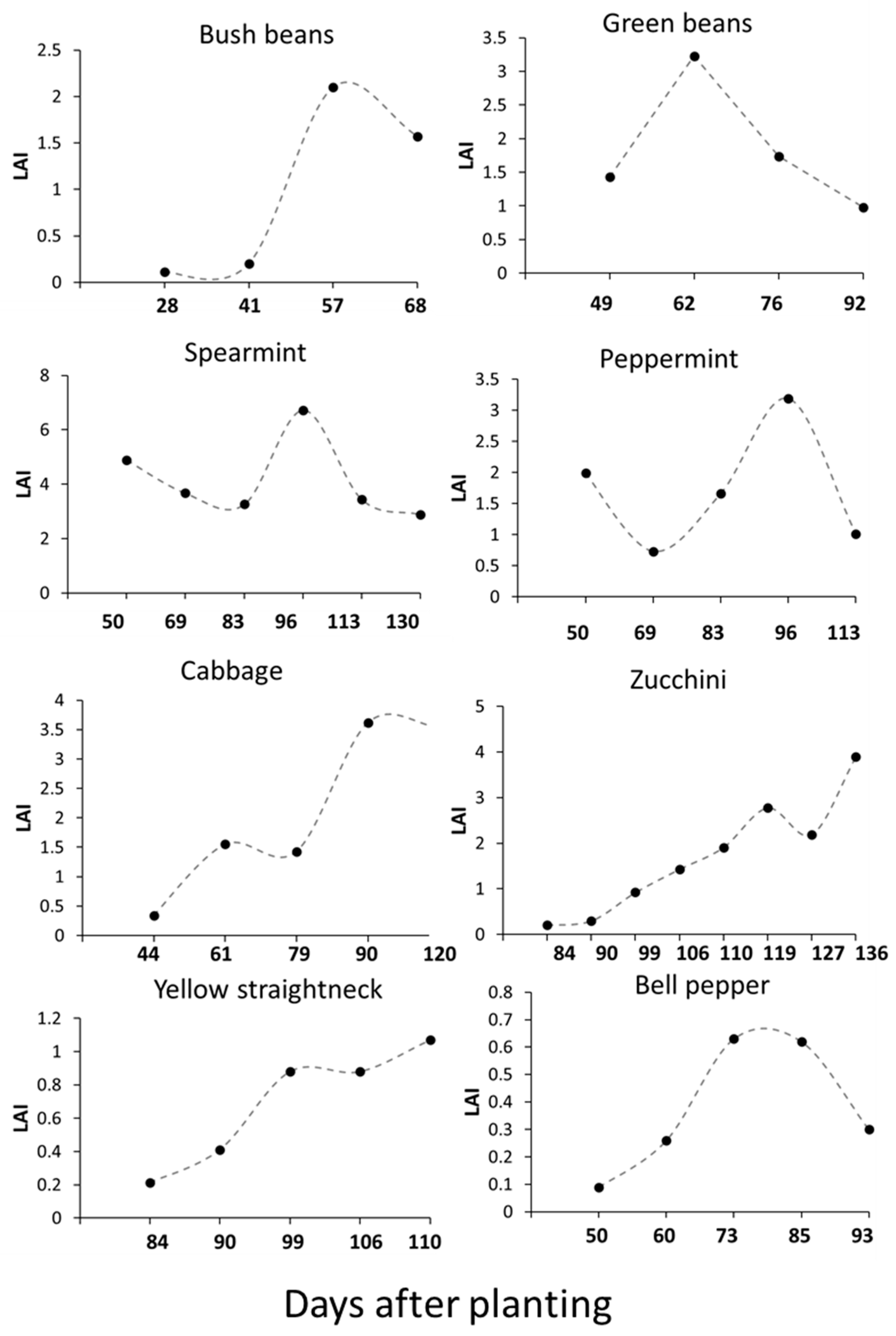
The eight vegetables had different growing days to approach maximum LAI in Temple, TX, USA (Figure 2). Among all vegetables, squash type plants had the longest growing days. Zucchini and yellow straight neck squash took 136 and 110 days, respectively, to approach their maximum LA (Figure 2). Both beans (bush bean and green bean) required at least 57–62 growing days to approach their maximum LAI. The two mints, cabbage, and bell pepper required at least 96, 96, 90, and 73 growing days to approach their maximum LAI, respectively. The value of maximum LAI varied among vegetables. Spearmint had the highest LAI, while bell pepper had the lowest among the vegetables.
3.2. ALMANAC Yield and Water Use Efficiency Simulation and Validation
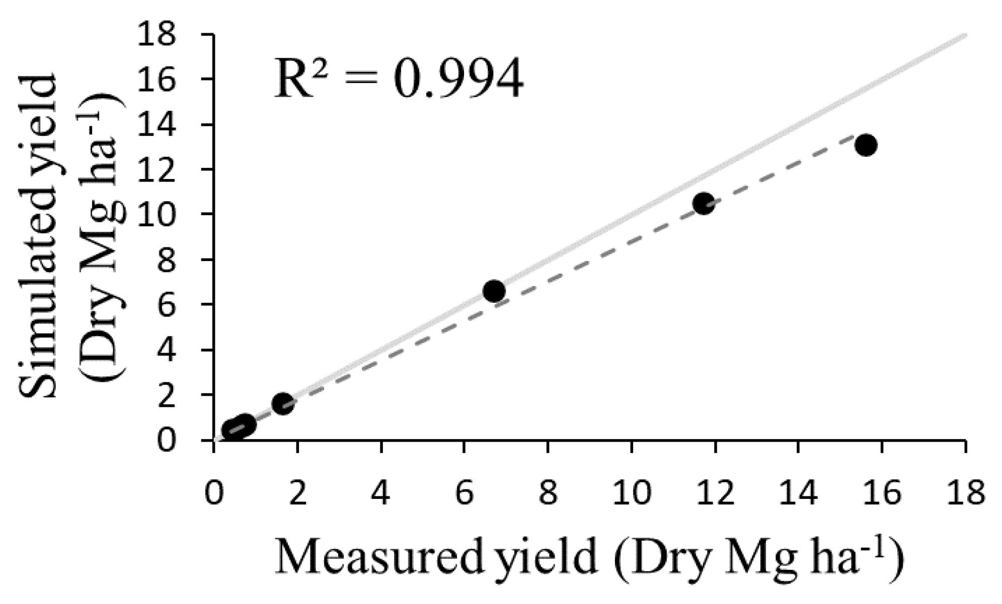
ALMANAC simulated marketable yields of all the vegetables, except spearmint, agreed well with the measured yields (Table 3 and Figure 3). The simulated and measured yields were compared using RMSE, PBIAS, and R2. The value of RMSE was 0.97 Mg ha−1, and the PBIAS was only 9.4%. The value of R2 was 0.99 as shown in Figure 3. ALMANAC’s simulated yield of spearmint underestimated the measured yield by 2.5 Mg ha−1 (Table 3).
Water use efficiency (WUE) values for all eight vegetables were calculated based on the simulation results. Since ALMANAC simulated the dry yields, moisture contents were multiplied to the yields, and the results were divided by the amount of water that was transpired by the plants during the growing season. In general, the simulated WUEs were moderately close to the values in range of the measured WUE reported by [8,9,10,11,12,13] (Table 4). Among all eight vegetables, cabbage had the highest WUE, while zucchini had the lowest WUE.
As shown in the results, ALMANAC accurately simulated yields of all eight vegetables. Although a limited number of years of data was used to develop each crop model, the model also could realistically simulate WUE when we compared the simulated WUE values with references. Thus, we assumed that ALMANAC model has been successfully validated. Following the successful validation of the ALMANAC model, we applied the model to predict vegetable production in the Winter Garden Region, and simulation results were used for production economic analysis.
3.3. Vegetable Yield Predictions and Water Use Efficiency in Winter Garden Region in TX, USA
In general, the marketable simulated yields for bush bean, green bean, spearmint, peppermint, cabbage, and yellow straight neck squash increased with increasing amounts of irrigation water (Table 5). The lowest yields for these vegetables were obtained under no irrigation treatment. Bush bean, green bean, spearmint, and peppermint had the highest yields at 150% of ET. Bush bean showed no significant yield differences between 50 and 100% of ET. Spearmint and peppermint showed no significant yield difference between 80 and 100% of ET. Yields for cabbage and yellow straight neck squash did not differ from 50% to 150% of ET and from 100 to 150% of ET, respectively. The marketable yields for zucchini and bell pepper did not significantly differ from 0 to 150% of ET (Table 5).
For most vegetables, there were no significant effects of irrigation treatments on WUE (Table 5). For green bean and zucchini, WUE decreased with increasing irrigation amount. The highest values of WUE were obtained under either no irrigation or low irrigation treatment, while the lowest WUE values were observed at 150% of ET.
3.4. Optimization of Irrigation Water Use Efficiency in Winter Garden Region in TX, USA
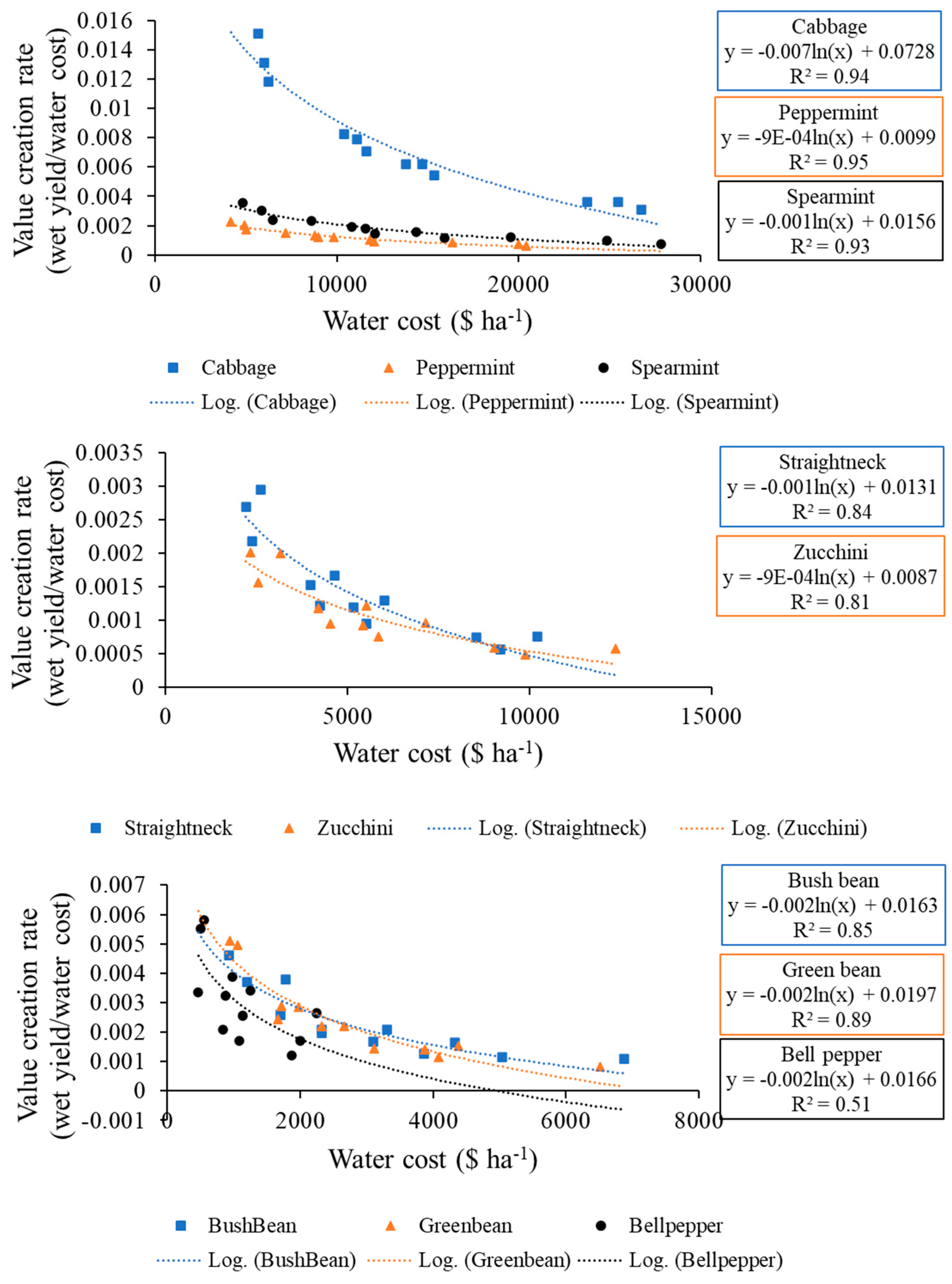
The value creation rates (i.e., yield per water cost) of all eight vegetables were compared (Figure 4). The rates in Figure 4 show how WUE affects the yield of each vegetable. The eight vegetables were classified in three groups according to their water use: (1) High (0–1600 m3/ha), (2) Medium (0–900 m3/ha), and (3) Low (0–600 m3/ha). The High group included cabbage, peppermint, and spearmint, and had higher value creation rates than other vegetables. For example, if a farmer spends $5000 per ha, the farmer can get about 4 Mg ha−1 of spearmint. However, the same amount of water cost, he can only produce 0.52 Mg ha−1 of zucchini and 0.75 Mg ha−1 of green bean. The Medium group includes yellow straight neck squash and zucchini, while the Low group includes green bean, bush bean, and bell pepper. Although the vegetables had different value creation rates, their patterns were similar. This is because the vegetable yields did not change much after certain amounts of water had been applied (Table 5). To be more specific, the yield of the High group became stable after 600 m3 ha−1 water supplied. Similarly, the yields of the Medium group and the Low group became stable after 200 m3 ha−1 and 100 m3 ha−1 water supplied, respectively. In other words, once there is sufficient water supply at a farm, a farmer does not have to spend his/her money for more water.
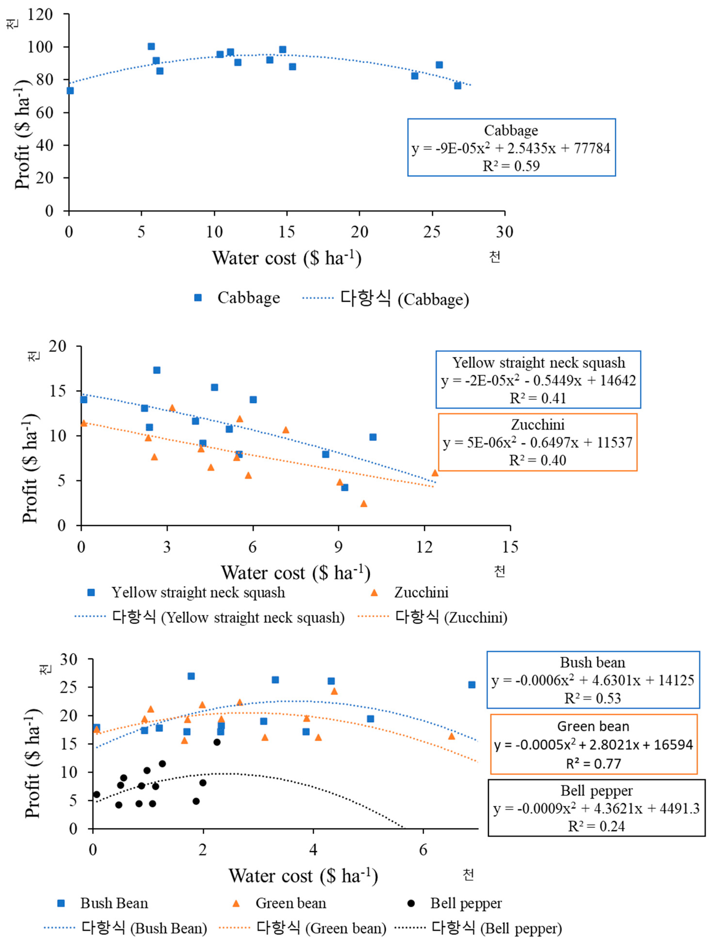
The value creation rates shown in Figure 4 are directly related to profit of each vegetable. The profit of vegetables tends to have a concave function according to water cost. Initially, the profit increases as total irrigation water cost increased. However, once there is a low value creation rate, the profit decreases as total irrigation water cost increased. This is because vegetable yield does not significantly increase after a certain amount of water used (see Figure 4). In Figure 5, the total profit of cabbage decreases after $14,000 of water cost (i.e., 960 m3 ha−1 of water use). Similarly, the total profits of bush bean, green bean, and bell pepper can be maximized at water cost of $3600 (322 m3 ha−1 of water use), $2200 (219 m3 ha−1 of water use), and $2600 (248 m3 ha−1 of water use), respectively. Unlike other vegetables, yellow straight neck squash and zucchini have a negative relationship between profit and water cost. In fact, the percentage of water cost from revenue is 30.81% for yellow straight neck squash and 39.63% for zucchini. Considering that the percentages of other vegetables are less than 13%, the water cost is too expensive for both vegetables. The highest profits of yellow straight neck squash and zucchini were obtained when there is no irrigation (i.e., rainfall only). As a result, appropriate amounts of water should be used to maximize profit of each vegetable.
Frequent and more severe droughts, limited water resources, and increased regulations restricting water use are major constraints to vegetable production in the Winter Garden Region in TX. With the increased costs of irrigation, vegetable production acreage has continuously decreased. However, the Winter Garden counties are still among the leading producers of winter vegetables through irrigation in TX. Climate change and Covid-19 pandemic (a global health crisis) pose some serious challenges in twenty-first century agriculture worldwide. For sustainable vegetable production systems for food and nutrition security, it is critical to find solutions or cropping strategies that provide high-quality, attractive, and nutritious vegetables under limited water conditions. The results presented in this paper are useful guides for the best selection of irrigation strategies that maximize vegetable yields and economic benefits to farmers. The ALMANAC simulation model can be extremely valuable as a research tool that provides useful recommendations for decision-making processes based on the maximization of annualized net returns to farmers.
4. Conclusions
Reduced freshwater availability for agriculture necessitates greater efficiency of irrigation techniques. However, this increased irrigation efficiency should not compromise crop quality, yields, and farmer’s profits. An efficient systems approach and decision support tools that are specifically designed for the analyses of agricultural and economic impacts of applying various irrigation amounts to common vegetable crops under different weather and soil conditions could assist producers in establishing guidelines for the efficient use of irrigation. In the present study, field trials were conducted on eight vegetables (bush bean, green bean, cabbage, peppermint, spearmint, yellow straight neck squash, zucchini, and bell pepper). The field data were used to develop the vegetable model parameters. The ALMANAC model was validated with the measured values, and the model successfully simulated the eight vegetable yields (R2 = 0.99). The developed model was used to simulate 960 scenarios compromised of different conditions for eight locations, eight vegetable types, and five irrigation regimes (0, 50, 80, 100, and 150% of calculated each vegetable evapotranspiration) over 3 years. Based on the simulation results, the impacts of various irrigation application amounts on the yields and WUE were evaluated. In general, and as expected, the vegetable yields increased as irrigation amount increased. However, the vegetable yields were not largely increased after a certain irrigation level. Therefore, farmer’s profit from vegetables decreased as the total irrigation water cost increased. Since the sufficient irrigation water amount that comprises crop yield and farmer’s profit differed by vegetable type, this vegetable modeling framework can be used to provide useful information to farmers regarding appropriate amounts of irrigation water used for various vegetable types.
Author Contributions
Conceptualization, S.K. (Sumin Kim), M.N.M., and S.K. (Sojung Kim); Methodology, S.K. (Sumin Kim) and S.K. (Sojung Kim); Software, S.K. (Sumin Kim) and S.K. (Sojung Kim); Validation, S.K. (Sumin Kim); Formal Analysis, S.K. (Sumin Kim) and S.K. (Sojung Kim); Investigation, S.K. (Sumin Kim) and S.K. (Sojung Kim); Resources, S.K. (Sumin Kim); Writing–Original Draft Preparation, S.K. (Sumin Kim), M.N.M., and S.K. (Sojung Kim); Writing–Review and Editing, S.K. (Sumin Kim), M.N.M., and J.R.K.; Visualization, S.K. (Sumin Kim) and S.K. (Sojung Kim); Project Administration, J.R.K.; Funding Acquisition, J.R.K. All authors have read and agreed to the published version of the manuscript.
Funding
This work was also supported in part by an appointment to the Agricultural Research Service administered by the Oak Ridge Institute for Science and Education through interagency agreement between the U.S. Department of Energy (DOE) and the U.S. Department of Agriculture (USDA), Agricultural Research Service Agreement #60-3098-5-002. This work was supported by the Dongguk University Research Fund of 2020.
Acknowledgments
We are grateful to Amber S. Williams and Greeson Ricky for their valuable support of this research. This work was supported by the Dongguk University Research Fund of 2020.
Conflicts of Interest
The authors declare no conflict of interest.
Appendix A

Table A1.
Soil types and properties in study locations in Dimmit, La Salle, and Frio Counties, TX, U.S.
Table A1.
Soil types and properties in study locations in Dimmit, La Salle, and Frio Counties, TX, U.S.
| County | Simulation Location | Soil Types | Soil Properties (%) | |||
|---|---|---|---|---|---|---|
| Latitude | Longitude | Sand | Silt | Clay | ||
| Dimmit | 28.98757 | −99.8461 | Uvalde clay loam | 25 | 41 | 34 |
| Dimmit | 28.99945 | −99.8447 | Bookout clay loam | 29 | 40 | 31 |
| Frio | 28.76791 | −99.0803 | Duval loamy fine sand | 85 | 6 | 9 |
| Frio | 28.85791 | −99.1274 | Duval loamy fine sand | 85 | 6 | 9 |
| Frio | 28.77793 | −99.091 | Duval loamy fine sand | 85 | 6 | 9 |
| Frio | 28.82222 | −99.0627 | Duval loamy fine sand | 85 | 6 | 9 |
| LaSalle | 28.51857 | −98.8769 | Caid very fine sandy loam | 63 | 24 | 13 |
| LaSalle | 28.53059 | −99.2402 | Duval very fine sandy loam | 78 | 9 | 13 |
Table A2.
Total rainfall during growing months for all 8 vegetables in Dimmit, La Salle, and Frio Counties in TX, U.S. BB: bush bean; GB: green bean; SM: spearmint; PP: peppermint; C: cabbage; Z: zucchini; S: yellow straight neck squash; BP: bell pepper.
Table A2.
Total rainfall during growing months for all 8 vegetables in Dimmit, La Salle, and Frio Counties in TX, U.S. BB: bush bean; GB: green bean; SM: spearmint; PP: peppermint; C: cabbage; Z: zucchini; S: yellow straight neck squash; BP: bell pepper.
| BB | GB | SM | PP | C | Z | S | BP | |
|---|---|---|---|---|---|---|---|---|
| Growing months | 8~10 | 4~6 | 10~2 | 10~2 | 8~12 | 4~8 | 4~8 | 4~7 |
| Dimmit | ||||||||
| 2013 | 409.7 | 276.1 | 378.1 | 378.1 | 435.3 | 280.4 | 280.4 | 276.1 |
| 2017 | 244.6 | 124.1 | 165.7 | 165.7 | 344.3 | 156.1 | 156.1 | 124.1 |
| 2019 | 61.6 | 134.2 | 144.6 | 144.6 | 62.9 | 140 | 140 | 134.2 |
| Frio | ||||||||
| 2013 | 233 | 121.1 | 111 | 111 | 246.9 | 168 | 168 | 121.1 |
| 2017 | 245.4 | 150.8 | 72.1 | 72.1 | 282.3 | 257.8 | 257.8 | 150.8 |
| 2019 | 206.74 | 233.9 | 122.7 | 122.7 | 249.94 | 293.04 | 293.04 | 233.9 |
| La Salle | ||||||||
| 2013 | 297.4 | 159.7 | 279.9 | 279.9 | 320.1 | 166.1 | 166.1 | 159.7 |
| 2017 | 217 | 171.1 | 89.9 | 89.9 | 278.5 | 235.9 | 235.9 | 171.1 |
| 2019 | 206.74 | 233.9 | 122.7 | 122.7 | 249.94 | 293.04 | 293.04 | 233.9 |
References
- Odintz, M. Winter Garden Region. In Handbook of Texas Online; Texas State Historical Association: Austin, TX, USA, 2019. [Google Scholar]
- Irmak, S.; Odhiambo, L.O.; Kranz, W.L.; Eisenhauer, D.E. Irrigation Efficiency and Uniformity, and Crop Water Use Efficiency. Biol. Syst. Eng. Pap. Publ. 2011, 451, 1–8. [Google Scholar]
- Kiniry, J.R.; Arnold, J.G.; Xie, Y. Applications of Models with Different Spatial Scales. In Agricultural System Models in Field Research and Technology Transfer; Ahuja, L.R., Ma, L., Howell, T.A., Eds.; CRC Press: Boca Rotan, FL, USA, 2002; pp. 207–227. [Google Scholar]
- Williams, J.R.; Arnold, J.G.; Kiniry, J.R.; Gassman, P.W.; Green, C.H. History of model development at Temple, Texas. Hydrol. Sci. J. 2008, 53, 948–960. [Google Scholar] [CrossRef] [Green Version]
- Kim, S.; Kim, S.; Cho, J.; Park, S.; Jarrín Perez, F.X.; Kiniry, J.R. Simulated Biomass, Climate Change Impacts, and Nitrogen Management to Achieve Switchgrass Biofuel Production at Diverse Sites in U.S. Agronomy 2020, 10, 503. [Google Scholar] [CrossRef] [Green Version]
- System, S.A.W. Landscape Irrigation Service Rates. Available online: https://www.saws.org/service/water-sewer-rates/landscape-irrigation-service-rates/ (accessed on 15 July 2020).
- USDA-ERS. Fruit and Vegetable Prices. Available online: https://www.ers.usda.gov/data-products/fruit-and-vegetable-prices/fruit-and-vegetable-prices/#Vegetables (accessed on 15 July 2020).
- El-Noemani, A.A.; El-Zeiny, H.A.; El-Gindy, A.M.; El-Sahhar, E.A.; El-Shawadfy, M.A. Performance of Some Bean (Phaseolus vulgaris L.) Varieties under Different Irrigation Systems and Regimes. Aust. J. Basic Appl. Sci. 2010, 4, 6185–6196. [Google Scholar]
- Saleh, S.; Liu, G.; Liu, M.; Ji, Y.; He, H.; Gruda, N. Effect of Irrigation on Growth, Yield, and Chemical Composition of Two Green Bean Cultivars. Horticulturae 2018, 4, 3. [Google Scholar] [CrossRef] [Green Version]
- O. Elansary, H.; Mahmoud, E.A.; El-Ansary, D.O.; Mattar, M.A. Effects of Water Stress and Modern Biostimulants on Growth and Quality Characteristics of Mint. Agronomy 2020, 10, 6. [Google Scholar] [CrossRef] [Green Version]
- Jangandi, S.; Shekar, B.; Sridhara, S. Water use efficiency and yield of cabbage as influenced by drip and furrow methods of irrigation. Indian Agric. 2001, 44, 153–155. [Google Scholar]
- Rouphael, Y.; Colla, G.; Battistelli, A.; Moscatello, S.; Proietti, S.; Rea, E. Yield, water requirement, nutrient uptake and fruit quality of zucchini squash grown in soil and closed soilless culture. J. Hortic. Sci. Biotechnol. 2004, 79, 423–430. [Google Scholar] [CrossRef]
- Shammout, M.W.; Qtaishat, T.; Rawabdeh, H.; Shatanawi, M. Improving Water Use Efficiency under Deficit Irrigation in the Jordan Valley. Sustainability 2018, 10, 4317. [Google Scholar] [CrossRef] [Green Version]
Figure 1.
Map of the Winter Garden Region in Texas including all of the Dimmit, La Salle, Zavala, and Frio counties, and portions of the Maverick, Atascosa, and McMullen counties. The red line indicates the four leading irrigated vegetable-growing counties.
Figure 1.
Map of the Winter Garden Region in Texas including all of the Dimmit, La Salle, Zavala, and Frio counties, and portions of the Maverick, Atascosa, and McMullen counties. The red line indicates the four leading irrigated vegetable-growing counties.

Figure 2.
Measured leaf area index (LAI) of eight vegetables planted in Temple, TX, USA.

Figure 3.
Relationship between measured and ALMANAC-simulated dry marketable yields of vegetables grown in Temple, TX. The dashed line is the fitted regression line and solid line is the 1:1 line.
Figure 3.
Relationship between measured and ALMANAC-simulated dry marketable yields of vegetables grown in Temple, TX. The dashed line is the fitted regression line and solid line is the 1:1 line.

Figure 4.
Value creation rates (i.e., marketable wet yield per water cost) of all 8 vegetables grown in the Winter Garden Region under four irrigation regimes (50, 80, 100, and 150% of ET).
Figure 4.
Value creation rates (i.e., marketable wet yield per water cost) of all 8 vegetables grown in the Winter Garden Region under four irrigation regimes (50, 80, 100, and 150% of ET).

Figure 5.
Comparison of farmer’s profit with total cost of irrigation when 6 vegetables were grown in several locations in Winter Garden Region in TX, USA under five irrigation regimes (0, 50, 80, 100, and 150% of ET).
Figure 5.
Comparison of farmer’s profit with total cost of irrigation when 6 vegetables were grown in several locations in Winter Garden Region in TX, USA under five irrigation regimes (0, 50, 80, 100, and 150% of ET).

Table 1.
Year, months, total precipitation, maximum temperature, and minimum temperature of the growing season of each vegetable planted in Temple, TX, USA.
Table 1.
Year, months, total precipitation, maximum temperature, and minimum temperature of the growing season of each vegetable planted in Temple, TX, USA.
| Vegetables | Year of Growing Season | Months of Growing Season | Growing Season | ||
|---|---|---|---|---|---|
| Total | Maximum | Minimum | |||
| Precipitation (mm) | Temp. (°C) | Temp. (°C) | |||
| Bush bean | 2014 | Aug.–Nov. | 263 | 31.7 | 19.8 |
| Green bean | 2016 | April–June | 434 | 28.1 | 18.1 |
| Peppermint | 2015 | April–June | 434 | 28.1 | 18.1 |
| Spearmint | 2015 | April–June | 434 | 28.1 | 18.1 |
| Cabbage | 2014–2015 | Aug.–Jan. | 537 | 23.6 | 12.6 |
| Straight neck | 2016 | April–Aug. | 651 | 30.6 | 20.2 |
| Zucchini | 2016 | April–July | 451 | 30.1 | 19.6 |
| Bell pepper | 2017 | April–July | 385 | 30.7 | 19.1 |
Table 2.
Key parameters of each vegetable used in ALMANAC model calibration.
| Key Parameters | Vegetables | |||||||
|---|---|---|---|---|---|---|---|---|
| Bush Bean | Green Bean | Pepper Mint | Spearmint | Cabbagge | Straight Neck | Zucchini | Bell Pepper | |
| WA | 25 | 30 | 30 | 40 | 40 | 25 | 25 | 30 |
| HI | 0.4 | 0.45 | 0.001 | 0.001 | 0.2 | 0.64 | 0.22 | 0.57 |
| TB | 30 | 30 | 25 | 25 | 19 | 25 | 25 | 30 |
| TG | 8 | 8 | 12 | 12 | 0 | 15 | 15 | 12.8 |
| DLAI | 0.75 | 0.5 | 0.5 | 0.5 | 0.9 | 0.75 | 0.75 | 0.76 |
| DLAP1 | 58.05 | 42.44 | 40.22 | 40.55 | 34.09 | 73.20 | 59.09 | 49.14 |
| DLAP2 | 89.99 | 54.99 | 85.99 | 62.99 | 78.99 | 95.82 | 86.71 | 76.99 |
| HMX | 0.44 | 0.44 | 0.33 | 1 | 0.33 | 0.55 | 0.58 | 1 |
| EXT | 0.45 | 0.46 | 0.4 | 0.4 | 0.46 | 0.45 | 0.45 | 1.27 |
Table 3.
Measured and ALMANAC-simulated marketable yields of 8 vegetables grown in Temple, TX.
| Vegetables | Yield Type | Measured Yield | Simulated Yield |
|---|---|---|---|
| Dry Mg ha−1 | Dry Mg ha−1 | ||
| Bush bean | Pod | 0.66 | 0.67 |
| Green bean | Pod | 1.64 | 1.65 |
| Pepper mint | Above-ground biomass | 6.7 | 6.67 |
| Spearmint | Above-ground biomass | 15.6 | 13.12 |
| Cabbage | Above-ground biomass | 11.7 | 10.55 |
| Yellow straight neck | Squash | 0.50 | 0.51 |
| Zucchini | Squash | 0.41 | 0.46 |
| Bell pepper | Pepper | 0.71 | 0.73 |
| RMSE | 0.97 | ||
| PBIAS | 9.4 |
Table 4.
Measured moisture contents, ALMANAC-simulated Water Use Efficiency (WUE) for either wet or dry yield basis, and measured WUE reported in the literature.
Table 4.
Measured moisture contents, ALMANAC-simulated Water Use Efficiency (WUE) for either wet or dry yield basis, and measured WUE reported in the literature.
| Vegetables | Measured | Simulated | Reported | Reference | ||
|---|---|---|---|---|---|---|
| Moisture | WUEwet | WUEdry | WUEwet | WUEdry | ||
| Content (%) | mg g−1 | mg g−1 | mg g−1 | mg g−1 | ||
| Bush bean | 88.0 | 5.5 | 0.7 | 1–4.5 | - | [8] |
| Green bean | 80.4 | 7.4 | 1.4 | 4.3–6.3 | - | [9] |
| Spearmint | 58.2 | 5.7 | 2.4 | 1.9–2.8 | - | [10] |
| Peppermint | 61.1 | 4.0 | 1.5 | 1.9–2.8 | - | [10] |
| Cabbage | 87.4 | 31.8 | 4.0 | 27.9–54.1 | - | [11] |
| Yellow straight neck squash | 89.6 | 4.3 | 0.4 | - | - | N.A. |
| Zucchini | 90.3 | 2.9 | 0.3 | - | 0.7–1.4 | [12] |
| Bell pepper | 87.1 | 12.2 | 1.6 | 9.3–10.8 | - | [13] |
Table 5.
Simulated marketable dry yields (Mg ha−1) and water use efficiency (WUEwet) for 8 vegetables grown under different irrigation regimes in the Winter Garden Region in TX, USA. Yield and WUE with same letters are not significantly different (p < 0.05) within each vegetable type (ANOVA, LSD).
Table 5.
Simulated marketable dry yields (Mg ha−1) and water use efficiency (WUEwet) for 8 vegetables grown under different irrigation regimes in the Winter Garden Region in TX, USA. Yield and WUE with same letters are not significantly different (p < 0.05) within each vegetable type (ANOVA, LSD).
| Vegetables | Irrigation Regimes | Yield | WUEwet | Vegetables | Yield | WUEwet | Vegetables | Yield | WUEwet | ||
|---|---|---|---|---|---|---|---|---|---|---|---|
| Bush bean | 0 | 0.51 c | 5.8 | Peppermint | 0 | 2.7 c | 15 | Zucchini | 0 | 0.57 | 4.2 ab |
| 50 | 0.62 ab | 6.3 | 50 | 3.7 bc | 14 | 50 | 0.65 | 4.5 a | |||
| 80 | 0.65 ab | 6.4 | 80 | 4.3 ab | 14 | 80 | 0.66 | 4.4 ab | |||
| 100 | 0.68 ab | 6.4 | 100 | 4.6 ab | 14 | 100 | 0.66 | 4.4 ab | |||
| 150 | 0.73 a | 6.6 | 150 | 5.25 a | 15 | 150 | 0.67 | 3.8 b | |||
| p-value | 0.04 | n.s. | p-value | <0.0001 | n.s. | p-value | n.s. | 0.04 | |||
| Green bean | 0 | 0.81 c | 8.7 a | Cabbage | 0 | 7.46 b | 32 | Bell pepper | 0 | 0.27 | 6.6 |
| 50 | 0.92 bc | 8.4 ab | 50 | 10 a | 34 | 50 | 0.32 | 7.1 | |||
| 80 | 0.99 b | 8.3 ab | 80 | 10.7 a | 34 | 80 | 0.36 | 7.3 | |||
| 100 | 1.03 ab | 8.2 ab | 100 | 10.9 a | 35 | 100 | 0.39 | 7.6 | |||
| 150 | 1.15 a | 7.3 b | 150 | 11 a | 30 | 150 | 0.5 | 6.5 | |||
| p-value | <0.00001 | 0.031 | p-value | <0.0001 | n.s. | p-value | n.s. | n.s. | |||
| Spearmint | 0 | 4.9 c | 23 | Yellow straight neck squash | 0 | 0.43 b | 2.9 | ||||
| 50 | 7 bc | 23 | 50 | 0.48 ab | 2.9 | ||||||
| 80 | 8.1 ab | 21 | 80 | 0.52 ab | 2.8 | ||||||
| 100 | 8.6 ab | 20 | 100 | 0.53 a | 2.8 | ||||||
| 150 | 9.6 a | 18 | 150 | 0.56 a | 2.7 | ||||||
| p-value | <0.0001 | n.s. | p-value | 0.007 | n.s. |
© 2020 by the authors. Licensee MDPI, Basel, Switzerland. This article is an open access article distributed under the terms and conditions of the Creative Commons Attribution (CC BY) license (http://creativecommons.org/licenses/by/4.0/).
Share and Cite
MDPI and ACS Style
Kim, S.; Meki, M.N.; Kim, S.; Kiniry, J.R. Crop Modeling Application to Improve Irrigation Efficiency in Year-Round Vegetable Production in the Texas Winter Garden Region. Agronomy 2020, 10, 1525. https://doi.org/10.3390/agronomy10101525
AMA Style
Kim S, Meki MN, Kim S, Kiniry JR. Crop Modeling Application to Improve Irrigation Efficiency in Year-Round Vegetable Production in the Texas Winter Garden Region. Agronomy. 2020; 10(10):1525. https://doi.org/10.3390/agronomy10101525
Chicago/Turabian StyleKim, Sumin, Manyowa N. Meki, Sojung Kim, and James R. Kiniry. 2020. "Crop Modeling Application to Improve Irrigation Efficiency in Year-Round Vegetable Production in the Texas Winter Garden Region" Agronomy 10, no. 10: 1525. https://doi.org/10.3390/agronomy10101525
Note that from the first issue of 2016, this journal uses article numbers instead of page numbers. See further details here.