A Simple Light-Use-Efficiency Model to Estimate Wheat Yield in the Semi-Arid Areas

Abstract

In this study, a simple model, based on a light-use-efficiency model, was developed in order to estimate growth and yield of the irrigated winter wheat under semi-arid conditions. The originality of the proposed method consists in (1) the modifying of the expression of the conversion coefficient (ε_conv) by integrating an appropriate stress threshold (k_sconv) for triggering irrigation, (2) the substitution of the product of the two maximum coefficients of interception (ε_imax) and conversion (ε_{conv_max}) by a single parameter ε_max, (3) the modeling of ε_max as a function of the Cumulative Growing Degree Days (CGDD) since sowing date, and (4) the dynamic expression of the harvest index (HI) as a function of the CGDD and the final harvest index (HI₀) depending on the maximum value of the Normalized Difference Vegetation Index (NDVI). The calibration and validation of the proposed model were performed based on the observations of wheat dry matter (DM) and grain yield (GY) which were collected on the R3 irrigated district of the Haouz plain (center of Morocco), during three agricultural seasons. Further, the outputs of the simple model were also evaluated against the AquaCrop model estimates. The model calibration allowed the parameterization of ε_max in four periods according to the wheat phenological stages. By contrast, a linear evolution was sufficient to represent the relationship between HI and CGDD. For the model validation, the obtained results showed a good agreement between the estimated and observed values with a Root Mean Square Error (RMSE) of about 1.07 and 0.57 t/ha for DM and GY, respectively. These correspond to a relative RMSE of about 19% for DM and 20% for GY. Likewise, although of its simplicity, the accuracy of the proposed model seems to be comparable to that of the AquaCrop model. For GY, R², and RMSE values were respectively 0.71 and 0.44 t/ha for the developed approach and 0.88 and 0.37 t/ha for AquaCrop. Thus, the proposed simple light-use-efficiency model can be considered as a useful tool to correctly reproduce DM and GY values.

1. Introduction

In the southern Mediterranean area, drought is increasing in frequency and intensity [1]. Associated with global climate change, this trend will likely be more evident in the future [2]. Drought damage to the agricultural sector affects both rural livelihoods and the national economy as a whole.

Morocco is an arid and semi-arid regions where water resources are very limited [3,4], and characterized by a high sensitivity to climatic conditions [5]. In this region, cereals are the dominant crop at the national scale [6]. With a high evaporative demand (about 1600 mm/year), frequent irrigation is crucially needed to reach potential growth and yield [7]. Indeed, about 85% of total annual water consumption is used for agriculture irrigation in the region [4]. In this context, accurate and real-time estimation of crop yield at different scales (e.g., local, regional, or national) is becoming increasingly important [8]. Additionally, rapid and precise acquisition of field information (e.g., land use, water status, and crop phenological stages) and crop production is important for formulating agricultural development planning and agricultural policy [9]. More specifically, to preserve water resources, the rational management of irrigation water is necessary [10,11].

Modelling can be a useful tool to assess and develop promising irrigation scheduling strategies under limited available water for increasing crop water productivity [12]. The challenge is to link meteorological conditions, soil properties, and field management controlling crop production, in order to better describe the processes leading to crop biomass and yield. In this context, crop modeling is an effective way to simulate the mechanisms and semi-empirical procedures associated to crop growth [13,14,15]. Many process-based crop models have been developed [16], such as AquaCrop [17], STICS [18], DSSAT [19], APSIM [20], SUCROS87 [21], WOFOST [22], and CERES [23]. Nevertheless, a common challenge for using these models is the necessity of knowing several input parameters describing the agro-environmental conditions, which are not always available. The diversities of wheat cultivars, water and fertilizer management, pests and diseases control, and field application (e.g., mulching) in most farmlands have greatly limited the application of such crop models at local and large-scale regions [13,14,24]. Thus, these models are used principally by scientists or engineers for academic research and cannot be used on a daily basis by actual field managers [25,26]. To address this issue, two types of models have been used. The first are the empirical models linking a vegetation index observed by remote sensing (like Normalised Difference Vegetation Index, NDVI), at a given time, to the final biomass and grain yield [27,28,29,30,31]. This kind of relationship is simple to develop but remains very sensitive to agro-environmental conditions and varies from one agricultural season to the other [29]. In addition, this approach integrates the effects of all types of stress into the vegetation index, which limits its use to drive the crop management and/or to interpret the crop yields [30,32]. The second alternative, which is based on light-use-efficiency [33], provides great potential for plant biomass estimation. This approach was implemented in several models such as CASA [24], LINTUL [34], and GLO-PEM [35]. In these models, biomass accumulation is transformed from the effective radiation intercepted by the crop canopy. Most of these models were widely used to estimate net primary productivity on either grassland or forest by using remote sensing data [36,37,38], but not as much for crops, because of less interpretation of processes of crop growth and field management [32]. Then, these models need to couple the light-use-efficiency theory with biomass partitioning [39], to simulate growth process and estimate yield for herbaceous crops. In real conditions, the climatic and soil conditions can modify the temporal evolution of the conversion efficiency [32]. Any stress having an influence on the stomata opening leads to a decrease in crop transpiration, thus a decrease in photosynthetic activity which results to a reduction in the conversion efficiency [32]. The most important external factors that can cause this closure of the stomata are water content, nitrogen content, and temperature.

This study proposes an enhancement of the Monteith light-use-efficiency model [33], to estimate wheat production in semi-arid areas. More specifically, stress factors introduced by the shortage of water and temperature will be expressed in a conversion coefficient of light intercepted to the biomass. The manuscript is organized as follows: Section 2 provides a description of the study area, in-situ measurements and satellite imagery, and the proposed approach to estimate wheat production. Section 3 presents the results and discussions about model calibration and validation. Finally, Section 4 highlights the main conclusions and suggests some perspectives.

2. Materials and Methods

2.1. In Situ and Satellite Data

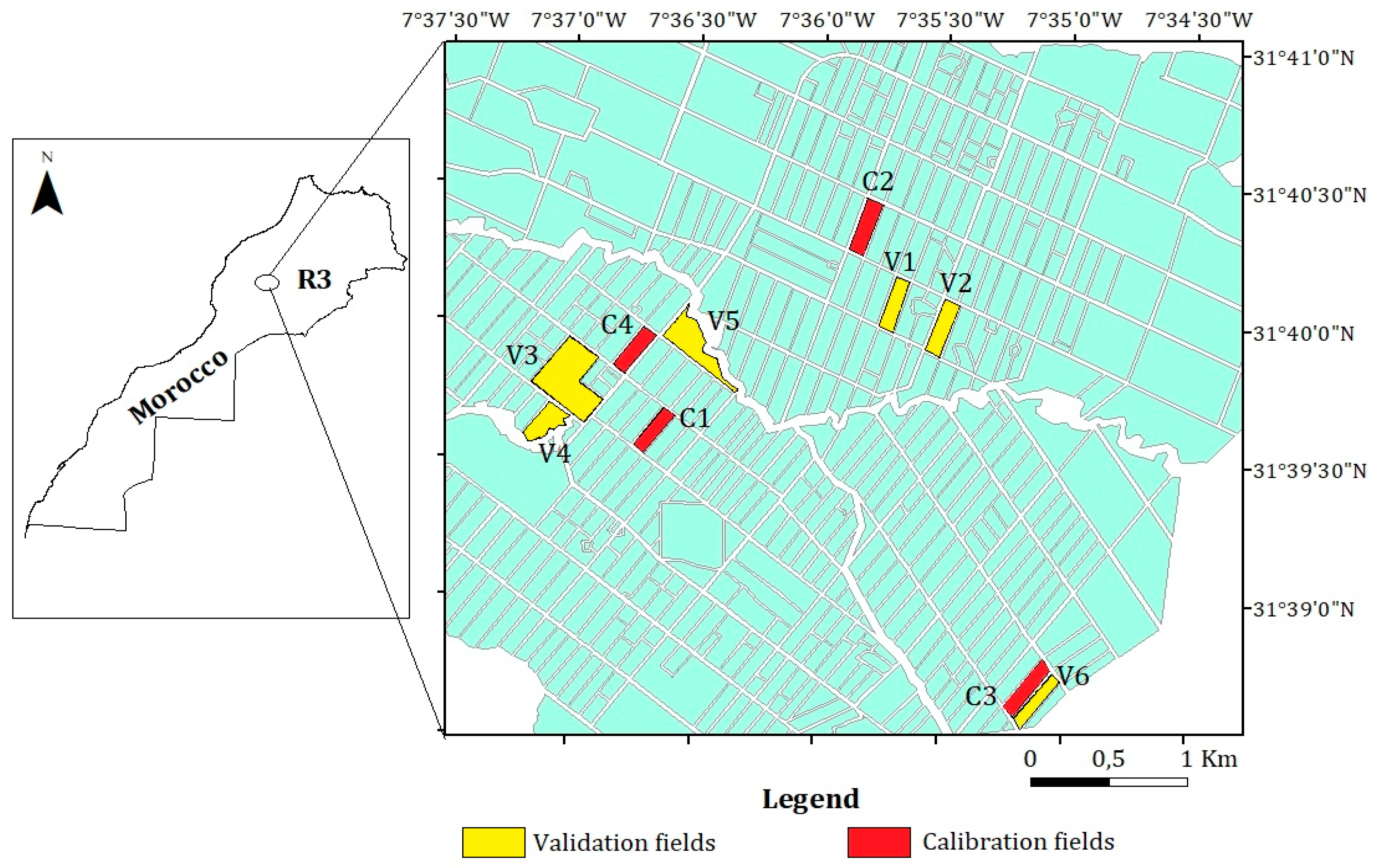
2.1.1. Study Area

The experiments were carried out in the R3 irrigated district located 40 km east of Marrakech city (Figure 1) during three growing seasons of winter wheat (2002–2003, 2008–2009, and 2012–2013). R3 is an irrigated area of about 2800 ha. The dominant crops are cereals, more wheat than barley [40]. Flood irrigation is widely practiced by the majority farmers in this area. The wheat is generally sown between mid-November and mid-January, depending on climatic conditions and the start of the rainfall season. The climate of this region is semi-arid, typically South-Mediterranean with high temperature in summer (38 °C, in July) and mild temperature in winter (5 °C, in February) with significant daily and monthly differences [41]. The average annual precipitation is about 250 mm, whereas the potential evapotranspiration (ET₀) is about 1600 mm/year [41].

The R3 district is practically flat. The total area is divided into different blocks, themselves separated into six rectangular plots with an area ranging from 3.5 to 5 ha. The irrigation in this area is managed jointly by three farmer associations in collaboration with the local center of the Regional Office of Agricultural Development of Haouz (ORMVAH). They play a key role on irrigation rounds management and on preparation of the irrigation scheduling according to sowing dates and the availability of water in the dam. At the beginning of agricultural season, a global amount of water is assigned to the irrigation sector. Managers and users decide the number of irrigations rounds and quantities assigned for the irrigation. At each round, the farmers receive an amount of water according to the owned area, without taking into account the type of crops and their water requirements. Additionally, ground water may be used for irrigation in limited cases, with priority for orchards, forages (alfalfa), and vegetables, but can also be used for cereal in case of high shortage of dam water. This complexity is compounded by the spatial heterogeneity of the sowing dates, the size of tilled plots, and the quantity of nitrogen used [42]. The result is a high spatial and temporal heterogeneity of irrigation water requirement that is not considered in water attribution.

2.1.2. Field Data

The meteorological data has been controlled by an automatic weather station installed near the study area. This station was equipped with instruments to measure global solar radiation (R_g), wind speed, precipitation, air temperature (T_a), and relative humidity.

For monitoring vegetation growth, measurements of dry matter (DM) and grain yield (GY) were performed on ten fields of wheat, during the 2002/2003, 2008/2009, and 2012/2013 growing seasons (

Table 1. Final dry matter (DM) and grain yield (GY) obtained for calibration (C1 to C4) and validation (V1 to V6) fields, conducted during 2002/2003, 2008/2009, and 2012/2013 wheat seasons.

Year	2002/2003				2008/2009				2012/2013
Field	C1	C2	V1	V2	C3	V3	V4	V5	C4	V6
DM (t/ha)	5.89	3.75	1.67	4.79	5.95	4.91	5.81	4.67	7.90	8.04
GY (t/ha)	2.87	1.98	0.9	2.51	2.81	2.44	2.96	2.44	4.15	4.42

). For more details about these experiments see Belaqziz et al. [30], Duchemin et al. [41], and Le Page et al. [43]. Along each season, vegetation samples were cut at ground level within squares of 0.5 × 0.5 m. On each sampling date, five samples were chosen randomly within each field for spatial representativeness issues. The fresh biomass was first weighed in the field by using a portable electric balance. Next, the various samples were placed in an oven at 85 °C for 72 h. Afterward, dry biomass was weighed again to determine the DM. The GY was also weighted at the start of the grain filling.

The fields named C_i (i = 1 to 4) were used for model calibration (Equations (12)–(15)). These fields were selected for their representativeness of the growth conditions for the three studied seasons (Table 1). However, the fields V_i (i = 1 to 6) were used for model validation (see, Section 2.2.3). Additionally, for additional validation of the model against AquaCrop model estimates, we used the data (climate, irrigation, and nutrient), relating to 112 wheat fields conducted in the study site (R3) during the 2008–2009 season, to run the two models [30].

2.1.3. Satellite Data

In this study, a set of surface reflectance images in the infrared (0.73–1.11 μm) and red (0.58–0.68 μm) bands have been used to determine the Normalized Difference Vegetation Index (NDVI) and the vegetation fraction cover, with high spatial resolution (10 to 30 m), for three agricultural seasons (

Table 2. Satellite images used to calculate wheat production during the 2002/2003, 2008/2009, and 2012/2013 agricultural seasons.

Year	Satellite Images	Images Number	Resolution (m2)
2002/2003	Landsat-TM7	5	30
	SPOT4	3	20
	SPOT5	2	10
2008/2009	Landsat-TM5	16	30
2012/2013	SPOT4	13	10
	Landsat8	5	30

). For those images, a radiometric calibration and atmospheric corrections were made based on the reflectance of invariant objects (bare soil, fallow, and houses) and were then transformed into NDVI maps.

-

For the 2002/2003 agricultural season, 10 images acquired by Landsat 7 Enhanced Thematic Mapper Plus (ETM+), SPOT4-HRVIR and SPOT5-HRG were exploited.

-

For the 2008–2009 agricultural season, 16 images from Landsat 5 Thematic Mapper (TM) sensor were collected [30]. Atmospheric correction was performed by the SMAC correction algorithm [44] using the aerosol optical depth measured at the Saada station near Marrakech city [45].

-

During the 2012/2013 agricultural season, 18 images obtained from the SPOT4and Landsat 8 Operational Land Imager (OLI) sensors were used. These images were acquired during 5 months between 31 January and 15 June 2013 [43]. Radiometric correction was performed by the Multi-Sensor Atmospheric Correction Software–Prototype [45,46].

For both SPOT and Landsat satellite images, the geometric correction was performed using the Ground Control Points collected during the experiment [40], followed by the radiometric correction which was achieved in three steps. Firstly, we corrected a “reference” image from atmospheric effects using the SMAC correction algorithm and standard values of atmospheric components. Secondly, the radiometry of each image was homogenized against this reference image thanks to a set of reliable invariant features. This normalization was performed by applying linear relationships, between the digital numbers of raw images and the reflectance values of the reference image [40]. Thirdly, an additional linear correction has been applied between the satellite NDVI values and the NDVI ground measurements collected using the hand-held Cropscan Multispectral Radiometer. This inter-calibration ensures a maximal agreement between satellite and in situ NDVI values.

2.2. Proposed Model

The proposed approach is based on the light-use-efficiency model developed by Monteith which uses the three efficiencies method as a basis [33,47]. This model exploits an energy approach relating the production of dry matter to the amount of solar radiation received by the plant, assuming that the accumulation of dry matter is proportional to the accumulation of photosynthetically active radiation (PAR) absorbed by the plant.

2.2.1. Dry Matter

The light-use-efficiency model is an agro-meteorological crop model, which is used to estimate the dry matter by introducing the radiation intercepted by the crop during a growing period. A semi-empirical equation based on three efficiencies is then used to calculate the daily production of dry matter as follows:

$$\mathsf{\Delta }\mathrm{DM}={\mathsf{\epsilon }}_{\mathrm{s}}\times {\mathsf{\epsilon }}_{\mathrm{i}}\times {\mathsf{\epsilon }}_{\mathrm{conv}}\times {\mathrm{R}}_{\mathrm{g}}\times \mathsf{\Delta }\mathrm{t}$$

(1)

with ΔDM (g m⁻²) is the dry matter produced during a period Δt. ${\mathsf{\epsilon }}_{\mathrm{s}},{\mathsf{\epsilon }}_{\mathrm{i}} \mathrm{and} {\mathsf{\epsilon }}_{\mathrm{conv}}$ represent the climatic efficiency, the light interception efficiency and the conversion efficiency of the radiation absorbed by the vegetation into biomass (g MJ⁻¹), respectively. R_g is the cumulative daily value of incident global radiation (MJ m⁻²) received by a horizontal plane above the vegetation.

-

Climatic efficiency, ${\mathsf{\epsilon }}_{\mathrm{s}}$

${\mathsf{\epsilon }}_{\mathrm{s}}$ is the ratio between PAR and R_g. PAR is the spectral band of solar radiation between 380 nm and 710 nm [48]. The value of ${\mathsf{\epsilon }}_{\mathrm{s}}$ varies between 0.42 (for direct radiation) and 0.65 (for diffuse radiation) with an average of 0.5 [49]. Additionally, Monteith [33] used the value of 0.5 as an average of ${\mathsf{\epsilon }}_{\mathrm{s}}$ for tropical and temperate regions. In the same range, Varlet-Grancher et al. [50], obtained an average value of ${\mathsf{\epsilon }}_{\mathrm{s}}$ equal to 0.48 for the Mediterranean climate. They also demonstrated that ${\mathsf{\epsilon }}_{\mathrm{s}}$ varies slightly depending on the solar elevation, cloud cover, and site latitude. In this study the value ${\mathsf{\epsilon }}_{\mathrm{s}}$ = 0.48 was used.

-

Interception efficiency, ${\mathsf{\epsilon }}_{\mathrm{i}}$

${\mathsf{\epsilon }}_{\mathrm{i}}$ is defined as the ratio between the PAR intercepted by the canopy (PARc) and the downward PAR (PAR_i). ${\mathsf{\epsilon }}_{\mathrm{i}}$ varies between 0 in the absence of green vegetation, and 0.95 for highly developed vegetation with full photosynthetic activity [51]. The calculation of this parameter depends essentially on the vegetation index, such as NDVI [52]. Often ${\mathsf{\epsilon }}_{\mathrm{i}}$ is linked to NDVI by a linear relationship [53]. In this study we used:

$${\mathsf{\epsilon }}_{\mathrm{i}}={\mathsf{\epsilon }}_{\mathrm{imax}} \frac{\mathrm{NDVI}-{\mathrm{NDVI}}_{\min }}{{\mathrm{NDVI}}_{\max }-{ \mathrm{NDVI}}_{\min }}={\mathsf{\epsilon }}_{\mathrm{imax}} \times \mathrm{NDVIn}$$

(2)

NDVI_min and NDVI_max are the minimum and maximum NDVI values observed during the wheat season in the study site. They correspond to the bare soil (NDVI_min = 0.14) and the totally covering vegetation for the entire time series of remote sensing data (NDVI_max = 0.92), respectively [41]. $\mathrm{NDVIn}= \frac{\mathrm{NDVI}-{\mathrm{NDVI}}_{\min }}{{\mathrm{NDVI}}_{\max }-{ \mathrm{NDVI}}_{\min }}$ is the normalized NDVI, and ${\mathsf{\epsilon }}_{\mathrm{imax}}$ is the maximum interception efficiency corresponding to the value of ${\mathsf{\epsilon }}_{\mathrm{i}}$ when NDVI=NDVI_max. ${\mathsf{\epsilon }}_{\mathrm{imax}}$ is then considered as a local characteristic of wheat growth. It depends on the canopy high, leaf area density, and the plant geometry at full development stage [54,55]. These canopy characteristics affect the scattering radiation within the canopy which is not measured by NDVI. Then, the coefficient ${\mathsf{\epsilon }}_{\mathrm{imax}}$ is considered as an empirical constant that must be determined under local conditions of wheat growth.

-

Conversion efficiency, ${\mathsf{\epsilon }}_{\mathrm{conv}}$

${\mathsf{\epsilon }}_{\mathrm{conv}}$ (g MJ⁻¹) characterizes the ability of a canopy to convert intercepted radiation into biomass. Indeed, ${\mathsf{\epsilon }}_{\mathrm{conv}}$ is defined as the ratio between the quantity of dry matter (DM) produced during a given period Δt and the PARc absorbed during the same period. This efficiency can be obtained experimentally, however there are great variations between studies [56]. Gosse et al. [57], recommended average ${\mathsf{\epsilon }}_{\mathrm{conv}}$ values of 1.93 g MJ⁻¹ and 2.51 g MJ⁻¹ for C3 and C4 crops, respectively. However, ${\mathsf{\epsilon }}_{\mathrm{conv}}$ can reach around 3.5 g MJ⁻¹ in optimal conditions. For wheat crops, the values of ${\mathsf{\epsilon }}_{\mathrm{conv}}$ are set between 1.80 and 2.40 g MJ⁻¹ [58], 1.47–1.74 g MJ⁻¹ [59], 1.2 g MJ⁻¹ [60], 2 g MJ⁻¹ [61], and 1.9 g MJ⁻¹ [62]. In addition, ${\mathsf{\epsilon }}_{\mathrm{conv}}$ declines under extreme agro-environmental conditions (water, nitrogen, temperature, and salinity stresses) [32,59].

The following equation is proposed to estimate ${\mathsf{\epsilon }}_{\mathrm{conv}}$:

$${\mathsf{\epsilon }}_{\mathrm{conv}}\left(\mathrm{t}\right)={\mathsf{\epsilon }}_{{\mathrm{conv}}_{\max }}\left(\mathrm{t}\right) \times { \mathrm{K}}_{{\mathrm{s}}_{\mathrm{conv}}}\times { \mathrm{K}}_{\mathrm{T}}$$

(3)

with ${\mathsf{\epsilon }}_{{\mathrm{conv}}_{\max }}\left(\mathrm{t}\right)$ is the maximum conversion efficiency (g MJ⁻¹), depending on the agro-environmental conditions, variety, and crop phenological stages [32,57,63,64,65]. ${\mathrm{K}}_{{\mathrm{s}}_{\mathrm{conv}}}$ is the water stress coefficient that affects vegetative production [42,66]. K_T is the temperature stress coefficient.

• Water stress coefficient ${\mathrm{K}}_{{\mathrm{s}}_{\mathrm{conv}}}$

To estimate ${\mathrm{K}}_{{\mathrm{s}}_{\mathrm{conv}}}$, a simple formulation based on the results of Toumi et al. [66], reinforced by Hadria et al. [42], and Jackson et al. [67], has been proposed. These studies demonstrated that the effect of water stress coefficient $K_s$ (defined by the FAO as the ratio between actual and maximal evapotranspirations) on yield production remains insignificant (less than 4%) when its value is situated between 0.7 and 1. Furthermore, keeping $K_s$ above 0.7 requires a significant increase in irrigation water [42,66]. In order to minimize the wasting of irrigation water so as not to affect the yield, we proposed the following formulation for ${\mathrm{K}}_{{\mathrm{s}}_{\mathrm{conv}}}$ estimating:

$$\{\begin{array}{c}{\mathrm{K}}_{{\mathrm{s}}_{\mathrm{conv}}}=1 \mathrm{for} K_s\ge 0.7\\ {\mathrm{K}}_{{\mathrm{s}}_{\mathrm{conv}}}=\frac{K_s}{0.7} \mathrm{for} K_s\le 0.7\end{array}$$

(4)

The water stress coefficient $K_s$ depends on the soil water availability. It is calculated from the water balance in the root zone following exactly the FAO-56 model detailed by Allen et al. [68]:

$$K_s=\frac{TAW-Dr}{TAW-RAW}=\frac{TAW-Dr}{\left(1-p\right)\times TAW}$$

(5)

Dr is the depletion of water in the root zone (mm) calculated by using daily rainfall (P) and irrigation (I). TAW is the total available water in the root zone (mm). RAW is the readily available water used by the plant (mm). Equation (5) is valid if Dr > RAW. When Dr < RAW, Ks is equal to 1. TAW and RAW are calculated as a function of the soil moistures at field capacity (${\theta }_{fc}$) and at wilting point (${\theta }_{wp}$).

$$TAW=1000 \times \left({\theta }_{fc}-{\theta }_{wp}\right) \times Z_r$$

(6)

$$RAW=p \times TAW$$

(7)

where $Z_r$ is the thickness of the root zone (mm) and p is a crop parameter which depends on the evapotranspiration under standard conditions ($E{T}_c$). For winter wheat and most cereals, the recommended value is p = 0.55 when $E{T}_c$ is around 5 mm/day (FAO-56, Table 2). When $E{T}_c$ differs to 5 mm/day, p can be adjusted using the following approximation:

$$p=0.55 + 0.04\times (5 - E{T}_c)$$

(8)

$E{T}_c$ is estimated from the NDVI by using the relationship developed by Duchemin et al. [41], for wheat crop grown in the studied site (R3).

• Temperature stress coefficient $K_T$

The thermal stress factor $K_T$ measures the restrictive effect of temperature on the conversion of intercepted solar radiation into plant biomass. Indeed, the low and high air temperatures, compared to the optimal temperature for growth and yield, decrease the rate of phytomass production [69]. The effect of temperature on the rate of production of phytomass is taken into account. For that reason, the daily average of air temperature (T_a) is integrated to an equation based on the optimal temperature ($T_{opt}$) (necessary for the plants growth) as well as on the two extreme values $T_{min}$ and $T_{max}$ (below and beyond which plant growth is assumed insignificant) as follows [69]:

$$\{\begin{array}{c}{K}_T=1-{\left(\frac{T_{opt}-T_a}{T_{opt}-T_{min}}\right)}^3 \mathrm{for} T_{min}<T_a<T_{opt } \\ K_T=1-{\left(\frac{T_{opt}-T_a}{T_{opt}-T_{max}}\right)}^3 \mathrm{for} T_{opt}<T_a<T_{max} \\ K_T=0 for T_a<T_{min} \mathrm{and} T_a>T_{max} \end{array}$$

(9)

The values of $T_{min}, T_{opt} \mathrm{and} T_{max}$ used in this study were 5, 26, and 33 °C, respectively [42,66].

Following the above development, the Equation (1) of dry matter becomes:

$$\mathsf{\Delta }\mathrm{DM}=0.48 \times ({\mathsf{\epsilon }}_{\mathrm{imax}} \times {\mathsf{\epsilon }}_{{\mathrm{conv}}_{\max }}\left(\mathrm{t}\right)) \times { \mathrm{K}}_{{\mathrm{s}}_{\mathrm{conv}}} \times { \mathrm{K}}_{\mathrm{T}} \times { \mathrm{NDVI}}_{\mathrm{n}} \times { \mathrm{R}}_{\mathrm{g}} \times \mathsf{\Delta }\mathrm{t}$$

(10)

Finally, in order to reduce the number of unknown parameters, we replaced the product $({\mathsf{\epsilon }}_{\mathrm{imax}}.{\mathsf{\epsilon }}_{{\mathrm{conv}}_{\max }}\left(\mathrm{t}\right))$ by a single parameter ${\mathsf{\epsilon }}_{\max }\left(\mathrm{t}\right)$. Then, Equation (10) is rewritten as:

$$\mathsf{\Delta }\mathrm{DM}=0.48 \times { \mathsf{\epsilon }}_{\max }\left(\mathrm{t}\right) \times { \mathrm{K}}_{{\mathrm{s}}_{\mathrm{conv}}}\times { \mathrm{K}}_{\mathrm{t}} \times { \mathrm{NDVI}}_{\mathrm{n}} \times {\mathrm{R}}_{\mathrm{g}} \times \mathsf{\Delta }\mathrm{t}$$

(11)

In conclusion, ∆DM is expressed by using a single parameter $({\mathsf{\epsilon }}_{\max })$, three indices $\left({\mathrm{K}}_{{\mathrm{s}}_{\mathrm{conv}}},{ \mathrm{K}}_{\mathrm{T}} \mathrm{and} \mathrm{NDVI}\right)$ and one meteorological variable (R_g). ${\mathsf{\epsilon }}_{{\mathrm{conv}}_{\max }}\left(\mathrm{t}\right)$ can then integrate the effects of nitrogen stress, the carbon assimilation rate of the leaves (which depends on the phenological stages) and the possible interactions between these two factors and water and temperatures stresses.

From the appearance of the ears, the simple calculation of the dry matter dynamic remains insufficient to monitor the grain filling. The latter is controlled by the process of partitioning the produced DM between grains and straw. The Harvest Index (HI) evaluates this partitioning [70].

2.2.2. Harvest Index, HI

HI is the ratio between the grain’s weight and the total dry matter produced at the time t. In this study, the dynamic of HI is modeled in two periods:

-

Linear increase of HI which begins at flowering (time t_start, after sowing date) and ends when HI reaches its final value HI₀ (time t_end). This type of correlation has been used by other studies [71,72,73]. Thus, HI is modeled by the following equation:

$$\mathrm{HI}=\frac{{\mathrm{HI}}_0}{\left({\mathrm{t}}_{\mathrm{end}}-{\mathrm{t}}_{\mathrm{start}}\right)} \times \left(\mathrm{t}-{\mathrm{t}}_{\mathrm{start}}\right)$$

(12)

-

Constant value of HI (HI = HI₀).

${\mathrm{t}}_{\mathrm{start}}$ and ${\mathrm{t}}_{\mathrm{end}}$ and HI₀ are local parameters, which will be derived from the field measurements.

The advantage of this approach lies in its simplicity which intrinsically combines: (i) The storage of a part of DM assimilation in the ear, and (ii) avoid the requirement of the number and weight of the grain/ear to predict the grain yield [23,74,75,76]. In fact, HI integrates the effect of water stress over different periods of the crop development phases. This has been confirmed for different types of crops by several studies carried out on cereals in Africa [77,78,79], in North America [80], in Europe [81], and globally [82].

For the determination of the final harvest index ${\mathrm{HI}}_0$, we were inspired by the work carried out by Jianqiang et al. [28], Becker-Reshef et al. [29], and Belaqziz et al. [30], who implemented operational methods for forecasting grain yields based on NDVI data. ${\mathrm{HI}}_0$ is calculated as follows:

$${\mathrm{HI}}_0={\mathrm{HI}}_{0\max }-\mathsf{\Delta }{\mathrm{HI}}_0 \times \left(\frac{{\mathrm{NDVI}}_{{\max }_{\max }}-{\mathrm{NDVI}}_{\max }}{{\mathrm{NDVI}}_{{\max }_{\max }}-{\mathrm{NDVI}}_{{\max }_{\min }}}\right)$$

(13)

where ${\mathrm{HI}}_{0\max }$ is the maximum value of ${\mathrm{HI}}_0$ observed in the study area and $\mathsf{\Delta }{\mathrm{HI}}_0$ its variation range. ${\mathrm{NDVI}}_{{\max }_{\max }}{ \mathrm{and} \mathrm{NDVI}}_{{\max }_{\min }}$ are the maximum and the minimum values of the ${\mathrm{NDVI}}_{\max }$ over the study area, respectively. Then following this formulation (Equation (13)), HI₀ varies from $({\mathrm{HI}}_{0\max }-\mathsf{\Delta }{\mathrm{HI}}_0)$ to ${\mathrm{HI}}_{0\max }$, depending on the values of NDVI_max.

Finally, the grain yield GY, at the time t, is deduced by:

$$\mathrm{GY}\left(\mathrm{t}\right)=\mathrm{DM}\left(\mathrm{t}\right) \times \mathrm{HI}\left(\mathrm{t}\right)$$

(14)

where DM(t) is the sum of ∆DM values from plant emergence until the time t.

As a summary, the

Table 3. List of the parameters of the proposed model.

	Notation	Description	Unit	Value
Inputs	NDVI	Normalized Difference Vegetation Index	-	-
	Rg	Incoming solar radiation	MJ/m2	-
	Ta	Daily average air temperature	°C	-
	P	Rainfall	mm	-
	I	Irrigation	mm	-
Constants	Tmin, Topt, Tmax	Temperature for growth	°C	5, 26, 33
	NDVImax	Maximum value of NDVI	-	0.92
	NDVImin	Minimum value of NDVI	-	0.14
	εi	Climatic efficiency	-	0.48
	θfc	Soil moisture at field capacity	m3/m3	0.32
	θwp	Soil moisture at wilting point	m3/m3	0.17
	HI0	Final harvest index	-	0.50 *
	HI0max	Maximum value of HI0	-	0.59 *
	∆HI0	Variation range of HI0	-	0.15 *
Outputs	DM	Aboveground dry matter	t/ha	-
	GY	Grain yield	t/ha	-

* Calibrated, see Section 3.2.

groups together the various parameters of the presented simple model.

2.2.3. Model Calibration and Validation

The model calibration was performed in two stages:

-

Inverting the Equation (11) to determine the local values of the parameter ${\mathsf{\epsilon }}_{\max }$ as follows:

$${\mathsf{\epsilon }}_{\max }\left(\mathrm{t}\right)=\frac{\mathsf{\Delta }\mathrm{DM}}{0.48 \times { \mathrm{K}}_{{\mathrm{s}}_{\mathrm{conv}}} \times { \mathrm{K}}_{\mathrm{T}} \times { \mathrm{NDVI}}_{\mathrm{n}} \times { \mathrm{R}}_{\mathrm{g}} \times \mathsf{\Delta }\mathrm{t}}$$

(15)

Initially the values of ${\mathsf{\epsilon }}_{\max }$ will be calculated by Equation (15) fed by the observed data of the evolution of DM, R_g, and NDVI for the fields named C_i (i = 1 to 4, Table 1). In the second step, ${\mathsf{\epsilon }}_{\max }$ is correlated to the cumulative growing degree days (CGDD) calculated from the sowing date. The CGDD values were daily calculated by subtracting the wheat base temperature (T_min) from the daily average of air temperature (T_a) [76]:

$$\mathrm{CGDD}={{\displaystyle \sum }}^{ }\left({\mathrm{T}}_{\mathrm{a}}-{\mathrm{T}}_{\min }\right)$$

(16)

For analyzing the obtained relationship ${\mathsf{\epsilon }}_{\max }\left(\mathrm{CGDD}\right)$, the Brower phenological scale is used. This scale, described in detail by Laguette et al. [56], presents a finer agronomic description of the cereal development cycle. It allows classifying visible phenological stages in 21 steps easy to interpret: from 1 to 5 for the vegetative phase, from 6 to 17 for reproduction period, and from 18 to 21 for grain ripening.

-

Adjustment of Equation (12), by using data for the fields C_i (i = 1 to 4), to determine the local values of ${\mathrm{t}}_{\mathrm{start}}$, ${\mathrm{t}}_{\mathrm{end}}$, and HI₀.

After, the calibrated model is validated by using the observed data collected for six fields V_i (i = 1 to 6, Table 1), especially the temporal evolution of biomass and grain weight. In addition, further validation has been done through the comparison with the final biomass and grain yield calculated by AquaCrop model [17,83], previously calibrated for the study area [66]. For that purpose, the concerned fields are V_i (i = 1 to 6) and the 112 fields mentioned in Section 2.1.2.

2.2.4. Model Evaluation Metrics

The estimated DM and GY by the proposed model were compared to the observed values and those estimated by AquaCrop model using the determination coefficient (R²) of the regression line and the Root Mean Square Error (RMSE):

$${\mathrm{R}}^2=\frac{{\left({{\displaystyle \sum }}_{\mathrm{i}=1}^{\mathrm{n}}\left({\mathrm{Y}}_{\mathrm{i}}- \overline{\mathrm{Y}}\right) \left({\mathrm{X}}_{\mathrm{i}}- \overline{\mathrm{X}}\right)\right)}^2}{\left[{{\displaystyle \sum }}_{\mathrm{i}=1}^{\mathrm{n}}{\left({\mathrm{Y}}_{\mathrm{i}}- \overline{\mathrm{Y}}\right)}^2\right]\left[{{\displaystyle \sum }}_{\mathrm{i}=1}^{\mathrm{n}}{\left({\mathrm{X}}_{\mathrm{i}}- \overline{\mathrm{X}}\right)}^2\right]}$$

(17)

$$\mathrm{RMSE}=\sqrt{\frac{1}{\mathrm{n}} {\displaystyle \sum }_{\mathrm{i}=1}^{\mathrm{n}}{\left({\mathrm{Y}}_{\mathrm{i}}-{\mathrm{X}}_{\mathrm{i}}\right)}^2}$$

(18)

where Y_i is the predicted value by the proposed model, X_i is the observed value or that estimated by AquaCrop model, $\overline{\mathrm{Y}}$ is the mean of Y_i values, $\overline{\mathrm{X}}$ is the mean of X_i values, and n is the number of observation.

Additionally, the performance of proposed model was compared to AquaCrop model by using the statistics of linear models presented in Coursol (1983) [84], which evaluate the statistical significance of the similarity between two regression lines (see Appendix A).

3. Results and Discussion

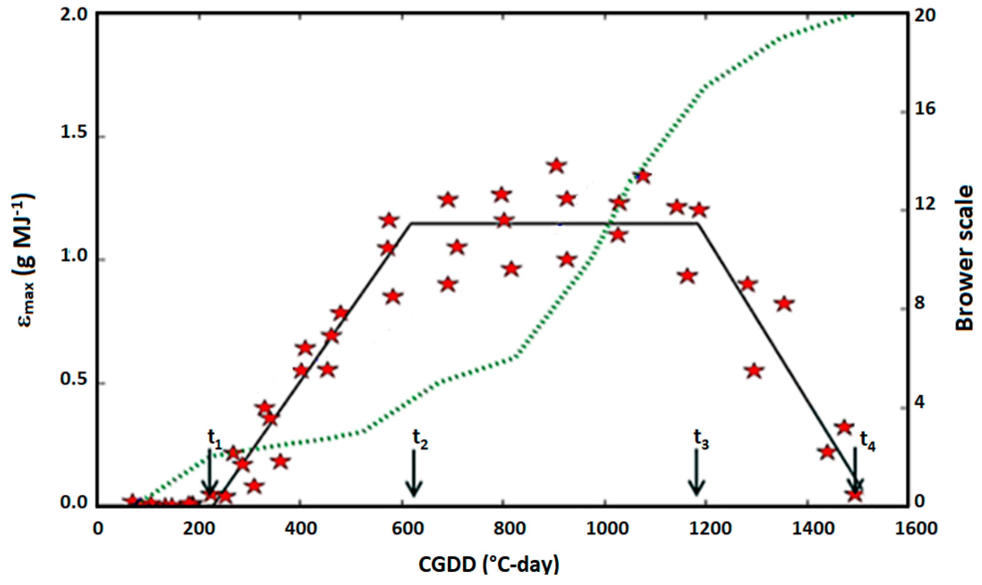
3.1. Calibration of ${\epsilon }_{max}$

As mentioned above, the calibration of ${\mathsf{\epsilon }}_{\max }$ consists of modeling its temporal dynamic as a function of CGDD. This evolution of ${\mathsf{\epsilon }}_{\max }$ is attributed to the seasonal change of conversion efficiency [32,63]. Indeed, Equation (15) is used to calculate the decadal values of ${\mathsf{\epsilon }}_{\max }$ by using data (R_g, T_a, NDVI, DM) observed over four fields of wheat (C1–C4, Table 1). The obtained results, presented in Figure 2, show that four stages can be distinguished in the evolution of ${\mathsf{\epsilon }}_{\max }\left(\mathrm{CGDD}\right)$:

Stage 1: ${\mathsf{\epsilon }}_{\max }$ is practically zero, from emergence to thermal time t₁,

Stage 2: Rapid increase in ${\mathsf{\epsilon }}_{\max }$ to its maximum value 1.15 g MJ⁻¹. This stage occurs between times t₁ and t₂,

Stage 3: ${\mathsf{\epsilon }}_{\max }$ remains practically constant at its maximum value 1.15 g MJ⁻¹ (the average value between t₂ and t₃),

Stage 4: Almost linear decrease of ${\mathsf{\epsilon }}_{\max }$, from its maximum value (in t₃) to a low value (in t₄).

As mentioned above, to determine the meaning of articulation times (t₁–t₄), we used the Brower scale of wheat development. Thus:

▪

t₁ = 230 °C-day: This time corresponds to the stage 2 of the Brower scale. This shows that t₁ coincides perfectly with the start of tillering. This result is reinforced by Hadria et al. [42], who obtained tillering at a CGDD equivalent to 260 °C-day. This work was calibrated and validated by the STICS model on wheat crops over our study area R3.

▪

t₂ = 620 °C-day: Is the thermal time corresponding to the start of the plateau phase. This time coincides with the stage 4 of the Brower scale wich corresponds to the end of tillering and the start of upstream stages. This time is characterized by the transition from leaf production to that of spikelets [85]. The obtained t₂ value is slightly lower than the CGDD = 696 °C-day estimated by Toumi et al. [66], for the start of the maximum of cover fraction.

▪

t₃ = 1186 ° C-day: Is the time of the end of the plateau phase which corresponds to the time between stages 16 and 17 of the Brower scale. It coincides with the end of flowering and the beginning of maturity of the wheat crop.

▪

t₄ = 1500 °C-day: Corresponds to the end of maturity of the wheat. This time coincides well with the CGDD at wheat maturity (1462 °C-day) obtained by Toumi et al. [66].

According to this description, we note that phase 1 (from emergence to t₁) is characterized by very low values of ${\mathsf{\epsilon }}_{\max }$. Thus, for this period ${\mathsf{\epsilon }}_{\max }$ is assumed to be zero. Additionally, for phase 3 we have assigned to ${\mathsf{\epsilon }}_{\max }$ the average of the values calculated between t₂ and t₃. However, for the two phases 2 and 4, the equations of ${\mathsf{\epsilon }}_{\max }$ were derived based on the linear regression. The corresponding coefficients of determination (R²) are 0.96 (n = 15) and 0.91 (n = 7) for phases 2 and 4, respectively. Thus, according to the results of this calibration, ${\mathsf{\epsilon }}_{\max }$ is parameterized as follow:

$${\mathsf{\epsilon }}_{\max }= \{\begin{array}{c}0\\ 0.003 \times \mathrm{CGDD}-0.68\\ 1.15\\ -0.0028 \times \mathrm{CGDD}+4.3\end{array}\begin{array}{c} \mathrm{for}\\ \mathrm{for}\\ \mathrm{for}\\ \mathrm{for}\end{array}\begin{array}{c}\mathrm{CGDD}\le 230 { }^{°}\mathrm{C}\\ 230 { }^{°}\mathrm{C}-\mathrm{day}<\mathrm{CGDD}\le 620 { }^{°}\mathrm{C}-\mathrm{day}\\ 620 { }^{°}\mathrm{C}-\mathrm{day}<\mathrm{CGDD}\le 1186 { }^{°}\mathrm{C}-\mathrm{day}\\ 1186 { }^{°}\mathrm{C}-\mathrm{day} <\mathrm{CGDD}\le 1500 { }^{°}\mathrm{C}-\mathrm{day}\end{array}$$

(19)

This expression reflects clearly the impact of the phenological stages on the coefficient ${\mathsf{\epsilon }}_{\max }$. In this context, Arkebauer et al. [32], and Asrar et al. [63] have shown that the values of ${\mathsf{\epsilon }}_{\mathrm{conv}}$ vary significantly with the wheat phenological stages. Generally, the values of ${\mathsf{\epsilon }}_{\mathrm{i}}$ and ${\mathsf{\epsilon }}_{\mathrm{conv}}$ are low during the initial phase [63]. However, during the growing stage (between t₁ and t₂) the increase in ${\mathsf{\epsilon }}_{\max }$ may be explained by the gradual increase of the carbon assimilation rate of the leaves required for the canopy expansion and for DM storage within the leaves fully emerged [17,18]. During the plateau phase (from t₂ to t₃), there is no canopy expansion, but the conversion coefficient remains maximum, because of grain filling which requires a high photosynthetic activity [17,18]. During the last phase (from t₃ to t₄), which coincides with the grain maturity stage and progressive senescence of the vegetation, the carbon assimilation rate of the leaves decreases [17,63]. This can explain the linear decrease in ε_max.

Moreover, the conversion coefficient ${\mathsf{\epsilon }}_{\mathrm{conv}}$ is also affected by vegetation water status. In this context, Muchow and Davis [86], have shown that ${\mathsf{\epsilon }}_{\mathrm{conv}}$ is more affected by crop water stress than ${\mathsf{\epsilon }}_{\mathrm{i}}$. Additionally, for cereals, Muchow [87], showed that the plant water status may impact the interception coefficient (${\mathsf{\epsilon }}_{\mathrm{i}})$ during the first six weeks. After this period, ${\mathsf{\epsilon }}_{\mathrm{conv}}$ is the most affected. In the same context, Asrar et al. [63] showed that just after irrigation, in the middle of the wheat season, ${\mathsf{\epsilon }}_{\mathrm{conv}}$ increased from 3 to 3.22 g MJ⁻¹.

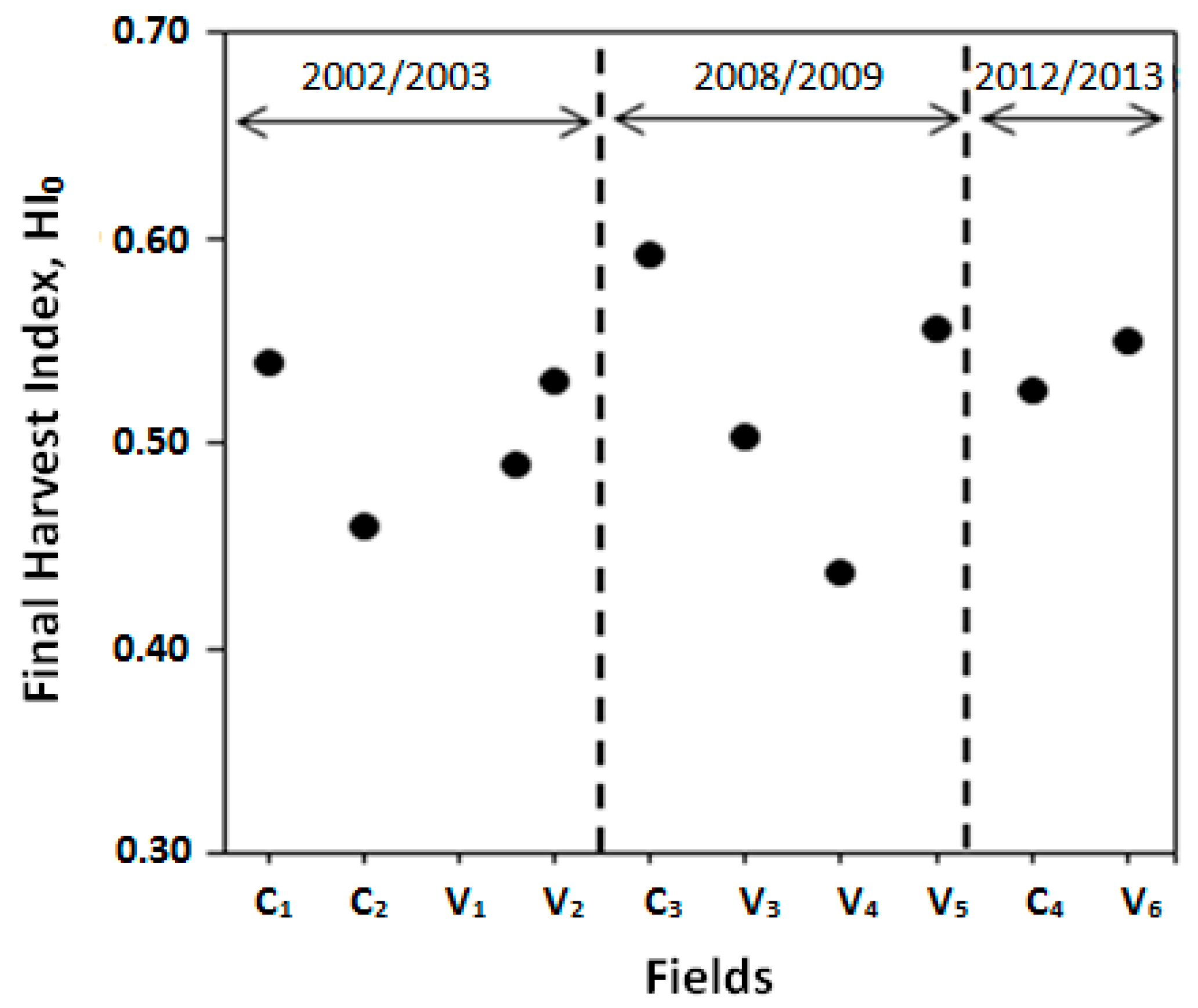
3.2. Calibration of HI

Figure 3 shows the evolution of HI as a function of CGDD obtained for the calibration fields C_i (i = 1 to 4, Table 1). This trend is segmented into two parts. The first one is characterized by a linear increase between t_start and t_end which fits well with the grains filling and maturity stages. The linear adjustment of Equation (12) led to the values of t_start = 750 °C-day and t_end = 1313 °C-day. For the second part (after t_end), HI keeps constant at its final HI₀, reached at the end of the wheat growing season. Following the data used in this calibration HI₀ = 0.50. This value is comparable to those obtained by other studies on wheat, such as Toumi et al. [66] in Morocco (HI₀ = 0.46), Moriondo et al. [88] in South America (HI₀ = 0.48), Jin et al. [89] in the northern plain of China (HI₀ = 0.46) and Hammer and Muchow [90] in northern Europe (HI₀ = 0.55).

Consequently, for the study region, the Equation (12) becomes:

$$\mathrm{HI}\left(\mathrm{CGDD}\right)=\frac{{\mathrm{HI}}_0}{563} \times \left(\mathrm{CGDD}-750\right)$$

(20)

The value 563 °C-day is the difference between t_end and t_start.

Furthermore, HI₀ can exhibit significant annual variability [28,29], which essentially results in the combination of the agro-environmental and climatic effects [6]. Hence the interest of the equation 13, which calculates HI₀ according to its maximum value observed in the study region (HI_0max) and its variation interval ΔHI₀. The determination of these two characteristics (HI_0max and ΔHI₀) is made by using data from 10 fields monitored during 3 wheat seasons 2002/2003, 2008/2009, and 2012/2013 (Table 1, Figure 4). It can be seen, that the HI_0max value observed in the study region is about 0.59 and the interval ΔHI₀ is 0.15. The obtained value of HI_0max is in the range (0.51–0.64) reported by Balaghi et al. [6], observed in other Moroccan regions. This study shows that HI_0max depends on the climate, the sowing date, and the rainfall/irrigation of the agricultural season. These conditions affect the value of the field’s NDVI_max. In our case, depending on the NDVI_max value, HI₀ of the field can vary from 0.44 (=0.59–0.15) to 0.59.

Finally, for this proposed model, the two relationships ε_max (CGDD) and HI(CGDD) (equations 19 and 20, respectively) represent the local agro-environmental characteristics of wheat production. They implicitly integrate the effects of different factors affecting crop development and yield which were not considered explicitly in the Equation (11), especially nutrient stress, soil quality, wheat variety, etc. Thus, these two parameters represent the calibration keys of the proposed method for other sites having other agro-environmental characteristics.

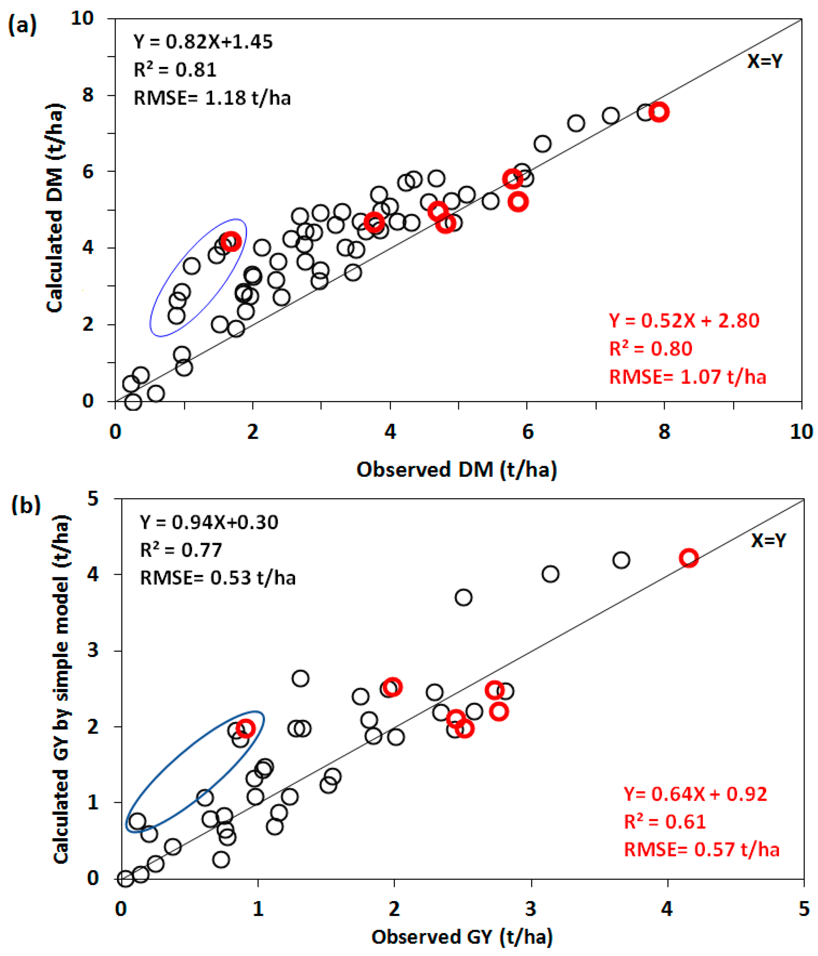
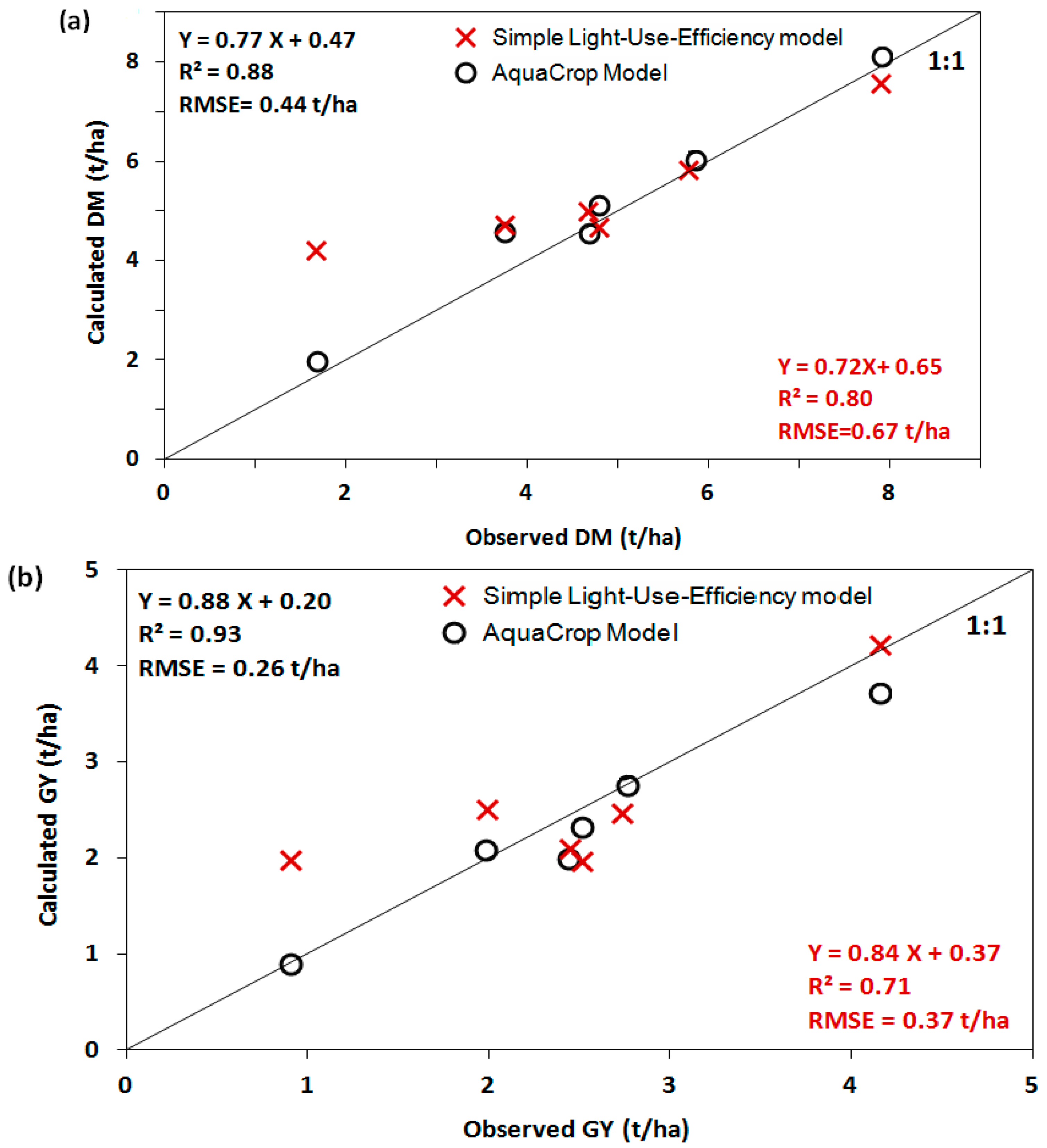
3.3. Model Validation by Using the Observed Data

Figure 5 displays the comparison between the simulated and the observed dry matter (DM) and grain yield (GY) during the wheat development, for the six validation fields (V_i), conducted during the 2002/2003, 2008/2009, and 2012/2013 wheat growing seasons. From this figure, it can be seen that there is a good agreement between the simulated and observed yields (DM and GY). Indeed, for DM (Figure 5a, black circles), the values of R² and the slope of the linear regression line are 0.81 and 0.82, respectively. Additionally, the RMSE value is around 1.18 t/ha, which represents about 17% of the average value of DM observed. For the evolution of the grain filling (Figure 5b, black circles), the statistical values of the comparison between simulation and observation results are also satisfying. The values of R², the slope, and the RMSE are 0.77, 0.94, and 0.53 t/ha, respectively.

Regarding the final DM and GY yields (Figure 5, red circles), the performance of the proposed approach is very promising. The RMSE values are 1.07 and 0.54 t/ha for DM and GY, respectively. These values are acceptable by comparison to the observed average final yields: 5.65 t/ha for DM and 2.70 t/ha for GY. The accuracy of the simple proposed approach is practically similar to the one obtained by more complex models of crops development and yield. Indeed, for the study area (R3), the STICS model [75] reproduced the final biomass and grain yields with RMSE equal to 1.35 and 0.87 t/ha [42]. Additionally, using the AquaCrop model, Mkhabela and Bullock [91] estimated the wheat grain yield for five sites in Western Canada from 2003 to 2006, with an error of about 24%. Similarly, the WOFOST model estimated the final yield, for six European regions, with an average error of 13 and 19% for the DM and the GY, respectively [56].

Furthermore, for the field V1 invaded by oats during the 2002–2003 season [41], the observed DM and GY (indicated by the blue oval marking in Figure 5) are clearly overestimated by the proposed approach, which simulates the absorbed solar radiation using remotely sensed NDVI. The same result was underlined by Hadria et al. [42], and Toumi et al. [66], who monitored the wheat yield in the same study area (R3) by using STICS and AquaCrop models, respectively. Otherwise, for the DM between 1.5 and 5 t/ha, corresponding mainly to the stages before maturity, the model overestimates the observations with an almost systematic difference of about 1 t/ha (Figure 5a). Fortunately, this overestimation of DM did not affect the estimations of grain yield (Figure 5b).

Overall, the yield predictions (DM and GY) by the proposed approach are very encouraging for the six validation fields. The observed differences between observed and simulated production can be explained by the difference between the calibration and validation fields in terms of soil texture [92] and the nutrient applied. Currently, the proposed model does not take explicitly into account the nutrient stress. The latter is considered implicitly through the calibrated agro-environmental characteristics ε_max (Equation (19)) and HI (Equation (20)) overall for the studied area.

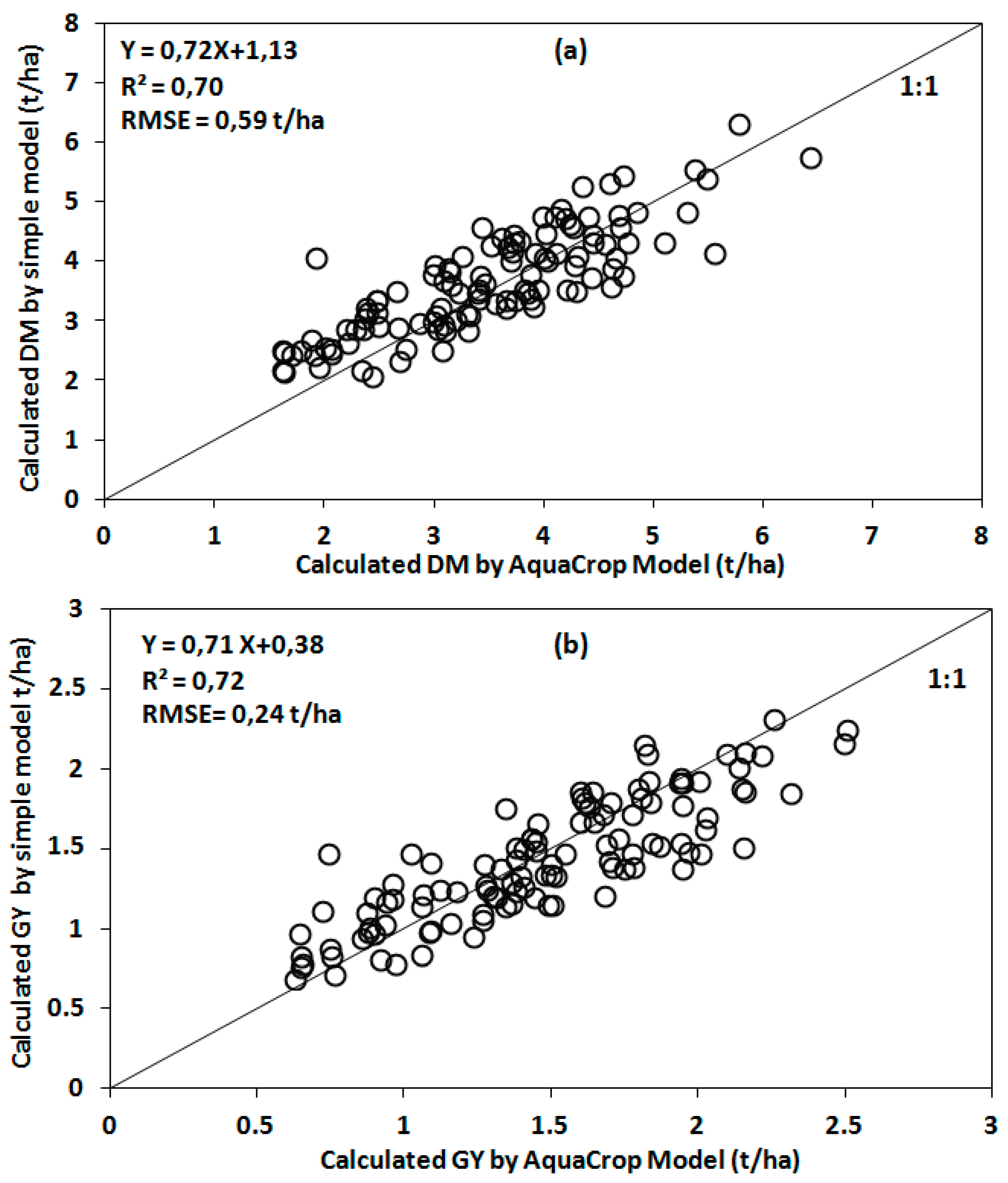
3.4. Model Evalution against AquaCrop Model

In order to go further in the evaluation of the proposed approach, the estimated DM and GY by this approach were also compared with the AquaCrop model simulations on six fields V_i (Table 1) monitored during three wheat seasons (Figure 6). These results showed that, despite its simplicity, the statistical performance of the proposed approach is close to that of the AquaCrop model, which is much more complex and very greedy in input parameters [76]. Indeed, for the DM estimations, the slope, the intercept of the regression line, the determination coefficient (R²) and the RMSE are respectively 0.72, 0.65 t/ha, 0.8 and 0.67 t/ha for the proposed model and 0.77, 0.47 t/ha, 0.88 and 0.44 t/ha for AquaCrop. Additionally, for GY estimations, the values of these statistical metrics are respectively 0.84, 0.37 t/ha, 0.71 and 0.37 t/ha for the developed model and 0.88, 0.20 t/ha, 0.93 and 0.26 t/ha for AquaCrop. According to the statistics of linear models (Appendix A), it is easily deduced that the two regression lines of AquaCrop and the proposed model are not significantly different p < 0.01) for both DM and GY.

Additionally, Figure 7 presents the comparison between the final dry matter (DM) and grain yield (GY) simulated by the AquaCrop and the proposed models for 112 fields conducted during the 2008/2009 wheat season. The statistical parameters of this comparison are also encouraging; the slope, the intercept, R² and RMSE are respectively 0.72, 1.13 t/ha, 0.70 and 0.59 t/ha for DM and 0.71, 0.38 t/ha, 0.72 and 0.24 t/ha for GY. For both models, the slope and R² values are close to 1 and the intercepts and RMSEs are statistically small compared to the average values obtained for DM and GY.

The differences obtained between the two model estimates may be due to their schemes used to represent the effect of water stress on the growth, development, and yield [93,94]. Indeed, the AquaCrop model describes finely the effects of the plant water status on DM development by using a dynamic function of water stress taking into account the expansion of the leaves, the stomata closing and the senescence for the crop [17,76]. Thus, in AquaCrop, under limited water conditions, the plant transpiration is directly affected. On the other hand, the developed model used a simple relation (Equation (3)) to monitor the water stress effects on the conversion coefficient ε_conv. This effect has been alleviated by the proposal of a new formulation of the stress coefficient (K_{s_conv}, Equation (4)) to optimize the irrigation water supply [42,66]. This may explain the overestimation obtained in some fields, by the proposed approach, of the yields calculated by AquaCrop, especially for DM lower than 3 t/ha (Figure 7a) and GY lower than 1.5 t/ha (Figure 7b).

Additionally, for AquaCrop, carbon sequestration and nitrogen absorption are mainly linked to radiation and nitrogen limitations [17,76]. However, for the proposed model, the effect of nitrogen is incorporated into local ε_max calibration (Equation (19)). This correlation represents the integrating effect of the regional agro-environmental conditions (e.g., soil fertility and salinity) on crop yield.

4. Conclusions

The main objective of this work was to present a simple and enhanced light-use-efficiency model for monitoring the wheat crop yield in the semi-arid area. The model links the biomass production to the solar radiation received by the plant, assuming that the increase of the biomass produced is proportional to the accumulation of photosynthetically active radiation absorbed. The originality of the method consists in: (1) The expression of the conversion coefficient (${\mathsf{\epsilon }}_{\mathrm{conv}}$) by considering an appropriate stress threshold (k_sconv) for triggering irrigation, (2) the substitution of the product of the two maximum coefficients of interception (ε_imax) and conversion (ε_{conv_max}) by a single parameter ε_max, (3) the modeling of ${\mathsf{\epsilon }}_{\max }$ as a function of the Cumulative Growing Degree Days (CGDD) since sowing date, and (4) the dynamic expression of the harvest index (HI) as a function of the CGDD and the final harvest index HI₀ depending on the maximum values of Normalized Difference Vegetation Index (NDVI) in the studied area.

The model calibration reflects the impact of the phenological stages and water stress on the ${\mathsf{\epsilon }}_{\max }$ coefficient. Thus, the expression of ${\mathsf{\epsilon }}_{\max }$ as a function of CGDD has been segmented into four parts. However, a linear evolution was sufficient to represent the evolution of HI according to the CGDD up to its final value (HI₀ = 0.50) obtained in 1313 °C-day. Thus, the ${\mathsf{\epsilon }}_{\max }$ and HI equations are considered representative of the agro-environmental conditions of the Haouz plain. Therefore, they are considered the calibrating keys of the proposed approach in other different agro-environmental situations.

The model validation was performed against dry matter (DM) and grain yield (GY) observed during three wheat growing seasons and calculated by AquaCrop (more complex model). The obtained results reflect a satisfactory ability of the proposed approach to reproduce DM and GY. The values of R² and RMSE are of about 0.81 and 1.18 t/ha and 0.77 and 0.53 t/ha for monitoring the observed dynamics of DM and GY, respectively. For the final yield, the R² and RMSE are 0.8 and 1.07 t/ha and 0.81 and 0.57 t/ha for DM and GY, respectively. Against Aquacrop, the performance of the proposed model is very encouraging. Indeed, for DM, the R² and RMSE values are respectively 0.8 and 0.67 t/ha for the proposed model and 0.84 and 0.44 t/ha for AquaCrop. For the GY estimate, the values of these statistical metrics are respectively 0.71 and 0.37 t/ha for the developed approach and 0.93 and 0.26 t/ha for AquaCrop.

The integration of satellite data to the proposed model seems to be one of the most appropriate quantitative analysis methodologies that may be adopted for yield estimation at large spatial scales [95]. Indeed, the recent advent of new satellite sensors with both high spatial (less than 10 m), temporal resolution (less than 1 week), and multi-bands (optic, thermal, and microwave) as well as the developed computer processing tools have opened up new perspectives for mapping crop type [95] and field-level crop productivity [96]. This will allow the daily monitoring of the stress coefficient and the determination of the irrigations carried out necessary for the establishment of yield maps at large scales.

References

1. Le Page, M.; Zribi, M. Analysis and predictability of drought in Northwest Africa using optical and microwave satellite remote sensing products. Sci. Rep. 2019, 9, 1466. [Google Scholar] [CrossRef] [PubMed] [Green Version]
2. Dettori, M.; Cesaraccio, C.; Duce, P. Simulation of climate change impacts on production and phenology of durum wheat in Mediterranean environments using CERES-Wheat model. Field Crops Res. 2017, 206, 43–53. [Google Scholar] [CrossRef]
3. Bolle, H.J. Mediterranean Climate: Variability and Trends; Springer: Berlin/Heidelberg, Germany, 2002; ISBN 978-3540438380. [Google Scholar]
4. Bleu, P. Etat de L’environnement et du Développement en Méditerranée; Centre D’activités Régionales PNUD/PAM: Athens, Greece, 2009; p. 208. [Google Scholar]
5. Matesanz, S.; Valladares, F. Ecological and Evolutionary Responses of Mediterranean Plants to Global Change. Environ. Exp. Bot. 2014, 103, 53–67. [Google Scholar] [CrossRef] [Green Version]
6. Balaghi, R.; Tychon, B.; Eerens, H.; Jlibene, M. Empirical regression models using NDVI, rainfall and temperature data for the early prediction of wheat grain yields in Morocco. Int. J. Appl. Earth Obs. Geoinf. 2008, 10, 438–452. [Google Scholar] [CrossRef] [Green Version]
7. Kharrou, M.H.; Er-Raki, S.; Chehbouni, A.; Duchemin, B.; Simonneaux, V.; Le Page, M.; Ouzine, L.; Jarlan, L. Water use efficiency and yield of winter wheat under different irrigation regimes in a semi-arid region. Agric. Sci. 2011, 2, 273–282. [Google Scholar] [CrossRef] [Green Version]
8. EL Jarroudi, M.; Kouadio, L.; Bertrand, M.; Curnel, Y.; Giraud, F.; Delfosse, P.; Hoffmann, L.; Oger, R.; Tychon, B. Integrating the impact of wheat fungal diseases in the Belgian crop yield forecasting system (B-CYFS). Eur. J. Agron. 2012, 40, 8–17. [Google Scholar] [CrossRef]
9. Pinter, P.J.; Hatfield, J.L.; Schepers, J.S.; Barnes, E.M.; Moran, S.M.; Daughtry, C.S.T.; Upchurch, D.R. Remote sensing for crop management. Photogramm. Eng. Remote Sens. 2003, 69, 647–664. [Google Scholar] [CrossRef] [Green Version]
10. Khabba, S.; Jarlan, L.; Er-Raki, S.; Le Page, M.; Ezzahar, J.; Boulet, G.; Simonneaux, V.; Kharrou, M.H.; Hanich, L.; Chehbouni, A. The SudMed program and the Joint International Laboratory TREMA: A decade of water transfer study in the Soil-PlantAtmosphere system over irrigated crops in semi-arid area. Procedia Environ. Sci. 2013, 19, 524–533. [Google Scholar] [CrossRef] [Green Version]
11. Jarlan, L.; Khabba, S.; Er-Raki, S.; Le Page, M.; Hanich, L.; Fakir, Y.; Merlin, O.; Escadafal, R. Remote Sensing of Water Resources in Semi-Arid Mediterranean Areas: The joint international laboratory TREMA. Int. J. Remote Sens. 2015, 36, 4879–4917. [Google Scholar] [CrossRef]
12. Geerts, S.; Raes, D. Deficit Irrigation as an On-Farm Strategy to Maximize Crop Water Productivity in Dry Areas. Agric. Water Manag. 2009, 96, 1275–1284. [Google Scholar] [CrossRef] [Green Version]
13. Sinclair, T.R.; Seligman, N.G. Crop Modeling: From Infancy to Maturity. Agron. J. 1996, 88, 698–704. [Google Scholar] [CrossRef]
14. Gowda, P.T.; Satyareddi, S.A.; Manjunath, S.B. Crop Growth Modeling: A Review. Res. Rev. J. Agric. Allied Sci. 2013, 2, 1–11. [Google Scholar]
15. Oteng-Darko, P.; Yeboah, S.; Addy, S.N.T.; Amponsah, S.; Danquah, E.O. Crop modeling: A tool for agricultural research—A review. E3 J. Agric. Res. Dev. 2013, 2, 1–6. [Google Scholar]
16. Jiang, R.; Wang, T.; Shao, J.; Guo, S.; Zhu, W.; YU, Y.; Chen, S.; Hatano, R. Modeling the biomass of energy crops: Descriptions, strengths and prospective. J. Integr. Agric. 2017, 16, 1197–1210. [Google Scholar] [CrossRef]
17. Raes, D.; Steduto, P.; Hsiao, T.C.; Fereres, E. AquaCrop—The FAO crop model to simulate yield response to water: II. Main algorithms and software description. Agron. J. 2009, 101, 438–447. [Google Scholar] [CrossRef] [Green Version]
18. Brisson, N.; Gary, C.; Justes, E.; Roche, R.; Mary, B.; Ripoche, D.; Zimmer, D.; Sierra, J.; Bertuzzi, P.; Burger, P.; et al. An overview of the crop model stics. Eur. J. Agron. 2003, 18, 309–332. [Google Scholar] [CrossRef]
19. Jones, J.W.; Hoogenboom, G.; Porter, C.H.; Boote, K.J.; Batchelor, W.D.; Hunt, L.A.; Wilkens, P.W.; Singh, U.; Gijsman, A.J.; Ritchie, J.T. The DSSAT cropping system model. Eur. J. Agron. 2003, 18, 235–265. [Google Scholar] [CrossRef]
20. McCown, R.; Hammer, G.; Hargreaves, J.; Holzworth, D.; Freebairn, D. APSIM: A novel software system for model development, model testing and simulation in agricultural systems research. Agric. Syst. 1996, 50, 255–271. [Google Scholar] [CrossRef]
21. Spitters, C.J.T.; Van Keulen, H.; Van Kraalingen, D.W.G. A simple and universal crop growth simulator: SUCROS87, In Simulation and Systems Management in Crop Protection; Rabbinge, R., Ward, S.A., van Laar, H.H., Eds.; PUDOC: Wageningen, The Netherlands, 1989; pp. 147–181. [Google Scholar]
22. Diepen, C.V.; Wolf, J.; Keulen, H.V.; Rappoldt, C. WOFOST: A simulation model of crop production. Soil Use Manag. 1989, 5, 16–24. [Google Scholar] [CrossRef]
23. Jones, C.A.; Kiniry, J. CERES-Maize: A Simulation Model of Maize Growth and Development; Texas A & M University Press: College Station, TX, USA, 1986. [Google Scholar]
24. Potter, C.S.; Randerson, J.T.; Field, C.B.; Matson, P.A.; Vitousek, P.M.; Mooney, H.A.; Klooster, S.A. Terrestrial Ecosystem Production: A Process Model Based on Global Satellite and Surface Data. Glob. Biogeochem. Cycles 1993, 7, 811–841. [Google Scholar] [CrossRef]
25. 25. Royo, C.; Aparicio, N.; Villegas, D.; Casadesus, J.; Monneveux, P.; Araus, J.L. Usefulness of spectral reflectance indices as durum wheat yield predictors under contrasting Mediterranean conditions. Int. J. Remote Sens. 2003, 17, 4403–4419. [Google Scholar] [CrossRef]
26. Vicente-Serrano, S. Evaluating the Impact of Drought Using Remote Sensing in a Mediterranean, Semi-arid Region. Nat. Hazards 2007, 40, 173–208. [Google Scholar] [CrossRef]
27. Tucker, C.J.; Holben, B.N.; Elgin, J.H.; McMurtrey, J.E. Relationships of spectral data to grain yield variation. Photogramm. Eng. Remote Sens. 1980, 46, 657–666. [Google Scholar]
28. Jianqiang, R.; Zhongxin, C.; Qingbo, Z.; Huajun, T. Regional yield estimation for winter wheat with MODIS-NDVI data in Shandong, China. Int. J. Appl. Earth Obs. Geoinf. 2008, 10, 403–413. [Google Scholar]
29. Becker-Reshef, I.; Justice, C.; Sullivan, M.; Vermote, E.; Tucker, C.; Anyamba, A.; Small, J.; Pak, E.; Masuoka, E.; Schmaltz, J.; et al. Monitoring Global Croplands with Coarse Resolution Earth Observations: The Global Agriculture Monitoring (GLAM) Project. Remote Sens. 2010, 2, 1589–1609. [Google Scholar] [CrossRef] [Green Version]
30. Belaqziz, S.; Khabba, S.; Er-Raki, S.; Jarlan, L.; Le Page, M.; Kharrou, M.H.; El Adnani, M.; Chehbouni, A. A new Irrigation Priority Index based on remote sensing data for assessing the networks irrigation scheduling. Agric. Water Manag. 2013, 119, 1–9. [Google Scholar] [CrossRef]
31. Chahbi, A.; Zribi, M.; Lili-Chabaane, Z.; Duchemin, B.; Shabou, M.; Mougenot, B.; Boulet, G. Estimation of the dynamics and yields of cereals in a semi-arid area using remote sensing and the SAFY growth model. Int. J. Remote Sens. 2014, 35, 1004–1028. [Google Scholar] [CrossRef] [Green Version]
32. Arkebauer, T.J.; Weiss, A.; Sinclair, T.R.; Blum, A. In defense of radiation use efficiency: A response to Demetriades-Shah. Agric. For. Meteorol. 1994, 68, 221–227. [Google Scholar] [CrossRef]
33. Monteith, J.L. Solar radiation and productivity in tropical ecosystems. J. Appl. Ecol. 1972, 9, 747–766. [Google Scholar] [CrossRef] [Green Version]
34. Spitters, C.; Schapendonk, A. Evaluation of breeding strategies for drought tolerance in potato by means of crop growth simulation. Plant Soil 1990, 123, 193–203. [Google Scholar] [CrossRef]
35. Prince, S.D.; Goetz, S.J.; Goward, S.N. Monitoring primary production from Earth observing satellites. Water Air. Soil. Pollut. 1995, 82, 509–522. [Google Scholar] [CrossRef]
36. Tucker, C.; Sellers, P. Satellite remote sensing of primary production. Int. J. Remote Sens. 1986, 7, 1395–1416. [Google Scholar] [CrossRef]
37. Yu, D.; Shi, P.; Shao, H.; Zhu, W.; Pan, Y. Modelling net primary productivity of terrestrial ecosystems in East Asia based on an improved CASA ecosystem model. Int. J. Remote Sens. 2009, 30, 4851–4866. [Google Scholar] [CrossRef]
38. Yuan, W.; Cai, W.; Xia, J.; Chen, J.; Liu, S.; Dong, W.; Merbold, L.; Law, B.; Arain, A.; Beringer, J. Global comparison of light use efficiency models for simulating terrestrial vegetation gross primary production based on the LaThuile database. Agric. For. Meteorol. 2014, 192–193, 108–120. [Google Scholar] [CrossRef]
39. Maas, S.J. Parameterized model of gramineous crop growth: I. Leaf area and dry mass simulation. Agron. J. 1993, 85, 348–353. [Google Scholar] [CrossRef]
40. Simonneaux, V.; Duchemin, B.; Helson, D.; Er-Raki, S.; Olioso, A.; Chehbouni, A. The use of high-resolution image time series for crop classification and evapotranspiration estimate over an irrigated area in central Morocco. Int. J. Remote Sens. 2008, 29, 95–116. [Google Scholar] [CrossRef] [Green Version]
41. Duchemin, B.; Hadria, R.; Erraki, S.; Boulet, G.; Maisongrande, P.; Chehbouni, A.; Escadafal, R.; Ezzahar, J.; Hoedjes, J.C.B.; Kharrou, M.H.; et al. Monitoring wheat phenology and irrigation in Central Morocco: On the use of relationships between evapotranspiration, crops coefficients, leaf area index and remotely-sensed vegetation indices. Agric. Water Manag. 2006, 97, 1–27. [Google Scholar] [CrossRef]
42. Hadria, R.; Khabba, S.; Lahrouni, A.; Duchemin, B.; Chehbouni, A.; Ouzine, L.; Carriou, J. Calibration and validation of the shoot growth module of STICS crop model: Application to manage water irrigation in the Haouz plain, Marrakech plain. Arab. J. Sci. Eng. 2007, 32, 87–101. [Google Scholar]
43. Le Page, M.; Toumi, J.; Khabba, S.; Hagolle, O.; Tavernier, A.; Kharrou, M.H.; Er-Raki, S.; Huc, M.; Kasbani, M.; El Moutamanni, A.; et al. A Life-Size and Near Real-Time Test of Irrigation Scheduling with a Sentinel-2 Like Time Series (SPOT4-Take5) in Morocco. Remote Sens. 2014, 6, 11182–11203. [Google Scholar] [CrossRef] [Green Version]
44. Rahman, H.; Dedieu, G. SMAC: A simplified method for the atmospheric correction of satellite measurements in the solar spectrum. Int. J. Remote Sens. 1994, 15, 123–143. [Google Scholar] [CrossRef]
45. Hagolle, O.; Dedieu, G.; Mougenot, B.; Debaecker, V.; Duchemin, B.; Meygre, A. Correction of aerosol effects on multi-temporal images acquired with constant viewing angles: Application to Formosat-2 images. Remote Sens. Environ. 2008, 112, 1689–1701. [Google Scholar] [CrossRef] [Green Version]
46. Hagolle, O.; Sylvander, S.; Huc, M.; Clesse, D.; Houpert, L.; Daniaud, F.; Leroy, M. SPOT4 (Take5): Simulation of Sentinel-2 Time Series on 45 Large Sites. In Proceedings of the ESA’s Living Planet Symposium, Edinburg, UK, 9–13 September 2013; Volume 4, pp. 2–13. [Google Scholar]
47. Monteith, J.L. Climate and Efficiency of Crop Production in Britain. Philos. Trans. R. Soc. Lond. B 1977, 281, 277–294. [Google Scholar]
48. McCree, K.J. Test of current definitions of photosynthetically active radiation against leaf photosynthesis data. Agric. Meteorol. 1972, 10, 443–453. [Google Scholar] [CrossRef]
49. Ross, J.; Nilson, T. Radiation exchange in plant canopies. In Heat and Mass Transfer in the Biosphere; De Vries, D.A., Afgan, H.H., Eds.; Scripta: Washington, DC, USA, 1975; pp. 327–336. [Google Scholar]
50. Varlet-Grancher, C. Analyse du Rendement de la Conversion de L’énergie Solaire par un Couvert Végétal; Univ. Paris-Sud, Orsay: Paris, France, 1982; p. 144. [Google Scholar]
51. Werker, A.R.; Jaggard, K.W. Dependence of sugar beet yield on light interception and evapotranspiration. Agric. For. Meteorol. 1998, 89, 229–240. [Google Scholar] [CrossRef]
52. Lobell, D.B. The use of satellite data for crop yield gap analysis. Field Crops Res. 2013, 143, 56–64. [Google Scholar] [CrossRef] [Green Version]
53. Sellers, P.J.; Mintz, Y.C.S.Y.; Sud, Y.E.A.; Dalcher, A. A simple biosphere model (SiB) for use within general circulation models. J. Atmos. Sci. 1986, 43, 505–531. [Google Scholar] [CrossRef] [Green Version]
54. Ledent, J.F. Sur le calcul du coefficient d’extinction du rayonnement solaire incident direct dans un couvert végétal. Oecology 1977, 12, 291–300. [Google Scholar]
55. El Hisse, M.; Khabba, S.; Lahrouni, A.; Ledent, J.-F.; Bennouna, B. Quantification de l’absorption de la lumière par des plantes à géométrie complexe—cas du maïs. Phys. Chem. News 2006, 30, 62–65. [Google Scholar]
56. Laguette, S.; Vidal, A.; Vossen, P. Télédétection et estimation des rendements en blé en Europ. Ingénieur EAT 1997, 12, 19–33. [Google Scholar]
57. Gosse, G.; Varlet-Grancher, C.; Bonhomme, R.; Chartier, M.; Allirand, J.M.; Lemaire, G. Maximum dry-matter production and solar radiation intercepted by a canopy. Agronomie 1986, 6, 47–56. [Google Scholar] [CrossRef] [Green Version]
58. Gallagher, J.; Biscoe, P. Radiation absorption, growth and yield of cereals. J. Agric. Sci. 1978, 91, 47–60. [Google Scholar] [CrossRef]
59. Baret, F.; Guyot, G.; Major, D.J. Crop biomass evaluation using radiometric measurements. Photogrammetrie 1989, 43, 241–256. [Google Scholar] [CrossRef]
60. Begue, A.; Myneni, R. Operational relationships between NOAA-advanced very high resolution radiometer vegetation indices and daily fraction of absorbed photosynthetically active radiation, established for sahelian vegetation canopies. J. Geophys. Res. 1996, 101, 21275–21289. [Google Scholar] [CrossRef]
61. Spiertz, J.H.J. Grain formation and assimilate partitioning in wheat-Ear development, assimilate supply and grain growth of wheat. In Simulation of Plant Growth and Crop Production; Penning de Vries, F.W.T., van Laar, H.H., Eds.; Pudoc: Wageningen, The Netherlands, 1982; pp. 136–144. [Google Scholar]
62. Howell, T.A.; Dusek, D.A. Comparison of vapor-pressure-deficit calculation methods—Southern high plains. J. Irrig. Drain. Eng. 2001, 127, 329–330. [Google Scholar] [CrossRef]
63. Asrar, G.; Hipps, L.E.; Kanemasu, E.T. Assessing solar energy and water use efficiencies in winter wheat: A case study. Agric. For. Meteorol. 1984, 31, 47–58. [Google Scholar] [CrossRef]
64. Coulson, C.L. Radiant energy conversion in three cultivars of Phaseolus vulgaris. Agric. For. Meteorol. 1985, 35, 21–29. [Google Scholar] [CrossRef]
65. Begue, A.; Desprat, J.F.; Imbernon, J.; Baret, F. Radiation use efficiency of pearl millet in the Sahelian zone. Agric. For. Meteorol. 1991, 56, 93–110. [Google Scholar] [CrossRef]
66. Toumi, J.; Er-Raki, S.; Ezzahar, J.; Khabba, S.; Jarlan, L.; Chehbouni, A. Performance assessment of AquaCrop model for estimating evapotranspiration, soil water content and grain yield of winter wheat in Tensift Al Haouz (Morocco): Application for irrigation management. Agric. Water Manag. 2016, 163, 219–235. [Google Scholar] [CrossRef]
67. Jackson, R.D.; Pinter, P.J.; Reginato, R.J.; Idso, S.B. Detection and evaluation of plant stresses for crop management decisions. IEEE Trans. Geosci. Remote Sens. 1986, 24, 99–106. [Google Scholar] [CrossRef]
68. Allen, R.G.; Pereira, L.S.; Raes, D.; Smith, M. Crop Evapotranspiration: Guidelines for Computing Crop Water Requirements; FAO Irrigation and Drainage, Paper N° 56; FAO: Rome, Italy, 1998; p. 300. [Google Scholar]
69. Porter, J.R.; Gawith, M. Temperatures and the Growth and Development of Wheat: A Review. Eur. J. Agron. 1999, 10, 23–36. [Google Scholar] [CrossRef]
70. Sinclair, T.R.; Muchow, R.C. Radiation use efficiency. Adv. Agron. 1999, 65, 215–265. [Google Scholar]
71. Moot, D.J.; Jamieson, P.D.; Henderson, A.L.; Ford, M.A.; Porter, J.R. Rate of change of harvest index during grain filling in wheat. J. Agric. Sci. 1996, 126, 387–395. [Google Scholar] [CrossRef]
72. Lecoeur, J.; Sinclair, T.R. Harvest index increase during seed growth of field pea. Eur. J. Agron 2001, 14, 173–180. [Google Scholar] [CrossRef]
73. Soltani, A.; Meinke, H.; De Voil, P. Assessing linear interpolation to generate daily radiation and temperature data for use in crop simulations. Eur. J. Agron. 2004, 21, 133–148. [Google Scholar] [CrossRef]
74. Ritchie, J.T.; Otter, S. Description and Performance of CERES-Wheat: A User-Oriented Wheat Yield Model. US Dep. Agric. ARS 1985, 38, 159. [Google Scholar]
75. Brisson, N.; Mary, B.; Ripoche, D.; Jeuffroy, M.H.; Ruget, F.; Nicoullaud, B.; Gate, P.; Devienne-Baret, F.; Antonioletti, R.; Durr, C.; et al. STICS: A generic model for the simulation of crops and their water and nitrogen balances. I. Theory and parameterization applied to wheat and corn. Agronomie 1998, 18, 311–346. [Google Scholar] [CrossRef]
76. Raes, D.; Steduto, P.; Hsiao, T.C.; Fereres, E. AquaCrop, Version 4.0. Reference Manual; FAO, Land and Water Division: Rome, Italy, 2012; p. 130. [Google Scholar]
77. Kogan, F.N. Remote sensing of weather impacts on vegetation in nonhomogeneous areas. Int. J. Remote Sens. 1990, 11, 1405–1419. [Google Scholar] [CrossRef]
78. Davenport, M.L.; Nicholson, S. On the relation between rainfall and the Normalized Difference Vegetation Index for diverse vegetation types in East Africa. Int. J. Remote Sens. 1993, 14, 2369–2389. [Google Scholar] [CrossRef]
79. Maselli, F.; Rembold, F. Analysis of GAC NDVI data for cropland identification and yield forecasting in Mediterranean African countries. Photogramm. Eng. Remote Sens. 2001, 67, 593–602. [Google Scholar]
80. Walsh, S.J. Comparison of NOAA-AVHRR data to meteorological drought indices. Photogramm. Eng. Remote Sens. 1987, 53, 1069–1074. [Google Scholar]
81. Cannizzaro, G.; Maselli, F.; Caroti, L.; Bottai, L. Use of NOAA-AVHRR NDVI data for climatic characterization of Mediterranean areas. In Mediterranean Desertification: A Mosaic of Processes and Responses; Geeson, N.A., Brandt, G.J., Thornes, J.B., Eds.; John Wiley and Sons: New York, NY, USA, 2002; pp. 47–54. [Google Scholar]
82. Ichii, K.; Kawabata, A.; Yamaguchi, Y. Global correlation analysis for NDVI and NDVI trends: 1982–1990. Int. J. Remote Sens. 2002, 23, 3873–3878. [Google Scholar] [CrossRef]
83. Steduto, P.; Hsiao, T.C.; Raes, D.; Fereres, E. AquaCrop-the FAO crop model to simulate yield response to water: I. Concepts and underlying principles. Agron. J. 2009, 101, 426–437. [Google Scholar] [CrossRef] [Green Version]
84. Coursol, J. Technique Statistique des Modèles Linéaires. 1–Aspects Théoriques; CIMPA: Nice, France, 1983. [Google Scholar]
85. Karrou, M. Conduite du blé au Maroc; Editions INRA: Rabat, Morocco, 2003. [Google Scholar]
86. Muchow, R.C.; Davis, R. Effect of nitrogen on the comparative productivity of maize, wheat and sorghum in a semi-arid tropical environment. II. Radiation interception and biomasse accumulation. Field Crops Res. 1988, 18, 17–30. [Google Scholar] [CrossRef]
87. Muchow, R.C. An analysis of the effects of water deficits on grain legumes grown in a semi-arid tropical environment in terms of radiation interception and its efficiency of use. Field Crops Res. 1985, 11, 309–323. [Google Scholar] [CrossRef]
88. Moriondo, M.; Maselli, F.; Bindi, M. A simple model of regional wheat yield based on NDVI data. Eur. J. Agron. 2007, 26, 266–274. [Google Scholar] [CrossRef]
89. Jin, F.; Wang, H.; Xu, H.; Liu, T.; Tang, L.; Wang, X.; Chen, W. Comparisons of plant-type characteristics and yield components in filial generations of Indica × Japonica crosses grown in different regions in China. Field Crops Res. 2013, 154, 110–118. [Google Scholar] [CrossRef]
90. Hammer, G.L.; Muchow, R.C. Assessing climatic risk to wheat production in water-limited subtropical environments. I. Development and testing of a simulation model. Field Crops Res 1994, 36, 221–234. [Google Scholar] [CrossRef]
91. Mkhabela, M.S.; Bullock, P.R. Performance of the FAO AquaCrop model for wheat grain yield and soil moisture simulation in Western Canada. Agric. Water Manag. 2012, 110, 16–24. [Google Scholar] [CrossRef]
92. Nassah, H. Investigation sur la Percolation Profonde en Zone Irriguée par Bilan hydrique et Télédétection; Cas de la plaine du Haouz, Bassin de Tensift, Maroc. Ph.D. Thesis, Cadi Ayyad University, Marrakech, Morocco, 2018; p. 164. [Google Scholar]
93. Porter, J.R.; Jamieson, P.D.; Wilson, D.R. Comparison of the wheat simulation models AFRCWHEAT2, CERES Wheat and SWHEAT of non-limiting conditions of crop growth. Field Crops Res. 1993, 33, 131–157. [Google Scholar] [CrossRef]
94. Xiangxiang, W.; Quanjiu, W.; Jun, F.; Qiuping, F. Evaluation of the AquaCrop model for simulating the impact of water deficits and different irrigation regimes on the biomass and yield of winter wheat grown on China’s Loess Plateau. Agric. Water Manag. 2013, 129, 95–104. [Google Scholar] [CrossRef]
95. Shelestov, A.; Lavreniuk, M.; Kussul, N.; Novikov, A.; Skakun, S. Exploring Google Earth Engine Platform for Big Data Processing: Classification of Multi-Temporal Satellite Imagery for Crop Mapping. Front. Earth Sci. 2017, 5, 1–10. [Google Scholar] [CrossRef] [Green Version]
96. Lobell, D.B.; Thau, D.; Seifert, C.; Engle, E.; Little, B. A scalable satellite-based crop yield mapper. Remote Sens. Environ. 2015, 164, 324–333. [Google Scholar] [CrossRef]
Figure 1. Location of the study site (R3). The calibration fields (C1 to C4) and validation fields (V1 to V6) are also presented.
Agronomy 10 01524 g001
Figure 2. Calibration of ε max by using data of calibrated fields (Ci, Table 1). The stars represent the calculated values of ε max (Equation (15)) and the solid black lines are their linear regressions. The green dotted line shows phenologic development along the Brower scale shown on the right y-axis. t1–t4 indicate cumulative growing degree days (CGDD) at the growth stages t1 = 230, t2 = 260, t3 = 1186, and t4 = 1500 °C-day.
Agronomy 10 01524 g002
Figure 3. Variation of the harvest index (HI) obtained for the calibration fields Ci (Table 1). The solid line represents the adjustment of Equation (12).
Agronomy 10 01524 g003
Figure 4. Final harvest index (HI0) obtained for 10 fields (Ci and Vi, Table 1) conducted during the three agricultural seasons 2002/2003, 2008/2009, and 2012/2013.
Agronomy 10 01524 g004
Figure 5. Comparison between: (a) Dry matter and (b) grain yield measured and those simulated by the proposed approach during the wheat development. The black circles represent the dynamic production of DM and GY during the wheat development, while the red circles indicate the final values at the end of the season. These results concern six fields (Vi, Table 1) conducted during 2002/2003, 2008/2009, and 2012/2013 wheat growing seasons. The blue oval marking indicates DM and GY of the field V1 invaded by oats during the 2002/2003 wheat season.
Agronomy 10 01524 g005
Figure 6. Comparison between the final dry matter DM (a) and the grain yield RG (b) observed and estimated by the AquaCrop and the proposed models. The observed yields concern six fields (Vi, Table 1) conducted during the 2002/2003, 2008/2009, and 2012/2013 wheat seasons.
Agronomy 10 01524 g006
Figure 7. Comparison between the final dry matter DM (a) and the grain yield GY (b) estimated by the AquaCrop and the proposed models for 112 fields conducted during the 2008/2009 wheat season.
Agronomy 10 01524 g007