Modeling the Effects of Irrigation Water Salinity on Growth, Yield and Water Productivity of Barley in Three Contrasted Environments

Abstract

Freshwater scarcity and other abiotic factors, such as climate and soil salinity in the Near East and North Africa (NENA) region, are affecting crop production. Therefore, farmers are looking for salt-tolerant crops that can successfully be grown in these harsh environments using poor-quality groundwater. Barley is the main staple food crop for most of the countries of this region, including Tunisia. In this study, the AquaCrop model with a salinity module was used to evaluate the performance of two barley varieties contrasted for their resistance to salinity in three contrasted agro-climatic areas in Tunisia. These zones represent sub-humid, semi-arid, and arid climates. The model was calibrated and evaluated using field data collected from two cropping seasons (2012–14), then the calibrated model was used to develop different scenarios under irrigation with saline water from 5, 10 to 15 dS m⁻¹. The scenario results indicate that biomass and yield were reduced by 40% and 27% in the semi-arid region (KAI) by increasing the irrigation water salinity from 5 to 15 dS m⁻¹, respectively. For the salt-sensitive variety, the reductions in biomass and grain yield were about 70%, respectively, although overall biomass and yield in the arid region (MED) were lower than in the KAI area, mainly with increasing salinity levels. Under the same environmental conditions, biomass and yield reductions for the salt-tolerant barley variety were only 16% and 8%. For the salt-sensitive variety, the biomass and grain yield reductions in the MED area were about 12% and 43%, respectively, with a similar increase in the salinity levels. Similar trends were visible in water productivities. Interestingly, biomass, grain yield, and water productivity values for both barley varieties were comparable in the sub-humid region (BEJ) that does not suffer from salt stress. However, the results confirm the interest of cultivating a variety tolerant to salinity in environments subjected to salt stress. Therefore, farmers can grow both varieties in the rainfed of BEJ; however, in KAI and MED areas where irrigation is necessary for crop growth, the salt-tolerant barley variety should be preferred. Indeed, the water cost will be reduced by 49% through growing a tolerant variety irrigated with saline water of 15 dS m⁻¹.

1. Introduction

The world food supply is affected by environmental abiotic stresses, which damages up to 70% of food crop yields [1,2,3]. In the Near East and North Africa (NENA) region, physical water scarcity is already affecting food production [4]. The NENA region is characterized by an arid climate with a total annual rainfall much lower than the evapotranspiration of the field crops. In the Arab World, more than 85% of the available water resources are used for agriculture [5]. Despite this high-water allocation for the agriculture sector, about 50% of food requirements are imported [4]. Crop irrigation uses poor quality groundwater, which is saline in nature. The uninterrupted application of groundwater for irrigation is replete, which leads to a severe increase in soil salinity and reduction in crop yields. Climate changes, namely the increase in global temperatures and the decline in rainfall, exacerbate soil salinization, resulting in loss of production in arable lands [6]. According to recent estimates, one-fifth of the irrigated lands in the world are affected by salinity. Every day, on average, 2000 ha of irrigated land in arid and semi-arid areas is adversely affected by salinity problems [7]. The annual economic loss due to these increases in soil salinity is about USD 27.3 billion [8].

Cereals are the main crops in the Mediterranean and NENA regions, contributing to food security and social stability. Barley is one of these staple crops in the area. However, its production is constrained by abiotic factors, such as the arid climate, low and erratic rainfall, and soil and water salinity. The anticipated climate changes will further increase the negative impacts of these factors in the future [9]. Barley (Hordeum vulgare L.) is a drought- and salt-tolerant crop with considerable economic importance in Mediterranean and NENA regions since it is a source of stable farm income [10]. Indeed, barley is a staple food for over 106 countries in the world [11]. Barley is characterized by its high adaptability from humid to arid and even Saharan environments. Barley is grown in many areas of the world and is used for feed, food, and malt production [2,12].

To improve barley production in these regions, plant scientists have adopted a strategy to identify tolerant genotypes for maintaining reasonable yield on salt-affected soils [13]. Crops physiologists and breeders are working to assess how efficient a genotype is in converting water into biomass or yield. To do so, they use production parameters, with which measurement in field experiments is difficult and time-consuming. However, these complex parameters can be determined with the help of crop growth simulation models [6,13]. Dynamic simulation models describe the growth and development of crops based on the interaction with soil, water, and climate parameters. Models can be used to simulate soil and water salinity and crop management practices on the growth and yield of crops under different agro-climatic conditions [6].

Models were used to test the impact of salinity on crops under different environmental conditions and different fertilization practices [14,15].

AquaCrop is a water-driven dynamic model (Vanuytrecht et al., 2014). AquaCrop is a simulation model to study crops’ water productivity. As crop-water-productivity is affected by climatic conditions, it is crucial to understand water productivity’s response to changing rainfall and temperature patterns [9].

Among the available models, AquaCrop is preferred due to its robustness, precision, and the limited number of variables to be introduced [16]. It uses a small number of explicit and intuitive parameters that require simple calculation [16]. AquaCrop is a software system developed by the Land and Water Division of FAO to estimate water use efficiency and improve agricultural systems’ irrigation management practices [17,18].

Water productivity (WP) can be described as the ratio of crops’ net benefits, including both rain and irrigation.

According to [19], irrigation management organizations are interested in the yield per unit of irrigation water applied, as they have to improve the yield through human-induced irrigation processes. However, the downside is that not all irrigation water is used to generate crop production. Therefore, FAO defines water productivity as a ratio between a unit of output and a unit of input. Here, water productivity is used exclusively to indicate the amount or value of the product over the volume or value of water that is depleted or diverted [20].

This model was developed by the Food and Agriculture Organization (FAO) [16,21]. AquaCrop simulates the response of crop yield to water and is particularly suited to regions where water is the main limiting factor for agricultural production. The model is based on the concepts of crops’ yield response to water developed by Doorenbos and Kassam [22]. The AquaCrop model (v4.0) published in 2012 can estimate yield under salt stress conditions.

The AquaCrop model has been used to predict crop yields under salt stress conditions in different parts of the world [23,24]. Kumar et al. [23] successfully used the AquaCrop model to predict the water productivity of winter wheat under different salinity irrigation water regimes. Mondal et al. [24] used AquaCrop to evaluate the potential impacts of water, soil salinity, and climatic parameters on rice yield in the coastal region of Bangladesh. The AquaCrop model has also been widely used to simulate yields of various crops under diverse environments. For example, barley (Hordeum vulgare L.) [5,25,26], teff (Eragrostis teff L.) [5], cotton (Gossypium hirsutum L.) [27], maize (Zea mays L.) [28] wheat (Triticum aestivum L.) [3].

In this study, the AquaCrop model (v4.0) is used to assess the performance of two barley genotypes under three contrasted agro-ecosystems (soil, salinity, and climate). In these areas, groundwater is primarily used for irrigation. The salinity of irrigation water ranges from 3 to 15 dS m⁻¹. Farmers do not know which barley variety is most tolerant to producing a reasonable yield under these saline environments. Furthermore, model simulations were also performed to evaluate the impact of three irrigation water salinity levels (5, 10, and 15 dS m⁻¹) on the barley yield. A cost–benefit analysis was performed to determine the economic returns of each level of salinity water irrigation and genotype tolerance based on model simulation results. Those results should help recommend the farmers of saline areas to enhance barley yield and economic return.

2. Materials and Methods

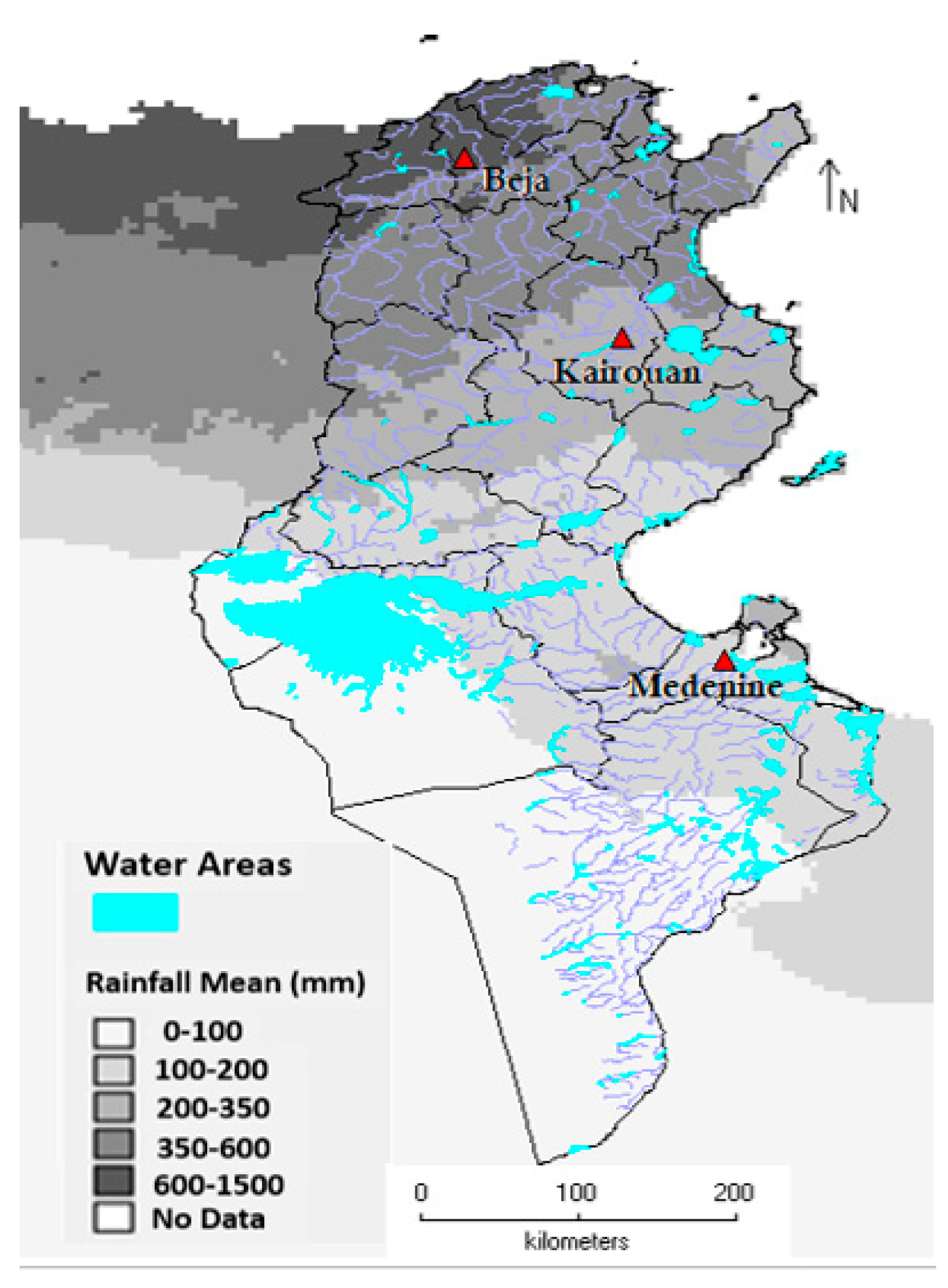
Description of Field Trial Sites

Field experiments were conducted during the 2012–2014 period in three contrasting locations (Beja, Kairouan, Medenine) of Tunisia. The Beja site (36°44′01.13″ N; 9°08′14.30″ E) is sub-humid, Kairouan (35°34′34.97″ N; 10°02′50.88″ E) is located in the semi-arid area of central Tunisia, and Medenine (33°26′54″ N, 10°56′31″ E) is part of the South East arid region of Tunisia (Figure 1). Two barley varieties (Konouz from Tunisia and Batini 100/1 B from Oman) were used for field experiments. The Konouz variety is salt-sensitive [29,30], whereas Batini 100/1 B is salt-tolerant [29,31].

In Kairouan (KAI) and Medenine (MED) field trial sites were divided into two sub-plots. Each subplot was irrigated by one water salinity treatment (EC = 2 and 13 dS m⁻¹). Three blocks were defined perpendicularly to the sub-plots so that both treatments were observed in each block. As Beja is located in the rainfed cereal growing area of Tunisia, no irrigation was applied.

The weather data characterize the trials sites related to temperature, and rain was described by [29]. The irrigation water applied and reference evapotranspiration (ET_o) registered in the trials during the two growing seasons are presented in

Table 1. Rainfall, irrigation water applied and evapotranspiration (ET_o) in three trial sites.

Growing Season	Rainfall (mm)			Irrigation Water Applied (mm)			ETo (mm)
	Sites			Sites			Sites
	Beja	KAI	MED	Beja	KAI	MED	Beja	KAI	MED
2012–2013	472.2	151.9	81.1	0	360	455	393.8	364.7	327.6
2013–2014	413.5	180.0	156.1	0	360	405	390.1	363.7	328.4

. The collected data from each site were used to estimate the reference evapotranspiration (ET) according to the Penman-Monteith Evapotranspiration FAO-56 Method, and then the total water supplied was determined for each site to obtain the water barley requirement. Irrigation was applied using a drip system. To ensure water supply homogeneity, line source emitters were installed at each planting row and 33-cm spacing between emitters on the same row.

Soil samples were taken from the trial sites, and physico-chemical analyses were performed. The site’s soil characteristics are diverse, from soil rich in clay and organic matter in BEJ to sandy soil with impoverished organic matter continent in MED (

Table 2. Soil properties in three field trial sites.

Site	Sand (%)	Clay (%)	Silt (%)	OM (%)	Na+ Content (ppm)	K+ Content (ppm)	Ca2+ Content (ppm)	PWP (% vol)	FC (% vol)
Beja	15.0	57.5	27.5	4.7	10–20	250–300	100–110	32.0	50.0
KAI	14.8	45.1	40.1	4.0	230–270	390–550	90–140	23.0	39.0
MED	55.5	20.5	24.0	0.9	120–200	30–70	30–55	6.0	13.0

(OM: organic matter, PWP: permanent wilting point; FC: field capacity).

).

Crops were sown during the last week of November. Seeds were hand sown at the rate of 200 viable grains per m². Nitrogen, potassium and phosphorus were applied separately at 85, 50, and 50 kg/ha rates, respectively.

At the five different stages, plants for each genotype, from three small areas (25 × 25 cm) were taken from each experimental unit and used to determine the biomass. At a final harvest stage, plot (1 × 2 m) was used for biomass and grain yield assessment. Water productivity (WP) was calculated as the ration between the collected yield expressed in kg ha⁻¹ and the daily transpiration simulated by the model.

3. Description of the AquaCrop Model

The model describes soil, water, crop, and atmosphere interactions through four sub-model components: (i) the soil with its water balance; (ii) the crop (development, growth, and yield); (iii) the atmosphere (temperature, evapotranspiration, and rainfall), and carbon dioxide (CO₂) concentration; and (iv) the management, such as irrigation and crop fertilization soil fertility.

The AquaCrop model is based on the relationship between the relative yield and the relative evapotranspiration [22] as follows

$$\frac{{\mathrm{Y}}_{\mathrm{x}}-{\mathrm{Y}}_{\mathrm{a}}}{{\mathrm{Y}}_{\mathrm{x}}}={\mathrm{K}}_{\mathrm{y}}\left(\frac{{\mathrm{ET}}_{\mathrm{x}}-{\mathrm{ET}}_{\mathrm{a}}}{{\mathrm{ET}}_{\mathrm{x}}}\right)$$

(1)

where Y_x is the maximum yield, Y_a is the actual yield, ET_x is the maximum evapotranspiration, ET_a is the actual evapotranspiration, and K_y is the yield response factor between the decrease in the relative yield and the relative reduction in evapotranspiration.

The AquaCrop model does not take into account the non-productive use of water for separating evapotranspiration (ET) into crop transpiration (T) and soil evaporation (E)

$$\mathrm{ET}=\mathrm{E}+\mathrm{Tr}$$

(2)

where ET = actual evapotranspiration, E = soil evaporation and Tr = the sweating of crop.

At a daily time step, the model successively simulates the following processes: (i) groundwater balance; (ii) development of green canopy (CC); (iii) crop transpiration; (iv) biomass (B); and (v) conversion of biomass (B) to crop yield (Y). Therefore, through the daily potential evapotranspiration (ET_o) and productivity of water (WP*), the daily transpiration (Tr) is converted into vegetal biomass as follows

$${\mathrm{B}}_{\mathrm{i}}={\mathrm{WP}}^{*}\left(\frac{{\mathrm{T}}_{\mathrm{ri}}}{{\mathrm{ETo}}_{\mathrm{i}}}\right)$$

(3)

where WP* is the normalized water productivity [32,33] relative to Tr. After the normalization of water productivity for different climatic conditions, its value can be converted into a fixed parameter [34]. The estimation and prediction of performance are based on the final biomass (B) and harvest index (HI). This allows a clear distinction between impact of stress on B and HI, in response to the environmental conditions

$$\mathrm{Y}=\mathrm{HI}\ast \left(\mathrm{B}\right)$$

(4)

where: Y = final yield; B = biomass; HI = harvest index.

During the calibration and testing of the model, we calculated water productivity (WP) as presented by Araya et al. [5]

$$\mathrm{WP}=\left[\frac{\mathrm{Y}}{\sum \mathrm{Tr}}\right]$$

(5)

where Y is the yield expressed in kg ha⁻¹ and Tr is the daily transpiration simulated by the model.

3.1. Crop Response to Soil Salinity Stress

The electrical conductivity of saturation soil-past extracts from the root zone (ECe) is commonly used as an indicator of the soil salinity stress to determine the total reduction in biomass production, determines the value for soil salinity stress coefficient (K_{s, salt}).

The coefficient of soil salinity stress (Ks_salt) varied between 0 (full effect of stress of soil salinity) and 1 (no effect). The following equation determined the reduction in biomass

B_rel = 100 (1 − Ks_salt)

(6)

B_rel represents the expected biomass production under given salinity stress relative to the biomass produced in the absence of salt stress. The coefficient is adjusted daily to the average ECe in the root zone [35].

Then, the thresholds values are given for the sensitive and tolerant barley genotype and expressed in dS m⁻¹. This allows the estimation of the lower limit (EC_en) to which the soil salinity stress begins to affect the production of biomass and the upper threshold (EC_ex), in which soil salinity stress has reached its maximum effect.

3.2. Soil Salinity Calculation

AquaCrop adopts the calculation procedure presented in BUDGET [36] to simulate the movement and retention of salt in the soil profile. The salts enter the soil profile as solutes after irrigation with saline water or through capillary rise from a shallow groundwater table (vertical downward and upward salt movement). The average ECe in the compartments of the effective rooting depth determines the effects of soil salinity on biomass production.

To explain the movement and retention of soil water and salts in the soil profile, AquaCrop divides the soil profile into 2 to 11 soil compartments called “cells”, depending on the type of soil in each horizon (clay, sandy horizon) and its saturated hydraulic conductivity (Ksat in mm/day). The salt diffusion between two adjacent cells (cell j and cell j+1) is determined by the differences in salt concentration and expressed by the electrical conductivity (EC) of soil water.

AquaCrop determines the vertical salt movement in response to soil evaporation, considering the amount of water extracted from the soil profile by evaporation and the wetness of the upper soil layer. The relative soil water content of the topsoil layer determines the fraction of the dissolved salts that moves with the evaporating water.

AquaCrop determines the vertical salt movement because of the capillary rise. Finally, the salt content of a cell is determined by

$${\mathrm{Salt}}_{\mathrm{cell}}=0.64{\mathrm{W}}_{\mathrm{cell}}{\mathrm{EC}}_{\mathrm{cell}}$$

(7)

Salt_cell is the salt content expressed in grams salts per m² soil surface, Wcell its volume expressed in liter per m² (1 mm = 1 L/m²), and 0.64 a global conversion factor used in AquaCrop to convert dS/m to g/L. The electrical conductivity of the soil water (ECsw) and of the electrical conductivity of saturation soil-past extract (ECe) at a particular soil depth (soil compartment) is calculated as

$${\mathrm{EC}}_{\mathrm{sw}}=\frac{{{\displaystyle \sum }}_{\mathrm{j}=1}^{\mathrm{n}}{\mathrm{Salt}}_{\mathrm{cell}.\mathrm{j}}}{0.64\left(1000\mathsf{\theta }{\Delta }_{\mathrm{z}}\right)\left\{1-\frac{{\mathrm{Vol}\%}_{\mathrm{gravel}}}{100}\right\}}$$

(8)

$${\mathrm{EC}}_{\mathrm{e}}=\frac{{{\displaystyle \sum }}_{\mathrm{j}=1}^{\mathrm{n}}{\mathrm{Salt}}_{\mathrm{cell}.\mathrm{j}}}{0.64\left(1000{\mathsf{\theta }}_{\mathrm{sat}}{\Delta }_{\mathrm{z}}\right)\left\{1-\frac{{\mathrm{Vol}\%}_{\mathrm{gravel}}}{100}\right\}}$$

(9)

where n is the number of cells in each soil compartment; θ is the soil water content (m³/m³); θ_sat is the soil water content (m³/m³) at saturation; Δz (m) is the thickness of the soil compartment and Vol% gravel is the volume percentage of the gravel in the soil horizon of each compartment.

4. Model Calibration

4.1. Input and Output Variables of the Model

The model was calibrated using data from the growing season of 2012–2013 and evaluated using data from 2013–2014. Determining parameters for crop development and production, as well as water and salinity stress, was fundamental for calibrating the AquaCrop model. The parameters of climate, soil, and crop management used for the model calibration are presented in

Table 3. Climate, soil and crop parameters used for the simulation model AquaCrop.

Climate		- Daily rainfall, daily ETo, daily temperatures
		- CO2 concentration
Crop	Limited set	Crop development and production parameters which include phenology and life cycle
	Crop parameters	- Harvest index
		- Root zone threshold at the end of the canopy expansion
		- Threshold root zone depletion for early senescence
		- Time for the maximum canopy cover
		- Maximum vegetation
		- Flowering time
		- Initial vegetative cover
		- Depletion threshold root zone for stomata closure
		- Extraction of water
	Field	- Soil fertility, mulch
		- Field practices (surface runoff presence, ground bond)
Soil	Soil profile	Characteristics of soil horizon (no of soil horizon, thickness, Permanent Wilting Point (PWP), Field Capacity (FC), Soil saturation (SAT), Ksat); soil surface (runoff, evaporation); Restrictive soil layer capillary rise).
	Soil water and groundwater	Constant depth; variable depth; water quality.

.

4.2. Statistical Parameters Used for the Calibration and Evaluation of Model

Several statistical indices were used to evaluate the performance of the model on the field measured data. These include Percentage Error (PE), Root Mean Square Error (RMSE), Model Efficiency (ME) and Coefficient of Determination (R²).

Percentage Error (PE) was determined using the following equation

$$\mathrm{EP}=\frac{\left({\mathrm{S}}_{\mathrm{i}}-{\mathrm{O}}_{\mathrm{i}}\right)}{{\mathrm{O}}_{\mathrm{i}}}\times 100$$

(10)

where S_i and O_i are simulated and observed values, respectively.

The root means square error (RMSE) [37] is presented by the following equation

$$\mathrm{RMSE}=\sqrt{\frac{1}{\mathrm{n}}{{\displaystyle \sum }}_{\mathrm{i}=1}^{\mathrm{n}}{\left({\mathrm{S}}_{\mathrm{i}}-{\mathrm{O}}_{\mathrm{i}}\right)}^2}$$

(11)

with the values of RMSE close to zero indicate the best model fit.

The model efficiency (ME) [38] was applied to assess the effectiveness of the model. The ME indicator compares the variability of prediction errors by the model to those of collected data from the field. If the prediction errors are greater than the data error, then the indicator becomes negative. The upper ME bound is at 1.

$$\mathrm{ME}=\frac{{{\displaystyle \sum }}_{\mathrm{i}=1}^{\mathrm{n}}{\left({\mathrm{O}}_{\mathrm{i}}-\mathrm{MO}\right)}^2–{{\displaystyle \sum }}_{\mathrm{i}=1}^{\mathrm{n}}{\left({\mathrm{S}}_{\mathrm{i}}-{\mathrm{O}}_{\mathrm{i}}\right)}^2}{{{\displaystyle \sum }}_{\mathrm{i}=1}^{\mathrm{n}}{\left({\mathrm{O}}_{\mathrm{i}}-\mathrm{MO}\right)}^2}$$

(12)

The coefficient of determination (R²), as a result of regression analysis, is the proportion of the variance in the dependent variable (predict value) that is predictable from the independent variable (observed value) and is computed according to [35]

$$\mathrm{R}²={\left\{\frac{{{\displaystyle \sum }}_{\mathrm{i}=1}^{\mathrm{n}}\left({\mathrm{O}}_{\mathrm{i}}-\overline{\mathrm{O}}\right)\left({\mathrm{S}}_{\mathrm{i}}-\overline{\mathrm{S}}\right)}{{\left[{{\displaystyle \sum }}_{\mathrm{i}=1}^{\mathrm{n}}{({\mathrm{O}}_{\mathrm{i}}-\overline{\mathrm{O}})}^2\right]}^{0.5}{\left[{{\displaystyle \sum }}_{\mathrm{i}=1}^{\mathrm{n}}{({\mathrm{S}}_{\mathrm{i}}-\overline{\mathrm{S}})}^2\right]}^{0.5}}\right\}}^2$$

(13)

R² is between 0 and 1.

4.3. Parameters Used for Model Calibration

In total, 26 input parameters were used for the model calibration (

Table 4. Final values of different model input parameters obtained after calibration for two genotypes under different salinity levels (S1 = 2 dS m⁻¹; S2 = 13 dS m⁻¹).

		Batini-100/1 B (Salt-Tolerant)			Konouz (Salt-Sensitive)			Remarks
		BEJ	KAI	MED	BEJ	KAI	MED
Base temperature (°C)	S1	0	0	0	0	0	0	Conservative
	S2	-	0	0	-	0	0
Upper temperature (°C)	S1	30	30	30	30	30	30	Conservative
	S2	-	30	30	-	30	30
Initial canopy cover, CC0 (%)	S1	1.5	1.5	1.5	1.5	1.5	1.5	Conservative
	S2	-	1.5	1.5	-	1.5	1.5
Canopy cover per seeding (cm2/plant)	S1	0.75	0.75	0.75	0.75	0.75	0.75	Conservative
	S2	-	0.75	0.75	-	0.75	0.75
Maximum coefficient for transpiration, KcTr, x	S1	0.90	0.90	0.90	0.90	0.90	0.90	Conservative
	S2	-	0.90	0.90	-	0.90	0.90
Maximum coefficient for soil evaporation, Kex	S1	0.4	0.4	0.4	0.4	0.4	0.4	Conservative
	S2	-	0.4	0.4	-	0.4	0.4
Upper threshold for canopy expansion, Pexp, upper	S1	0.30	0.30	0.30	0.20	0.20	0.20	Varietal effect
	S2	-	0.30	0.30	-	0.20	0.20
Lower threshold for canopy expansion, Pexp, lower	S1	0.65	0.65	0.65	0.55	0.55	0.55	Varietal effect
	S2	-	0.65	0.65	-	0.55	0.55
Leaf expansion stress coefficient curve shape	S1	4.5	4.5	4.5	4.5	4.5	4.5	Conservative
	S2	4.5	4.5	4.5	4.5	4.5	4.5
Upper threshold for stomatal closure, Psto, upper	S1	0.6	0.6	0.6	0.55	0.55	0.55	Varietal effect
	S2	-	0.6	0.6	-	0.55	0.55
Leaf expansion stress coefficient curve shape	S1	4.5	4.5	4.5	4.5	4.5	4.5	Conservative
	S2	4.5	4.5	4.5	4.5	4.5	4.5
Canopy senescence stress coefficient, Psen, upper	S1	0.65	0.65	0.65	0.55	0.45	0.45	Varietal effect and site effect for the sensitive
	S2	-	0.65	0.65	-	0.45	0.45
Senescence stress coefficient curve shape	S1	4.5	4.5	4.5	4.5	4.5	4.5	Conservative
	S2	4.5	4.5	4.5	-	4.5	4.5
Reference harvest index, HI0 (%)	S1	40	40	41	41	42	45	Varietal and salt stress effect
	S2		40	45		41	41
Normalized crop water productivity, WP* (g/m2)	S1	14	14	14	14	14	14	Conservative
	S2	14	14	14	14	14	14
Time from sowing to emergence (day)	S1	7	7	7	7	7	7	Conservative
	S2	7	7	7	7	7	7
Time from sowing to maximum CC (jours)	S1	60	60	60	62	60	57	Varietal and salt stress effect
	S2	-	60	58	-	59	55
Time from sowing to maximum CC (day)	S1	145	145	145	145	145	145	Conservative
	S2	-	145	145	145	145	145
Time from sowing to maturity (day)	S1	178	157	157	178	157	157	Varietal and salt stress effect
	S2	-	157	157	-	157	157
Maximum canopy cover, CCx (%)	S1	87	87	87	87	75	63	Varietal and salt stress effect
	S2	-	87	70	-	60	40
Canopy growth coefficient, CGC (%/day)	S1	12.5	12.5	12.5	12	12	12	Varietal effect
	S2		12.5	12.5		12	12
Canopy decline coefficient, CDC (%/day)	S1	6	6	6	6	6	6	Conservative
	S2	-	6	6	-	6	6
Maximum effective rooting depth, Zx (m)	S1	0,9	0.75	0.75	0,9	0.75	0.75	Site effect
	S2	-	0.75	0.75	-	0.75	0.75
Salinity stress, lower threshold, ECen (dS m−1)	S1	3	3	3	1	1	1	Varietal effect
	S2	3	3	3	1	1	1
Salinity stress, upper threshold, ECex (dS m−1)	S1	22	22	22	18	18	18	Varietal effect
	S2	22	22	22	18	18	18
Shape factor for salinity stress coefficient curve	S1	1	1	1	1	1	1	Conservative
	S2	1	1	1	1	1	1

For Bej only rainfall; for Kai, two levels of water salinity (S1 = 1.2 dS m⁻¹; S2 = 13 dS m⁻¹ (S2)); for Med, two levels of water salinity (S1 = 2 dS m⁻¹; S2 = 13 dS m⁻¹ (S2)).

). Out of these, 14 parameters were considered as “conservative” because they do not change with salinity and are independent of limiting or non-limiting conditions. These parameters include normalized crop water productivity and crop transpiration coefficient. The remaining 12 are site-specific (climate, water, and soil salinity) and crop-specific (tolerant or sensitive). These input parameters were adjusted during the calibration process to obtain better adequacy between the measured and simulation values.

4.4. Development of Different Scenarios

After calibration and evaluation, the model was used to assess the performance of two barley varieties under three water salinity conditions scenarios i.e., 5, 10, and 15 dS m⁻¹, using the weather data for the growing season 2013–2014.

4.5. The Economic Gain from the Use of a Unit of Water Consumed in the Tow Barley Varieties under Different Climatic Conditions

The economic productivity of two barley varieties was estimated using the average unit cost of one water cubic meter in Tunisia and the water use predicted by AquaCrop. The crop water economic productivity of the tolerant and the sensitive barley varieties as the measure of the biophysical and then economic gain from the use of a unit of water consumed were estimated by AquaCrop model in grain yield production [20]. This is expressed in productive crop units of kg/m³ and money unit/m³.

5. Results

5.1. Biophysical Environments Variability of Experimental Sites

The experiments are conducted in adaptability trials set up in three contrasting biophysical environments (from the sub-humid to the arid interior). These sites, namely Beja, Kairouan and Medenine, were selected on a North–South transect (Figure 1). The soils of the trial sites are very diverse, from soil rich in clay and poor in organic matter in BEJ to sandy soil with poor organic matter continent in MED (Table 2). Beja’s sub-humid site received annual rainfall of 472 and 413 mm respectively during the two cropping seasons. However, in the semi-arid and arid sites, low rainfall was registered. The arid site of MED received an annual rainfall of 81 mm during the first cropping season and 156 mm during the second. At Kairouan, the rainfall for the 2012/2013 and 2013/2014 seasons was 152 and 180 mm, respectively (Table 1). As Beja is located in the rainfed cereal-growing area of Tunisia, no irrigation was applied. KAI and MED field trial sites, two different salinities (EC = 2 and 13 dS m⁻¹) of water were used for irrigation.

Soil calcium and potassium content was higher in KAI as compared to MED. Soil sodium content changes during the different experimentation period following irrigation with saline water in KAI and MED, where sodium is the dominant element present in the saline irrigation water. The variation between sites might be explained by the variation in the cationic exchange capacity of the sandy soil and torrential character of the rainfall in this area (Table 2).

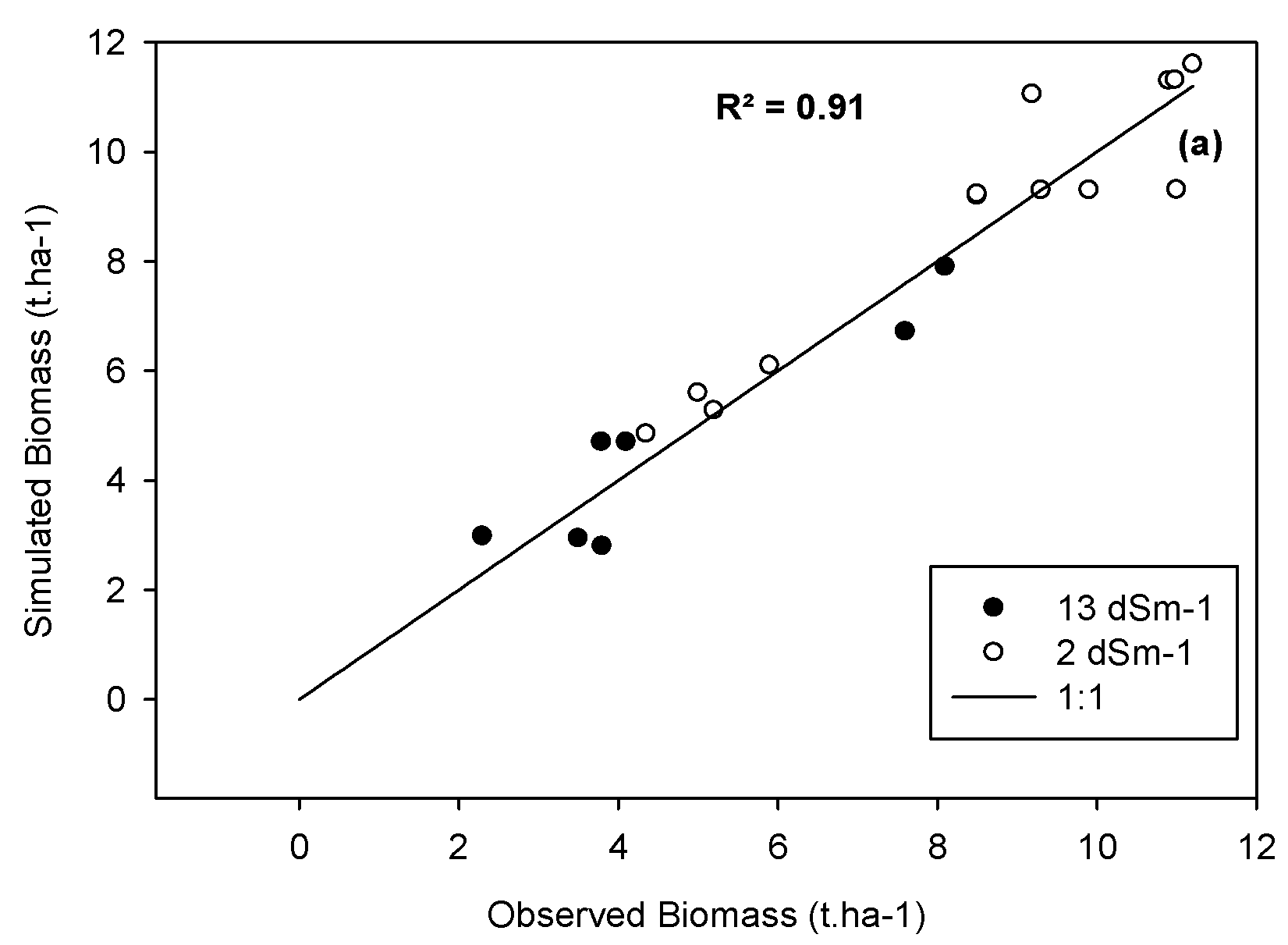
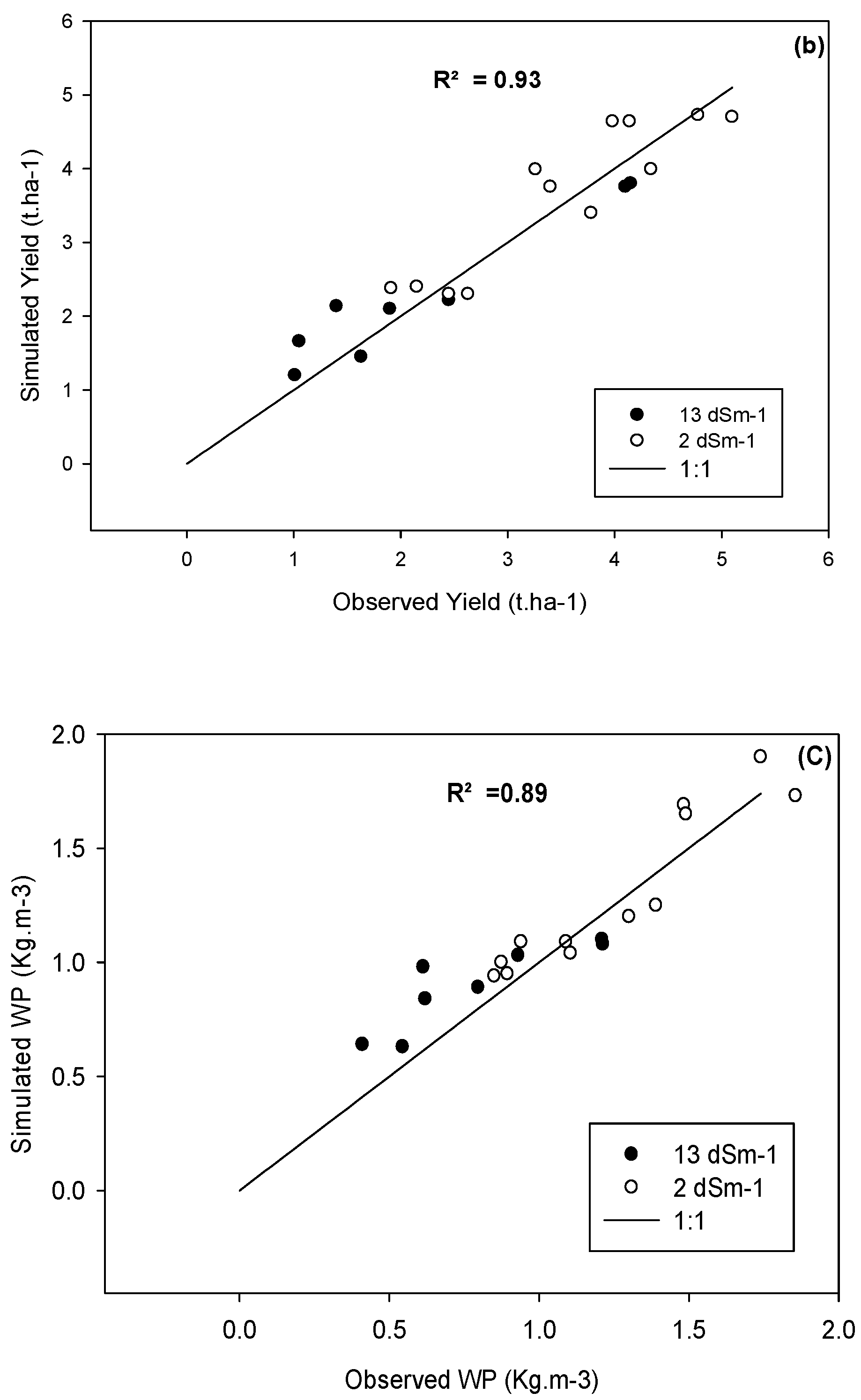
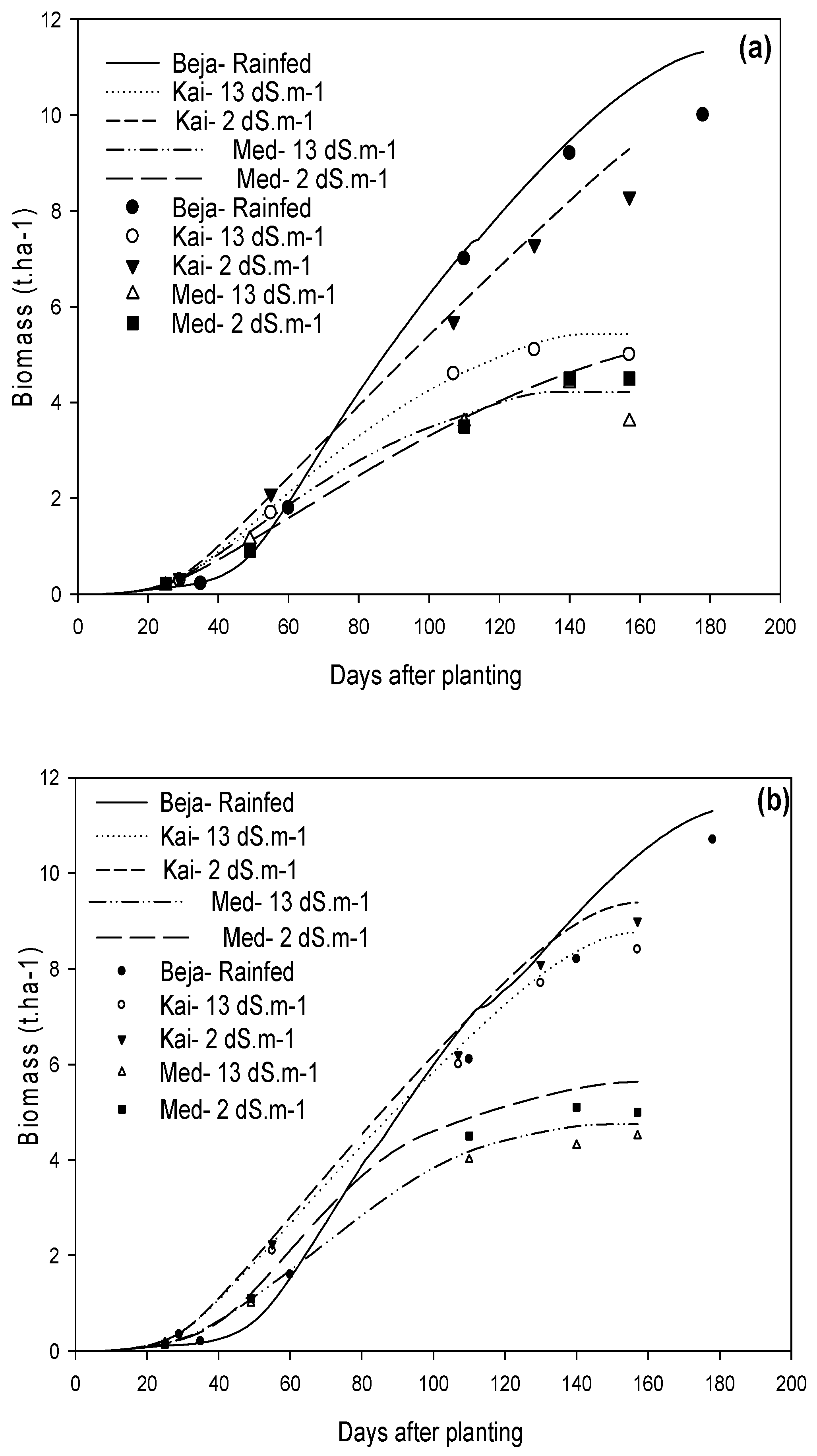
5.2. Biomass, Grain Yield, and Water Use Efficiency

The correlation between grain yield, biomass, and water productivity values for two barley genotypes showed that the observed and simulated values are closely co-related, as evidenced by the high R² values, i.e., 0.91, 0.93, and 0.89 for grain yield, biomass, and water productivity, respectively (Figure 2).

The correlation between observed and simulated values of biomass yield for two barley genotypes at three locations showed proximity (Figure 3), which indicates the excellent ability of the AquaCrop model to predict biomass yield under different agro-climatic conditions. The results also show that the sensitive barley variety at MED produces the lowest biomass for both irrigation water qualities. Similar trends were observed for grain yield, where the tolerant barley variety performed better than the sensitive variety regardless of the location and the quality of irrigation water.

5.3. Canopy Cover (CC)

The maximum and minimum CC were 85% and 30% in the sub-humid and arid areas, respectively. The salinity induces a 10% reduction in the CC in the sub-humid environment and 5–30% in the dry climate of MED. CC reduction under saline irrigation water is less noticeable in the tolerant variety than the sensitive variety for both salinity levels. However, in the rainfed area of Beja, the growth of both varieties was comparable.

Figure 4 shows a strong correlation between measured and simulated CC values for both varieties of barley (R² = 0.91 and R² = 0.93). In general, a good match between the observed and the simulated CC was observed in all three locations. However, the model somewhat over-estimated CC in the rainfed environment of Beja and slightly under-estimated it in the other two situations.

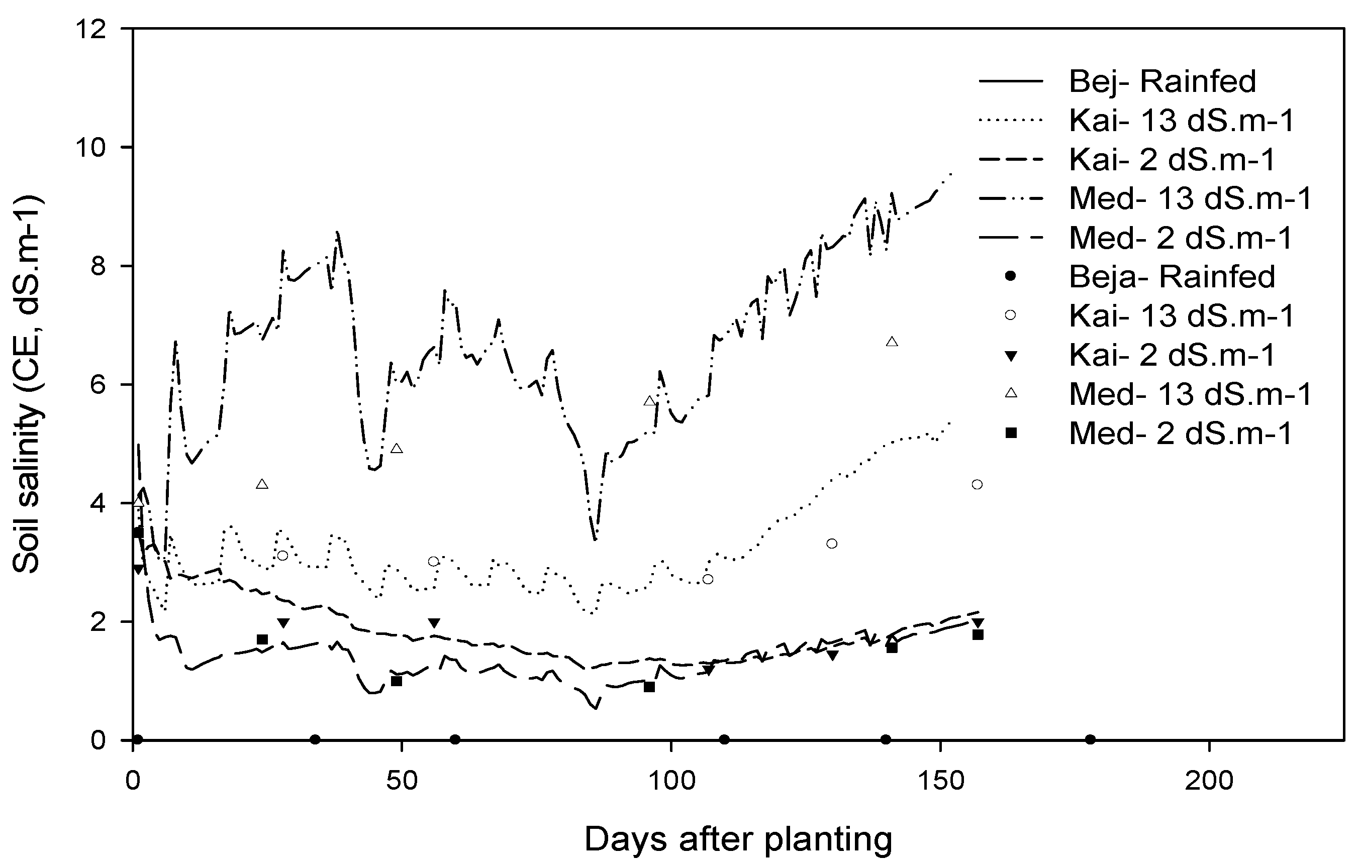
5.4. Effects of Soil Salinity

The maximum soil salinity was in the arid and semi-arid areas irrigated with saline water, respectively. The soil salinisation dynamic depends on the salinity of irrigation water. However, in the rainfed area of Beja, we noted the absence of any salty issue.

Figure 5 shows that the simulated soil salinity trend in the root zone (up to a depth of 0.7 m) corresponds very well with the measured values under different saline water regimes across different environments throughout the growing season. The observed and modeled soil salinity correlated well, with an R² of 0.96. Figure 5 shows that the model reliably simulated average root zone salinity when the crop is irrigated with low-salinity water (2 dS m⁻¹). However, it slightly underestimated soil salinity under higher saline water conditions (13 dS m⁻¹), particularly for the late growing season.

5.5. Statistical Indices for AquaCrop Model Evaluation

The statistical indices derived for evaluating the AquaCrop model’s performance in predicting soil water content, yield, canopy cover percent, biomass, and water productivity (WP) of barley genotypes under different saline water regimes across different environments are given in

Table 5. Statistical indices values for different parameters obtained for model calibration.

	Variable	RMSE	ME	R2
Calibration	Grain yield (t ha−1)	0.40	0.89	0.91
	Biomass (t ha−1)	0.87	0.96	0.93
	water productivity (kg ha−1 mm−1)	0.15	0.84	0.89
	Soil salinity	0.34	0.91	0.95
	Canopy cover percent	1.5	0.89	0.91
Evaluation	Grain yield (t ha−1)	0.45	0.87	0.89
	Biomass (t ha−1)	0.89	0.86	0.87
	water productivity (kg ha−1 mm−1)	0.13	0.91	0.84
	Soil salinity	1.25	0.91	0.96
	Canopy cover percent	2.25	0.89	0.91

. All statistical parameters depict a strong correlation between simulated and observed values for model calibration and evaluation periods. The correlation between all statistical parameters remained almost the same for the calibration and evaluation period, which indicates the robustness of the model prediction. Based on the model calibration and evaluation results, the model was found robust enough to calculate different scenarios.

6. Development of Different Scenarios

Due to a shortage of surface water, farmers of KAI and MED regions have no option than to use groundwater for irrigation. The quality of groundwater ranges from 4 to15 dS m⁻¹ in these two regions. Farmers are interested to know which barley varieties would be most suitable to grow under these groundwater quality conditions. The calibrated and evaluated model was used to assess the performance of two barley varieties under three water salinity conditions i.e., 5, 10, and 15 dS m⁻¹, and the results are presented in

Table 6. Predicted values of biomass, yield, and water productivity of two barley varieties for different scenarios.

	BEJ	KAI			MED
	Rainfed	5 dS m−1	10 dS m−1	15 dS m−1	5 dS m−1	10 dS m−1	15 dS m−1
Tolerant genotype
Biomass (t ha−1)	11.30	9.07	8.36	5.48	5.60	4.74	4.70
Yield (t ha−1)	4.70	3.65	3.44	2.20	2.29	2.13	2.10
WP (kg m−3)	1.73	1.29	1.19	0.85	1.25	1.18	1.00
Sensitive genotype
Biomass (t ha−1)	11.33	6.62	4.60	1.90	3.18	3.03	2.80
Yield (t ha−1)	4.64	2.70	1.90	0.80	1.40	1.30	0.80
WP (kg m−3)	1.65	1.12	0.85	0.45	0.74	0.72	0.51

.

The performance of both barley varieties in the KAI area is predicted to be much higher than MED area under all salinity levels due to prevailing climatic conditions. In the KAI area, biomass and grain yield reductions are much higher with the increasing water salinity for both varieties. For example, the biomass and yield reductions in the KAI area were about 40%with an increase in salinity from 5 to 10 and 15 dS m⁻¹. For the sensitive genotype, the biomass and yield reductions in the KAI area would be above 72% with a similar increase in the salinity levels. Although overall biomass and grain yields in the MED area were lower than in the KAI area, biomass and yield reductions for the salt-tolerant barley variety were only 16% and 8%, with an increase in salinity from 5 to 15 dSm⁻¹, respectively. However, for the sensitive genotype, reductions in biomass and yield were 12% and 43%, respectively, with a similar increase in salinity levels. Similar trends are obtained for water productivities.

Without salt stress, both varieties have the same performance. However, the tolerant variety performs better than the sensitive variety under salt stress. This is because it has better potential. Therefore, farmers can grow both varieties in the rainfed areas of BEJ, while, in KAI and MED areas where irrigation is necessary for crop growth, the salt-tolerant barley variety should be preferred. The cultivation of the salt-sensitive barley variety in the MED area will be risky, as the yields will be low, and the development of soil salinity over time will remain a challenge. This situation will be very critical for long-term sustainable crop production in the area.

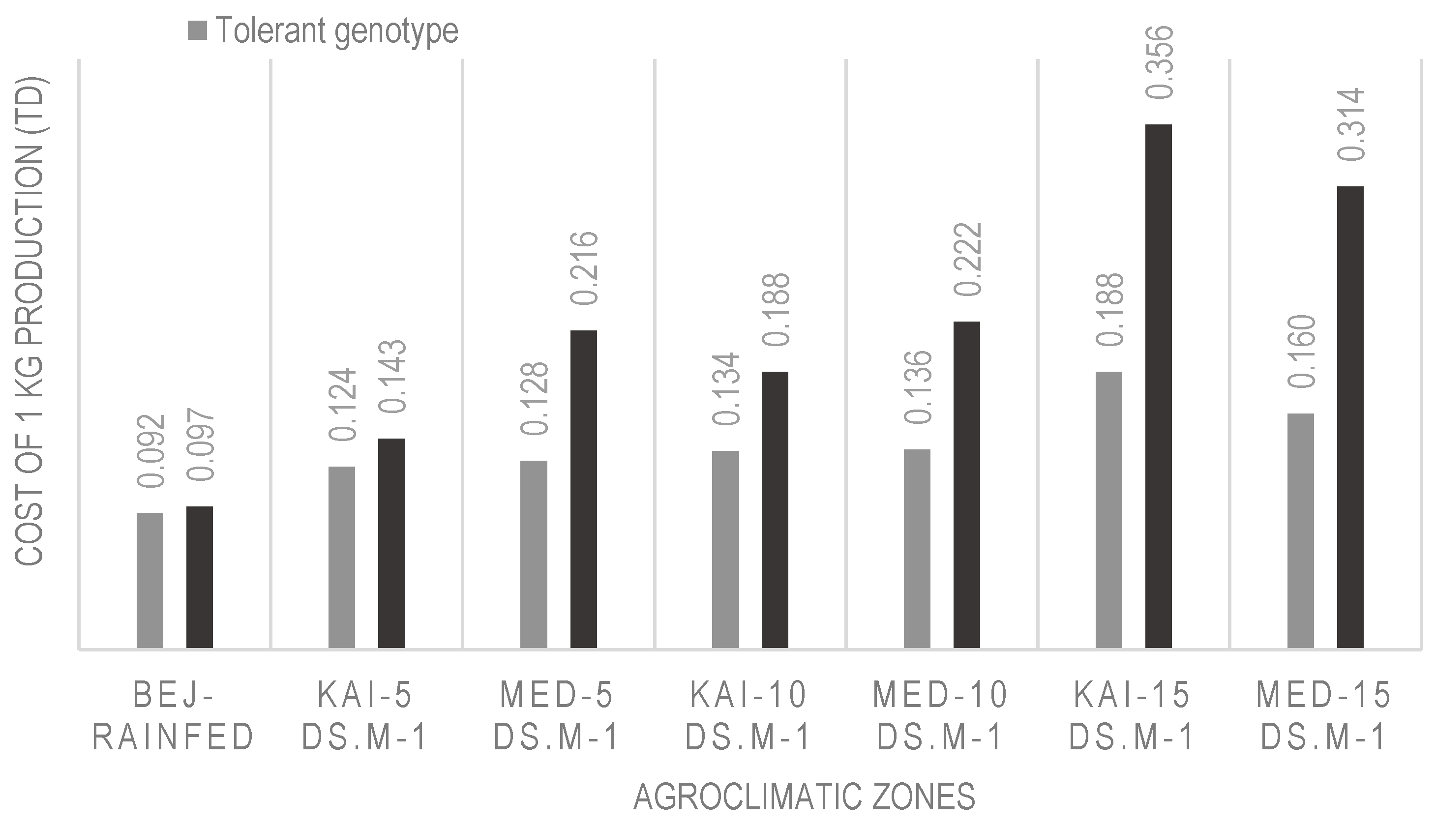
7. Economic Productivity of Barley Varieties under Different Climatic Conditions

The economic productivity of two barley varieties was estimated using the average unit cost of one water cubic meter in Tunisia and the water use predicted by AquaCrop. The results show that the production cost of 1 kg of barley is lowest in the BEJ area compared to those areas where it is irrigated with saline water.

In the KAI region, the cost will be reduced by 13.28% 28.72% and 47.19% by growing the tolerant variety irrigated with saline water of 5, 10, and 15 dS m⁻¹, respectively. In the arid region of MED, the benefit will be reduced by 40%, 38%, and 49% by growing the tolerant barley variety by irrigating with saline water of 5, 10 and 15 dS m⁻¹, respectively (Figure 6). However, in the sub-humid region of BEJ, there is no significant difference between susceptible and tolerant genotypes. The results show the economic interest for arid region farmers to grow the tolerant barley variety. This stresses the need for appropriate breeding programs for the saline environments for optimizing crop production instead of targeting potential yields.

8. Discussion

We evaluated the AquaCrop model for two barley varieties under contrasting environments and different water salinity levels. The simulated model values were close to the field measurements concerning biomass, yield and soil salinity. ME and R² parameters were close to 0.9, showing the model’s ability to simulate the behavior of sensitive and resistant cultivars in contrasting environments and irrigation practices. Araya et al. [5] reported R² values of 0.80 when simulating barley biomass and grain yield using AquaCrop. El Mokh et al. [25] reported R² values of 0.88 when simulating barley yield under different irrigation regimes in a dry environment using AquaCrop. Mondal et al. [24] reported a 0.12 t ha⁻¹ root mean square error after simulating the yield response of rice to salinity stress with the AquaCrop model. Our results also show a correct prediction with an RMSE of 0.45 t ha⁻¹ (Table 5). This shows that the AquaCrop model simulates biomass production for all environments with an acceptable accuracy level.

AquaCrop model produces consistent simulation results for CC with an R² of 0.89 and RMSE of 2.25 (Table 5). The model also simulated soil salinity satisfactorily for all environments (R² = 0.96) for all situations. The R² values exceeding 0.8 are considered excellent for model performance [39]. The ability of AquaCrop to predict yield depends on the appropriate calibration of the canopy cover curve [1,40]. Indeed, after simulation of soil water balance at a daily time step, the model simulates CC and then simulates the transpiration of a crop, biomass above the soil, and converts biomass into yield. Therefore, it is essential to make accurate predictions of the canopy cover by the proper calibration of crop traits.

Therefore, through proper calibration, models can be used for additional solutions for the quantification of salinity build-up in the root zone [41].

We also noted the overestimation of the soil salinity at the end of the growing season when saline water is used for irrigation (Figure 5). This could be due to the excessive leaching of salts from the soil profile through irrigation, as reported by Mohammadi et al. [42]. Over- or underestimation at the end of the season could be the simplification of soil salt transport calculations in the model based on some empirical functions, including the parameters of Ks and the drainage coefficient for vertical downward salt movement. Furthermore, the occasional leaching of salts from the root zone using relatively better-quality water is also recommended. Changing cropping patterns is also a useful strategy for the rehabilitation and management of saline soils, especially when only saline water is available for irrigation.

The AquaCrop model was also capable of predicting water productivity under sub-humid, semi-arid, and arid environments and the effect of salinity. Plants subjected to salinity stress show a varying response in WP. The sensitive genotype was more exposed to varying responses in WP. Besides, heat stress induced by increased temperatures and the water deficit also decreases productivity, as demonstrated by Hatfield [43]. The observed and predicted water productivities were directly affected by climate aridity and the salinity of the irrigation water. However, the tolerant barley variety was less affected by these factors. These results are in agreement with the earlier studies [16,44].

Water scarcity is already hampering agricultural production in the MENA region. Therefore, the adoption of integrated management strategies will be useful for growing tolerant genotypes under saline water conditions and increasing the water use efficiency. For the sustainable management of crop growth in saline environments, soil-crop-water management interventions consistent with site-specific conditions need to be adopted [41]. These may include cyclic or conjunctive saline water use and freshwater through proper irrigation scheduling to avoid salinity development.

There are several traits available for screening genetic material for enhanced production and WP under different climate scenarios. This study shows that, under different water salinity conditions, sensitive barley genotype is more affected by the increasing water salinity than the tolerant barley genotype. The crop yields for both genotypes under all water salinity levels were higher in KAI area compared to the MED area. Therefore, this study recommends that farmers with higher salinity water for irrigation should grow tolerant barley genotypes, allowing them to reduce the cost, on average, by 30% (Figure 6). However, from a sustainability point of view, irrigation amounts should be kept to a minimum to optimize crop yields instead of targeting potential yields [45]. This exercise will help there be less accumulation of salts in the root zone. Besides, the occasional leaching of salts from the root zone using relatively better-quality water is also recommended. Changing cropping patterns is also regarded as a useful strategy for the rehabilitation and management of saline soils, especially when only saline water is available for irrigation [46,47].

9. Conclusions

The AquaCrop model with a salinity module was used to evaluate the agronomic performance of two barley varieties for the three different agro-climatic zones in Tunisia. These zones represent sub-humid, semi-arid, and arid climates. The model was calibrated and evaluated using field data from two years (2012 and 2014). The excellent correlation between the simulated and measured data of biomass, yield, and soil salinity confirms the ability of AquaCrop model to simulate crop growth under different climatic conditions. The scenario results using the calibrated model indicate that farmers with higher salinity water for irrigation should grow tolerant barley genotypes. However, from a sustainability point of view, irrigation amounts should be kept to a minimum to optimize crop yields instead of targeting potential yields.

References

1. Abi Saab, M.T.; Albrizio, R.; Nangia, V.; Karam, F.; Rouphael, Y. Developing scenarios to assess sunflower and soybean yield under different sowing dates and water regimes in the Bekaa valley (Lebanon): Simulations with Aquacrop. Int. J. Plant Prod. 2014, 8, 457–482. [Google Scholar]
2. Ahmed, M.; Goyal, M.; Asif, M. Silicon the non-essential beneficial plant nutrient to enhanced drought tolereance in wheat. In Crop Plant; Goyal, A., Ed.; Intech Publication House: London, UK, 2012; pp. 31–48. [Google Scholar]
3. Andarzian, B.; Bannayan, M.; Steduto, P.; Mazraeh, H.; Barati, M.E.; Barati, M.A.; Rahnama, A. Validation and testing of the AquaCrop model under fulland deficit irrigated wheat production in Iran. Agric. Water Manag. 2011, 100, 1–8. [Google Scholar] [CrossRef]
4. Araya, A.; Habtub, S.; Hadguc, K.; Kebedea, A.; Dejened, T. Test of AquaCrop model in simulating biomass and yield of water deficient and irrigated barley (Hordeum vulgare). Agric. Water Manag. 2010, 97, 1838–1846. [Google Scholar] [CrossRef]
5. Araya, A.; Keesstra, S.D.; Stroosnijder, L. Simulating yield response to water of Tef (Eragrostistef) with FAO’s AquaCrop model. Field Crop. Res. 2010, 116, 1996–2204. [Google Scholar] [CrossRef]
6. Chauhdarya, J.N.; Bakhsh, A.; Ragab, R.; Khaliq, A.; Bernard, A.; Engeld, M.R.; Shahid, M.N.; Nawaz, Q. Modeling corn growth and root zone salinity dynamics to improve irrigation and fertigation management under semi-arid conditions. Agric. Water Manag. 2020, 230, 105952. [Google Scholar] [CrossRef]
7. FAO (Food and Agriculture Organization of the United Nations). Advances in the Assessment and Mmonitoring of Salinization and Status of Biosaline Agriculture; FAO: Rome, Italy, 2010. [Google Scholar]
8. Qadir, M.; Quillérou, E.; Nangia, V.; Murtaza, G.; Singh, M.; Thomas, R.J.; Drechsel, P.; Noble, A.D. Economics of salt-induced land degradation and restoration. Nat. Resour. Forum 2014, 38, 282–295. [Google Scholar] [CrossRef]
9. Hatfield, J.L.; Dold, C. Water-Use efficiency: Advances and challenges in a changing climate. Front. Plant Sci. 2019. [Google Scholar] [CrossRef] [Green Version]
10. Zhou, G.; Johnson, P.; Ryan, P.R. Quantitative trait loci for salinity tolerance in barley (Hordeum vulgare L.). Mol. Breed. 2012, 29, 427–436. [Google Scholar] [CrossRef]
11. Newton, A.C.; Flavell, A.J.; George, T.S.; Leat, P.; Mullholland, B.; Ramsay, L.; RevoredoGiha, C.; Russell, J.; Steffenson, B.J.; Swanston, J.S.; et al. Crops that feed the world 4. Barley: A resilient crop? Strengths and weaknesses in the context of food security. Food Secur. 2011, 3, 141–178. [Google Scholar] [CrossRef]
12. Zhang, H.; Han, B.; Wang, T.; Chen, S.; Li, H.; Zhang, Y.; Dai, S. Mechanisms of Plant Salt Response: Insights from Proteomics. J. Proteome Res. 2012, 11, 49–67. [Google Scholar] [CrossRef]
13. Negrao, S.; Schmockel, S.M.; Tester, M. Evaluating physiological responses of plants to salinity stress. Ann. Bot. 2017, 119, 1–11. [Google Scholar] [CrossRef] [PubMed] [Green Version]
14. Heng, L.K.; Hsiao, T.; Evett, S.; Howell, T.; Steduto, P. Validating the FAO AquaCrop model for irrigated and water deficient field maize. Agron. J. 2009, 101, 488–498. [Google Scholar] [CrossRef] [Green Version]
15. Verma, A.K.; Gupta, S.K.; Isaac, R.K. Use of saline water for irrigation in monsoon climate and deep water table regions: Simulation modelling with SWAP. Agric. Water Manag. 2012, 115, 186–193. [Google Scholar] [CrossRef]
16. Soothar, R.K.; Wenying, Z.; Yanqing, Z.; Moussa, T.; Uris, M.; Wang, Y. Evaluating the performance of SALTMED model under alternate irrigation using saline and fresh water strategies to winter wheat in the North China Plain. Environ. Sci. Pollut. Res. 2019, 26, 34499–34509. [Google Scholar] [CrossRef] [PubMed]
17. Steduto, P.; Hsiao, T.C.; Raes, D.; Fereres, E. AquaCrop—The FAO crop model to simulate yield response to water. I. Concepts and underlying principles. Agron. J. 2009, 101, 426–437. [Google Scholar] [CrossRef] [Green Version]
18. Van Gaelen, H. AquaCrop Training Handbooks–Book II Running AquaCrop; Food and Agriculture Organization of the United Nations: Rome, Italy, 2016. [Google Scholar]
19. Doorenbos, J.; Kassam, A.H. Yield Response to Water; FAO Irrigation and Drainage Paper No. 33; FAO: Rome, Italy, 1979. [Google Scholar]
20. Kumar, A.; Sarangi, D.K.; Singh, R.; Parihar, S.S. Evaluation of aquacrop model in predicting wheat yield and water productivity under irrigated saline regimes. Irrig. Drain. 2014, 63, 474–487. [Google Scholar] [CrossRef]
21. Mondal, M.S.; Fazal, M.A.; Saleh, M.D.; Akanda, A.R.; Biswas, S.K.; Moslehuddin, Z.; Sinora, Z.; Attila, N. Simulating yield response of rice to salinity stress with the AquaCrop model. Environ. Sci. Process. Impacts 2015, 17, 1118–1126. [Google Scholar] [CrossRef] [Green Version]
22. El Mokh, F.; Nagaz, K.; Masmoudi, M.M.; Mechlia, N.B.; Fereres, E. Calibration of AquaCrop Salinity Stress Parameters for Barley under Different Irrigation Regimes in a Dry Environment; Springer: Cham, Germany, 2017. [Google Scholar] [CrossRef]
23. Hellal, F.; Mansour, H.; Mohamed, A.H.; El-Sayed, S.; Abdelly, C. Assessment water productivity of barley varieties under water stress by AquaCrop model. AIMS Agric. Food 2019, 4, 501–517. [Google Scholar] [CrossRef]
24. Tan, S.; Wang, Q.; Zhang, J.; Chen, Y.; Shan, Y.; Xu, D. Performance of AquaCrop model for cotton growth simulation under film-mulched drip irrigation in southern Xinjiang, China. Agric. Water Manag. 2018, 196, 99–113. [Google Scholar] [CrossRef]
25. Hammami, Z.; Gauffreteau, A.; BelhajFraj, M.; Sahlia, A.; Jeuffroy, M.H.; Rezgui, S.; Bergaoui, K.; McDonnell, R.; Trifa, Y. Predicting yield reduction in improved barley (Hordeum vulgare L.) varieties and landraces under salinity using selected tolerance traits. Field Crop. Res. 2017, 211, 10–18. [Google Scholar] [CrossRef]
26. Sbei, H.; Sato, K.; Shehzad, T.; Harrabi, M.; Okuno, K. Detection of QTLs for salt tolerance in Asian barley (Hordeum vulgare L.) by association analysis with SNP markers. Breed. Sci. 2014, 64, 378–388. [Google Scholar] [CrossRef] [PubMed] [Green Version]
27. Jaradat, A.A.; Shahid, M.; Al-Maskri, A.Y. Genetic diversity in the Batini barley landrace from Oman: Spike and seed quantitative and qualitative traits. Crop. Sci. 2014, 44, 304–315. [Google Scholar] [CrossRef]
28. Raes, D.; Steduto, P.; Hsiao, T.C.; Fereres, E. Crop Water Productivity. Calculation Procedures and Calibration Guidance. AquaCrop Version 3.0. FAO; Land and Water Development Division: Rome, Italy, 2009. [Google Scholar]
29. Trombetta, A.; Iacobellis, V.; Tarantino, E.; Gentile, F. Calibration of the AquaCrop model for winter wheat using MODIS LAI images. Agric. Water Manag. 2015, 164. [Google Scholar] [CrossRef]
30. Hanks, R.J. Yield and water-use relationships. In Limitations to Efficient Water Use in Crop Production; Taylor, H.M., Jordan, W.R., Sinclair, T.R., Eds.; ASA, CSSA, and SSSA: Madison, WI, USA, 1983; pp. 393–411. [Google Scholar]
31. Tanner, C.B.; Sinclair, T.R. Efficient water use in crop production: Research or re-search? In Limitations to Efficient Water Use in Crop Production; Taylor, H.M., Jordan, W.R., Sinclair, T.R., Eds.; ASA, CSSA, and SSSA: Madison, WI, USA, 1983; pp. 1–27. [Google Scholar]
32. Steduto, P.; Hsiao, T.C.; Fereres, E. On the conservative behavior of biomass water productivity. Irrig. Sci. 2007, 25, 189–207. [Google Scholar] [CrossRef] [Green Version]
33. Raes, D.; Steduto, P.; Hsiao, T.C.; Fereres, E. AquaCrop Version 5.0 Reference Manual; Food and Agriculture Organization of the United Nations: Rome, Italy, 2016. [Google Scholar]
34. Loague, K.; Green, R.E. Statistical and graphical methods for evaluating solute transport models: Overview and application. J. Contam. Hydrol. 1991, 7, 51–73. [Google Scholar] [CrossRef]
35. Minhas, P.S.; Tiago, B.; AlonBen-Gal, R.; Pereira, L.S. Coping with salinity in irrigated agriculture: Crop evapotranspiration and water management issues. Agric. Water Manag. 2020, 227, 105832. [Google Scholar] [CrossRef]
36. Pereira, L.S.; Paredes, P.; Rodrigues, G.C.; Neves, M. Modeling barley water use and evapotranspiration partitioning in two contrasting rainfall years. Assessing SIMDualKc and AquaCrop models. Agric. Water Manag. 2015, 159, 239–254. [Google Scholar] [CrossRef]
37. Iqbal, M.A.; Shen, Y.; Stricevic, R.; Pei, H.; Sun, H.; Amiri, E.; Rio, S. Evaluation of FAO Aquacrop model for winter wheat on the North China plain under deficit from field experiment to regional yield simulation. Agric. Water Manag. 2014, 135, 61–72. [Google Scholar] [CrossRef]
38. Mohammadi, M.; Ghahraman, B.; Davary, K.; Ansari, H.; Shahidi, A.; Bannayan, M. Nested validation of AquaCrop model for simulation of winter wheat grain yield soil moisture and salinity profiles under simultaneous salinity and water stress. Irrig. Drain. 2016, 65, 112–128. [Google Scholar] [CrossRef]
39. Hatfield, J.L. Increased temperatures have dramatic effects on growth and grain yield of three maize hybrids. Agric. Environ. Lett. 2016, 1, 1–5. [Google Scholar] [CrossRef] [Green Version]
40. Hsiao, T.C.; Heng, L.; Steduto, P.; Roja-Lara, B.; Raes, D.; Fereres, E. AquaCrop—The FAO model to simulate yield response to water: Parametrization and testing for maize. Agron. J. 2009, 101, 448–459. [Google Scholar] [CrossRef]
41. Wiegmanna, M.; William, T.B.; Thomasb, H.J.; Bullb, I.; Andrew, J.; Flavellc, J.; Annette, Z.; Edgar, P.; Klaus, P.; Andreas, M. Wild barley serves as a source for biofortification of barley grains. Plant Sci. 2019, 283, 83–94. [Google Scholar] [CrossRef] [PubMed]
42. Roberts, D.P.; Mattoo, A.K. Sustainable agriculture—Enhancing environmental benefits, food nutritional quality and building crop resilience to abiotic and biotic stresses. Agriculture 2018, 8, 8. [Google Scholar] [CrossRef] [Green Version]
43. Tavakoli, A.R.; Moghadam, M.M.; Sepaskhah, A.R. Evaluation of the AquaCrop model for barley production under deficit irrigation and rainfed condition in Iran. Agric. Water Manag. 2015, 161, 136–146. [Google Scholar] [CrossRef]
44. Eisenhauer, J.G. Regression through the origin. Teach. Stat. 2003, 25, 76–80. [Google Scholar] [CrossRef]
45. Teixeira, A.D.C.; Bassoi, L.H. HBassoi Crop Water Productivity in Semi-arid Regions: From Field to Large Scales. Ann. Arid Zone 2009, 48, 1–13. [Google Scholar]
46. FAO. The Irrigation Challenge. In Increasing Irrigation Contribution To Food Security through Higher Water Productivity from Canal Irrigation Systems; Issue paper; FAO: Rome, Italy, 2003. [Google Scholar]
47. Barnston, A. Correspondence among the Correlation [root mean square error] and Heidke Verification Measures; Refinement of the Heidke Score. Notes Corresp. Clim. Anal. Cent. 1992, 7, 699–709. [Google Scholar]
Figure 1. Location of field trial sites in different agro-climatic zones of Tunisia.
Agronomy 10 01459 g001
Figure 2. Correlation between observed and simulated (a) biomass yield; (b) grain yield; and (c) water productivity compared with 1:1 line.
Agronomy 10 01459 g002aAgronomy 10 01459 g002b
Figure 3. Simulated and observed biomass of (a) tolerant and (b) sensitive barley genotypes (dots represent observations; simulations are represented by lines).
Agronomy 10 01459 g003
Figure 4. Simulated and observed canopy cover for (a) tolerant and (b) sensitive barley varieties.
Agronomy 10 01459 g004
Figure 5. Simulated and observed soil salinity in the testing-cropping season under different saline water regimes and across different environments.
Agronomy 10 01459 g005
Figure 6. Economic productivity of two barley varieties under different climatic conditions.
Agronomy 10 01459 g006