Genomic Selection at Preliminary Yield Trial Stage: Training Population Design to Predict Untested Lines

Abstract

Genomic selection (GS) is being applied routinely in wheat breeding programs. For the evaluation of preliminary lines, this tool is becoming important because preliminary lines are generally evaluated in few environments with no replications due to the minimal amount of seed available to the breeder. A total of 816 breeding lines belonging to advanced or preliminary yield trials were included in the study. We designed different training populations (TP) to predict lines in preliminary yield trials (PYT) consisting of: (i) advanced lines of the breeding program; (ii) 50% of the preliminary lines set belonging to many families; (iii) only full sibs, consisting of 50% of lines of each family. Results showed that the strategy of splitting the preliminary set in half, phenotyping only half of the lines to serve as the TP showed the most consistent results for the different traits. For a subset of the population of lines, we observed accuracies ranging from 0.49–0.65 for yield, 0.59–0.61 for test weight, 0.70–0.72 for heading date, and 0.49–0.50 for height. Accuracies decreased with the other training population designs, and were inconsistent across preliminary line sets and traits. From a breeder’s perspective, a prediction accuracy of 0.65 meant, at 0.2 selection intensity, 75% of the best yielding lines based on phenotypic information were correctly selected by the GS model. Our results demonstrate that, despite the small family size, an approach that includes lines from the same family in both the TP and VP, together with half sibs and more distant lines, and only phenotyping the lines included in the TP, could be a useful, efficient design for establishing a GS scheme to predict lines entering first year yield trials.

1. Introduction

Genomic selection (GS) has been adopted by many breeders as a tool to make the breeding process more efficient, increasing the genetic gain per unit time and cost [1,2]. One of the most pressing questions is what is the optimal stage in the breeding process at which GS should be implemented? This question has been investigated and some strategies discussed [2,3,4]. A logical stage to implement GS in a wheat breeding program is the preliminary yield trials (PYT) stage, because the lines constitute the first year of yield testing, becoming a filter for genotypes that will be evaluated extensively over the following years in many environments in replicated yield trials. Two distinctive characteristics of PYT lines is that they are early generation lines with a limited amount of seed, enough for 1–2 plots, and generally preliminary trials consist of many families with small numbers of lines per family. The optimal design of a PYT was studied by Endelman et al. [5]; they suggested that a higher accuracy may be achieved with an unbalanced design spread across multiple locations as opposed to testing all entries in one location.

Another key consideration of genomic selection is the design of the training population (TP). How to design the TP has been extensively discussed in the literature, with a primary focus on size of the TP [6,7,8,9,10,11]; and how to optimize and update the training population [12,13,14,15]. Another factor that influences the accuracy of genomic predictions is the relatedness between the TP and the validating population (VP) [10,13,16,17].

There are few studies in the literature investigating how to optimize the TP design to predict PYT lines. Ward et al. [18] used cross validation to predict different traits for early generation lines coming from regional wheat breeding programs. However, a cross validation approach does not allow one to generate genomic estimated breeding values (GEBV) for untested lines, a major goal pursued by breeders when applying GS [1]. On the other hand, Michel et al. [11] investigated the use of advanced lines from the breeding program as the TP and they proposed integrating the phenotypic information from PYT lines into the genomic selection framework consisting of multilocation and multiyear data.

As mentioned previously, many wheat breeding programs have PYTs that consist of many families with 10–25 lines each family, though this will vary among programs. Therefore, when designing the training population, many questions arise as to whether wheat panels with related and unrelated material, advanced lines from the breeding programs or full sibs of the same families may be the best choice. Some authors have based GS studies on wheat panels, regional trials involving hundreds of lines, or sets of advanced lines in the breeding program [1,11,13,15,19,20]. All of these studies in wheat obtain GEBVs for the different traits by applying a cross validation approach.

In this study, we proposed to investigate different scenarios a breeder faces when designing a training population to predict PYT line performance in a wheat breeding program. These scenarios include training populations formed by advanced lines of the program evaluated in many environments, training population formed by half of the lines in the PYT, with a variable degree of relatedness to the candidates (full sibs, half sibs, and more distant related lines) and finally designing a TP which includes only full sibs with the lines in the VP. This last approach has been discussed extensively in the maize breeding literature [8,9,21]. Moreover, we examine the use of small size training populations and analyze the relatedness between TP and VP needed to obtain accurate predictions. Small size TPs are appreciated by breeders as they have the advantage of reducing the phenotyping costs and allow allocation of resources for a better quality phenotyping in the required lines. Hickey et al. [10], in a simulation study, showed for small training populations, with less than 100 genotypes, prediction accuracies ranging from 0.2–0.4 with different degrees of relatedness in the TP. The same range of prediction accuracies were obtained by Isidro et al. [13], with TPs ranging from 25 to 100 individuals for different traits in wheat.

The main objective of this study was to design different training populations to apply GS to preliminary lines that have not been tested yet in yield trials, making the evaluation at the PYT level more efficient, saving time and costs of phenotyping. The different training populations were designed based on approaches that could be readily implemented by breeders: a first approach using advanced lines from their breeding program; a second approach was tested using a 50% of the PYT lines to predict the other 50% and finally we wanted to evaluate a family approach in which some PYT lines were allocated to the TP and their corresponding full sibs were put in the VP. We were also interested in evaluating the impact of low and high prediction accuracies on the success in identifying the best and worst performing lines based on genome-wide marker information vs. phenotypic information only. Finally, we discuss the practical implications of these TP schemes and the relationship with breeding goals and breeding decisions when allocating resources to different stages in a wheat breeding program.

2. Materials and Methods

The soft red winter wheat breeding program at the University of Kentucky generates approximately 400–500 new populations per year. Modified bulk selection is carried out in early generations with line derivation beginning in the F₃ or F₄ generation. Preliminary unreplicated yield trials most often comprise F_4:6 lines; subsequent generations are tested in replicated trials at multiple locations within the state. Elite lines are also tested in multi-state collaborative nurseries and in the statewide variety trial. Breeding objectives in addition to grain yield potential include Fusarium head blight resistance, Septoria resistance, early maturity, high test weight, and lodging resistance, among others.

The plant material in this study comprised a population of 816 breeding lines from the University of Kentucky soft red winter wheat breeding program. Lines were derived from multiple F_4:5 and F_4:6 families and were tested at different locations in Kentucky during the harvest years 2017 and 2018. Henceforth, only the harvest year will be used to signify the year of a trial. The datasets described below were used as the training populations (TP) and validation populations (VP) for the different analyses. Major QTL were not tracked during the course of this study, but the crosses generated in our breeding program typically segregate at photoperiod and reduced height loci.

2.1. Datasets

Set 1 consisted of 361 lines evaluated at four Kentucky locations (Franklin; Princeton; Midway and Lexington) during the 2017 season. The trials had three replications and four different check cultivars were planted with the breeding lines. This set consisted of 99 families; 98 with a range of 1 to 26 lines each, and one family with 80 lines. The model from which Best Linear Unbiased Estimators (BLUE) were derived was

Y_ijklm = L_i + B_j(i) + R_k(ij) + C_l(ij) + G_m + L_i * G_m + E_ijklm

(1)

where

Y_ijklm = yield of the m^th genotype at the i^th location in the j^th block in the k^th row in the l^th column

(2)

L_i = effect of the i^th location

(3)

B_j(i) = effect of the j^th block within the i^th location

(4)

R_k(ij) = effect of the k^th row within the j^th block within the i^th location

(5)

C_l(ij) = effect of the l^th column within j^th block within the the i^th location

(6)

G_m = effect of the m^th genotype

(7)

L_iG_m = effect of the interaction of the m^th genotype and the i^th location

(8)

E_ijklm = residual

(9)

in which Genotypes were considered fixed effects and all other effects were considered random. Variance among locations was homogeneous. Furthermore, the variance/covariance matrix from the analysis of least squares means (lsmeans; BLUES), was examined to see if covariances among the ls means or heterogeneity across the diagonal of the matrix was of a magnitude that would warrant weighting the ls means. The absence of either significant covariance or significant heterogeneity of variance indicated that an unweighted analysis would be appropriate.

From these lines, 71 were phenotypically selected by the breeder and advanced to the next year’s yield trials which were evaluated at the same four locations during the 2018 season; these 71 lines constitute set 2. The trials had three replications and four different check cultivars were planted with the breeding lines. The set consisted of 24 families with a range from one to five lines in 23 families, and one family with 20 lines. Set 3 consisted of set 2 (71 selected lines) plus the full sibs of lines from set 1, yielding a total of 226 lines. Sets 1 and 3 had unbalanced data in terms of year of evaluation, having the selected 71 lines with two years of data, and the other lines with 2017 data only. Set 2 had all 71 lines with two years’ data (2017 and 2018).

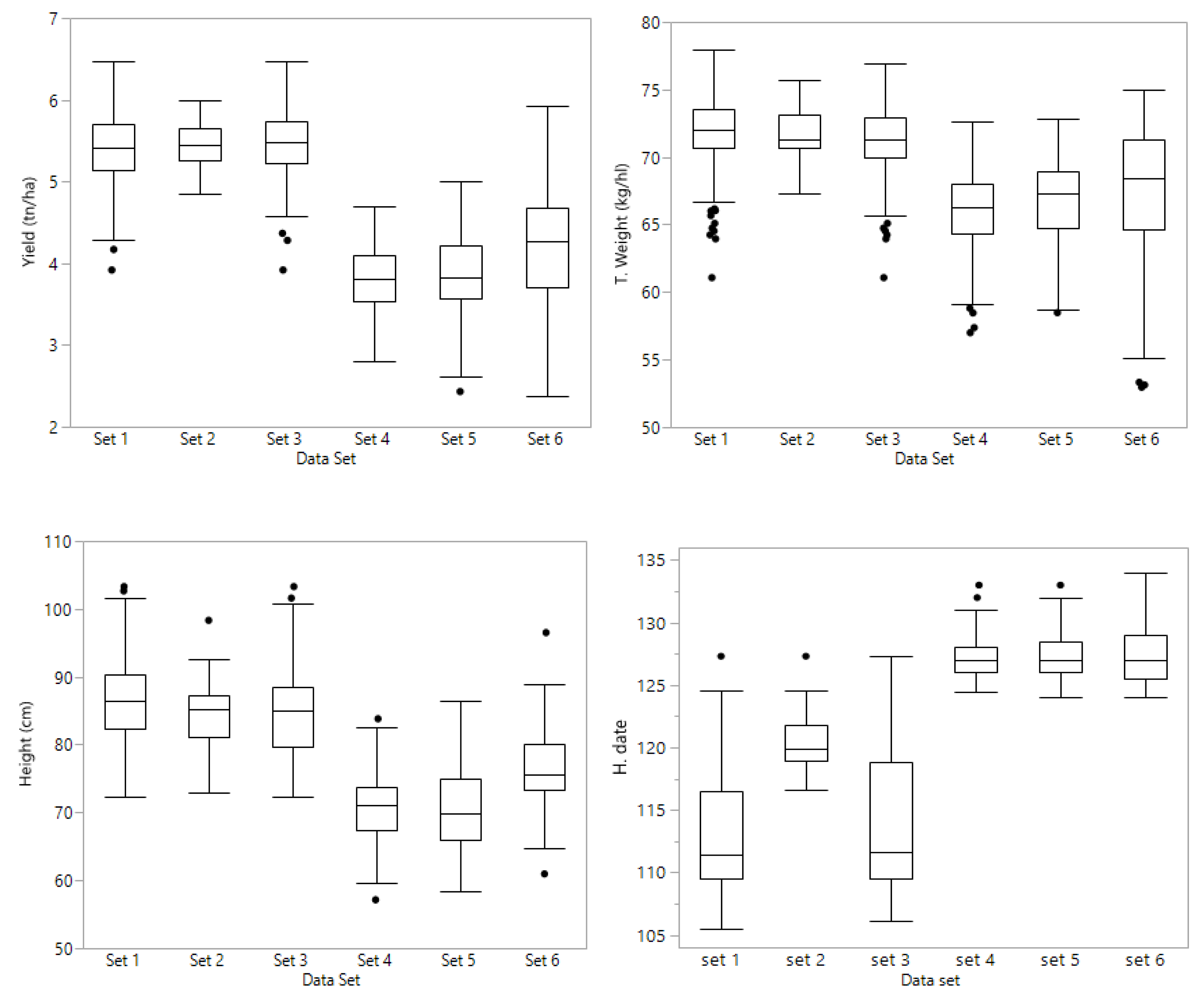
Preliminary lines were grouped by putting together families with common parents, making sure that each family has at least one half sib family in the same set. Therefore, sets 4, 5, and 6 have full sibs, half sibs, and lines with no common parents. Sets 4 and 5 comprised PYT lines that were tested in an unreplicated, augmented design at Lexington and Princeton, KY in 2018; set 6 was grown in Princeton and Midway, KY in 2018. Set 4 consisted of 141 PYT lines consisted in nine families ranging from 7 to 37 lines each. Set 5 consisted of 163 PYT lines comprising eleven families ranging from 9 to 24 lines in each family. Set 6 consisted of 146 PYT lines; there were ten families with a range of 10 to 20 lines per family. A complete chart of the data sets is shown in Figure 1.

2.2. Phenotyping

The experimental design for all replicated trials at each location and in both years was a resolvable cyclic row × column with three replications. Plots consisted of six (6) rows 19 cm apart, and a length of 4 m. The total plot area was harvested (4.6 m²) with a Wintersteiger combine to record grain yield (t ha⁻¹) and test weight (kg hl⁻¹). Heading date (days after 1 January) and height from the ground to the tip of the spike (cm) were recorded for each plot during the growing season.

The 451 lines (sets 4, 5, and 6) planted in unreplicated trials were evaluated during the 2018 season at two locations in Kentucky. Set 4 (141 lines) and set 5 (163 lines) in Lexington and Princeton, and set 6 (147 lines) in Midway and Princeton. Yield trials were planted as an augmented design, with check cultivars every five (5) plots. Two SRW cultivars, Truman (late, tall, photoperiod sensitive, excellent scab resistance) and Pembroke 2016 (early, short, photoperiod insensitive, good scab resistance) were allocated to experimental units in such a way that each group of 5 experimental lines was flanked by these two check cultivars. Experimental lines were randomly allocated to available experimental units throughout the experiment. Each range of plots was regarded as a block, and an error mean square was generated from the block x check cultivar interaction. Plots consisted of six (6) rows 19 cm apart, and a length of 4 m. The total plot area (4.6 m²) was harvested to record grain yield and test weight. Heading date and height were recorded for each plot during the growing season.

2.3. Genotyping

DNA was extracted using the sbeadex plant kit from BioSearch Technologies; using leaf samples from the F_4:5 or F_4:6 lines that were collected by sampling a minimum of eight 7–10 day old seedlings.

Genotyping by sequencing (GBS) [22] using the protocol described by Poland et al. [23] was conducted for the 816 lines that were phenotyped. Single nucleotide polymorphism (SNP) calling on raw sequence data was done with Tassel-5GBSv2 pipeline version 5.2. 35 SNPs with ≤50% missing data, ≥5% minor allele frequency and ≤10% of heterozygous calls per marker locus were retained and imputation performed using Beagle v4.0. The final number of SNPs utilized for analysis was 21,643. With the genome wide marker information, a kinship matrix including the 816 lines was built in Tassel-5GBSv2. Principal components analysis was generated with Tassel-5 and the eigenvalues for PC1 and PC2 were plotted, and there was no underlying structure identified in the population.

2.4. Genomic Prediction

GEBVs for grain yield, test weight, heading date, and height were estimated using ridge regression best linear unbiased prediction (RR-BLUP) [24] with the model

y = Xβ + Zu + e

(10)

where y is a vector of BLUEs for one trait for each wheat genotype, β is a vector of fixed effects which includes the overall mean and fixed covariates (major QTL and association mapping markers), X and Z are the design matrices for fixed and random effects, respectively, and u is a vector representing residual terms. The variance–covariance structure associated with the random term was u~N (0, Iσ_u²) and for the residual term was e~N (0, Iσ_e²). The estimates of u were obtained from the mixed.solve function using the package RR-BLUP in R [25]. Prediction accuracy was defined as the Pearson correlation between the phenotypic values (BLUEs) and the GEBVs (predicted) values.

2.5. Cross Validation

We first investigated the predictive ability of the genomic selection model for each of the four traits calculating the Pearson correlation between the phenotypic values (BLUEs) and the GEBVs (predicted) values across 100 iterations of cross validation. A random sampling cross validation scheme was conducted for all traits, in the six sets described previously. The cross validation randomly assigned 80% of the total lines to the TP and the other 20% lines to the VP.

2.6. Design of the Training Populations

To achieve the goal of this study, evaluating different schemes of applying GS at the PYT level, three different approaches to designing the training population were investigated. The first approach consisted of establishing sets 1, 2, and 3 as the TP. As described previously, these lines belong to advanced trials of the UK wheat breeding program. Sets 4, 5, and 6 with the unreplicated PYT lines were designated VP. This first strategy involved running the GS model with a TP consisting of advanced UK breeding lines phenotyped over several locations for two years. The second scheme only included sets 4, 5, and 6, the PYT lines, and consisted of building TPs such that 50% of the lines of all families within each set became the TP and were used to predict the other 50%. Within a set, each family was randomly split in half, therefore every family was represented both in the TP and VP. The third scheme consisted of a within family approach. For this approach, the same genotypes assigned to the TP or VP in the second approach described previously, were used as TP or VP, but GS was run for each family individually, obtaining a prediction accuracy for each family. Subsequently, the average prediction accuracies and standard errors were calculated for each set (4,5,6) using family means.

2.7. Selection of Best and Worst Performing Lines Based on Ranking and Different Selection Intensity

The assessment of the performance of the lines in the field (phenotypic data) and the correlation with GEBVs obtained with GS was performed in this way: for each set separately, a ranking of the lines from highest to lowest yield was made based on the field grain yield and another ranking was made based on the predicted yields obtained with GS. Different selection intensities were chosen, 10, 20, 30, and 40%. With these selection intensities we calculated for each data set the proportion of lines selected for high yield (top performers), and low yield (poorest performers) based on BLUES and GEBVs. Afterwards, we compared both selections and calculated the percentage of lines selected based on phenotypic data that would have been also selected using the GEBVs.

3. Results

3.1. Phenotypic Summary

Boxplots for grain yield, test weight, heading date, and plant height are shown in Figure 2. Average grain yield, test weight, and height were greater in sets 1, 2, and 3 than in sets 4–6, though differences were not always significant. The average yield ranged from 5.41 to 5.47 t ha⁻¹, average test weight ranged from 71.23 to 71.95 kg hL⁻¹ and average height ranged from 84.32 to 86.19 cm. On the other hand, the sets of preliminary lines (set 4, 5, 6) that were only evaluated in 2018 showed lower values for these traits. Average yield ranged from 3.8 to 4.2 t ha⁻¹, average test weight ranged from 66 to 66.7 kg hL⁻¹ and average height ranged from 70.4 to 76.4 cm. Boxplots for heading date showed earlier heading dates for sets 1, 2, and 3 compared to sets 4, 5, and 6.

3.2. Cross Validation

To evaluate the ability of the model to estimate the GEBVs for the different traits, 100 cycles of cross validation were run and prediction accuracy calculated (

Table 1. Means and standard errors of prediction accuracy of the different traits for the six wheat breeding populations with cross validation. Grain yield (t ha⁻¹), test weight (kg hL⁻¹), heading date (days after 1 January) and height (cm).

SET	Grain Yield	Test Weight	Heading Date	Height
Set 1	0.511 ± 0.01	0.712 ± 0.01	0.416 ± 0.01	0.676 ± 0.01
Set 2	0.329 ± 0.02	0.497 ± 0.02	0.444 ± 0.02	0.350 ± 0.03
Set 3	0.513 ± 0.01	0.676 ± 0.01	0.361 ± 0.01	0.708 ± 0.01
Set 4	0.361 ± 0.01	0.495 ± 0.01	0.469 ± 0.02	0.451 ± 0.01
Set 5	0.603 ± 0.01	0.683 ± 0.01	0.760 ± 0.01	0.621 ± 0.01
Set 6	0.552 ± 0.01	0.630 ± 0.01	0.698 ± 0.01	0.397 ± 0.01

). Prediction accuracies were moderate to strong for the different traits. Prediction accuracy for yield ranged from 0.33 in Set 2 to 0.60 in set 5. For test weight, prediction accuracy ranged from 0.49 in set 4 to 0.71 in set 1. Prediction accuracy of heading date ranged from 0.36 in set 3 to 0.76 in set 5, while prediction accuracy for height ranged from 0.35 in set 2 to 0.71 in set 3.

3.3. Genomic Prediction of Preliminary Lines with Advanced Lines as TP

Genomic selection has become a tool routinely used by wheat breeding programs, where breeding populations generally consist of multiple families of small size; because of this aspect it is crucial to determine the most practical and cost-effective way to apply GS to predict preliminary lines’ performance. The use of sets 1, 2, and 3 as TPs to calculate GEBVs for sets 4, 5, and 6 (VPs) (

Table 2. Prediction accuracy for wheat grain yield (t ha⁻¹), test weight (kg hL⁻¹), heading date (days after 1 January) and height (cm) using advanced line training populations to predict preliminary line performance. TP = training population; VP = validation population.

	Grain Yield				Test Weight
TP	VP			TP	VP
	Set 4	Set 5	Set 6		Set 4	Set 5	Set 6
Set 1	0.175	−0.232	0.335	Set 1	0.276	0.246	−0.119
Set 2	0.075	−0.210	0.307	Set 2	0.293	0.162	0.315
Set 3	0.060	−0.263	0.258	Set 3	0.353	0.267	0.029
	Heading Date				Height
TP	VP			TP	VP
	Set 4	Set 5	Set 6		Set 4	Set 5	Set 6
Set 1	−0.041	0.109	0.306	Set 1	0.070	0.325	0.231
Set 2	0.079	0.198	0.501	Set 2	0.103	0.171	0.046
Set 3	−0.079	0.310	0.388	Set 3	0.175	0.296	0.146

) generally showed low to moderate prediction accuracy. Prediction accuracy for grain yield ranged from −0.26 to 0.33 (set 1 predicting set 6), for test weight prediction accuracy ranged from −0.12 to 0.35 (set 3 predicting set 4). For heading date, prediction accuracies ranged from −0.08 to 0.50 (set 2 predicting set 6) and for height, prediction accuracy ranged from 0.05 to 0.32 (set 1 predicting set 5).

All predictions were low to moderate, regardless of the data set used as TP. Regarding the VP, the highest prediction accuracy for yield and heading date was found for set 6. Set 4 had the highest prediction accuracy for test weight and set 5 had the highest prediction accuracies for height (Table 2).

3.4. Genomic Prediction of 50% of Each Preliminary Line Set with the Remaining 50%

The second approach, including 50% of each family in the TP and the other 50% in the VP for each data set of preliminary lines, showed moderate to strong prediction accuracies for all traits (

Table 3. Prediction accuracy for wheat grain yield (t ha⁻¹), test weight (kg hL⁻¹), heading date (days after 1 January) and height (cm). TP = training population; VP = validation population. TP is formed by 50% of lines of each family; all families are part of TP and VP.

TP	VP	Grain Yield	Test Weight	Heading Date	Height
Set 4 (50%)	Set 4 (50%)	0.130	0.475	0.368	0.325
Set 5 (50%)	Set 5 (50%)	0.646	0.593	0.702	0.492
Set 6 (50%)	Set 6 (50%)	0.490	0.614	0.725	0.504

). For grain yield, prediction accuracy ranged from 0.13 to 0.65, for test weight prediction accuracy ranged from 0.47 to 0.61, for heading date prediction accuracy ranged from 0.37 to 0.72 and for height, prediction accuracy ranged from 0.32 to 0.50. Both sets 5 and 6 showed moderate to strong prediction accuracies for all traits. On the other hand, set 4 showed the lowest prediction accuracies ranging from 0.13 for yield to 0.47 for test weight.

3.5. Genomic Prediction Within Families for Each Set of Preliminary Lines: 50% of the Family in the TP and 50% of the Family in the VP

This third approach, where GS was applied to each family individually, showed low to moderate prediction accuracies for all traits (

Table 4. Mean prediction accuracy and standard error of the mean for wheat grain yield (t ha⁻¹), test weight (kg hL⁻¹), heading date (days after 1 January) and height (cm). Genomic selection was applied to each family individually. Values of prediction accuracy are the average accuracies among families for each data set.

SET	Grain Yield	Test Weight	Heading Date	Height
Set 4	−0.036 ± 0.25	0.385 ± 0.13	−0.159 ± 0.15	0.058 ± 0.14
Set 5	0.231 ± 0.07	0.363 ± 0.16	0.301 ± 0.16	−0.129 ± 0.14
Set 6	0.335 ± 0.12	0.167 ± 0.15	0.390 ± 0.15	−0.085 ± 0.12

). For grain yield, prediction accuracy ranged from −0.036 to 0.33, for test weight, prediction accuracy ranged from 0.17 to 0.38, for heading date prediction accuracy ranged from −0.16 to 0.39 and for height prediction accuracy ranged from −0.13 to 0.05. Only test weight presented average positive prediction accuracies for all sets. Set 5 and 6 had prediction accuracies low to moderate for three out of four traits.

3.6. Impact of Different Prediction Accuracies on the Identification of Best and Worst Performing Lines

Prediction accuracy for grain yield was 0.13 in set 4, 0.65 in set 5, and 0.49 in set 6 (Table 3) and these values could have serious implications for the big question a breeder has to answer: how many lines for a given trait were correctly selected with the GS model?

Table 5. Percentage of correctly selected highest and lowest yielding wheat breeding lines at different selection intensities (10–40%), for the different data sets. Prediction accuracy for yield when 50% of each set predicted the other 50% was set 4 = 0.13, set 5 = 0.65 and set 6 = 0.49.

			Selection Intensity
		10%	20%	30%	40%
Highest Yielding Lines	set 4	0	7	19	36
	set 5	50	75	79	75
	set 6	28	57	57	68
Lowest Yielding Lines	set 4	0	36	57	53
	set 5	25	50	46	62
	set 6	28	36	48	61

shows the percentage of lines chosen correctly based on the GEBVs for grain yield at different selection intensities, when selecting the best yielding lines or identifying the worst yielding lines.

In terms of identifying the best yielding lines, a prediction accuracy of 0.65 (set 5) meant a 75–79% of lines were selected correctly when selection intensity was between 20–40%; at a higher selection intensity, for example 10%, only 50% of lines were correctly selected. With a prediction accuracy of 0.49 (set 6) a 57–68% of lines were selected correctly when selection intensity was between 20–40% while only 28% of lines were selected correctly at a selection intensity of 10%. Finally, with a prediction accuracy of 0.13 (set 4) between 19–36% or the lines were correctly selected in a selection intensity between 30–40%. With a 10% selection intensity, none of the best performing lines were correctly selected (Table 5).

To identify the worst performing lines, for the three sets, the proportion of correctly selected lines was between 36–50% when selection intensity was 20%, between 46–57% of the lines were identified correctly when selection intensity was 30% and the proportion of correctly selected lines was between 53–62% with a selection intensity of 40%. At the highest selection intensity, 10%, set 4 had almost zero correctly selected lines and both set 5 and 6 had a total of 35% lines correctly selected as the poorest performers.

For set 4, the set with lowest prediction accuracy for grain yield (0.13), the identification of the worst performing lines was more successful than the identification of the top yielding lines.

3.7. Analysis of Kinship Based on Within-Family Genetic Relationships

First, based on the genomic relationship matrix (GRM), a principal components analysis (PCA) was done and did not reveal any underlying structure in the data. Next, we calculated the kinship for each family and calculated a kinship family mean for each data set. Figure 3 summarizes kinship for each set. Average kinship was 0.60 for set 4, 0.82 for set 5, and 1.01 for set 6. Kinship varied for set 4 from 0.24 to 0.88; for set 5 from 0.25 to 2, and for set 6 kinship varied from 0.54 to 1.29.

3.8. Effect of Phenotypic Variation Based on Family Means for Grain Yield

With the objective to investigate the differences in prediction accuracy for yield between the three data sets, we analyzed the phenotypic expression for this trait among families within each data set. Average yield based on family means (Figure 4) was 3.79 t/ha for set 4 with a range of 3.61–3.97; set 4 showed the lowest variation between families for this trait. Average yield among families in set 5 was 3.84 t/ha showing a higher range of 3.56–4.38 t/ha. Average yield in set 6 was the highest, 4.16 t/ha, with the largest variation between families ranging from 3.37 to 4.85 t/ha.

4. Discussion

Applying GS in plant breeding has become a primary technology for breeders looking for strategies to accelerate the breeding process. Some of the benefits of GS pursued by breeders when estimating GEBVs in their breeding programs include increasing genetic gain per unit time, reduced phenotyping costs, reducing field testing in early stages, and more accurate selection of parents for crosses.

Commercial and public breeding programs, mainly in small grains, have some differences that make them unique and affect the optimal stage of applying genomic selection. Many questions arise concerning the design of the TP, including size of the TP and the relatedness between TP and VP. Also of great concern is the usefulness of GS at different stages of the breeding program and how to allocate the resources, at the field testing level, where preliminary trials become a key stage because of the limited amount of seed for field plots and the high number of untested lines the breeder must evaluate.

Therefore, the goal of this study was to evaluate different schemes to apply GS at the PYT level in the hope of drawing inferences about the different strategies that could help breeders when implementing GS. Overall, results from our study were encouraging regarding the prediction of preliminary lines, even for highly polygenic and complex traits like yield and test weight. The model’s predictive ability, with cross validation, showed moderate to high accuracies for the different traits, in agreement with previous studies on wheat [11,13,15,26,27,28].

Prediction accuracy for yield ranged from 0.33 to 0.6 for the six data sets. Different authors have reported similar or lower prediction accuracies for grain yield; Heffner et al. [26] using different models under a cross validation scheme reported prediction accuracies of around 0.2. Isidro et al. [13] applying different strategies to define the TP, obtained for wheat populations with a mild population structure, prediction accuracies ranging from 0.2–0.5, noting an increase of prediction accuracy with increases in TP size. Recently, Sarinelli et al. [15] obtained prediction accuracies ranging from 0.4 to 0.6 under different methods of selecting the TP and different TP sizes.

The other traits under study—test weight, heading date, and height—showed moderate to strong prediction accuracies in each of the different sets. In general, we obtained higher accuracies compared to yield, as one would expect for heading date and height, because of the genetic architecture of these traits based on fewer QTLs than yield. On the other hand, for test weight which is also a complex polygenic trait under a high environmental influence, we obtained higher prediction accuracies than some previous studies [13,15,27].

4.1. Applying GS at the PYT Level

A frequent question for breeders is which is the best strategy to predict the performance of untested lines, and how to allocate resources to exploit the maximum genetic diversity for each breeding population that reaches the testing stage, despite the need to allocate many resources to the testing of lines in replicated trials over different environments. The different strategies of designing the TP that we applied could be used routinely by breeders. The first of these was to use advanced lines of the same breeding program as the training population (Table 2). This strategy has the advantage of having lines in the TP phenotyped at more than a single environment, which has shown a positive effect on prediction accuracy [5,29].

As a pitfall, sets including advanced lines generally are constituted by many families, with a small number of lines per family, which can reduce linkage disequilibrium between markers and QTLs when running the model. Additionally, close relatives share long haplotypes and this leads to advantages for genomic predictions [10], but these can be lost or reduced when advancing only a few lines per family. Predicting preliminary lines with advanced material has been investigated by Michel et al. [11], who reported prediction accuracies of 0.39 for yield and 0.5 for protein content. They reported higher accuracies for yield, reaching 0.48, when they estimated GEBVs for tested preliminary lines in untested years, adding data of the preliminary lines to the model.

In our study, predicting untested lines with advanced lines from the wheat breeding program (set 1, 2 3), showed low prediction accuracies for set 4 and 5, and better prediction accuracies ranging from 0.25–0.33 in set 6. For yield, the biggest training population, set 1 (361 lines) showed better prediction accuracies both for set 4 and 6 higher than smaller TPs like sets 2 and 3. Even though set 2 was formed by the selected lines of the breeding program, with two years of multi-environment, balanced data it was not successful as a TP for different sets of preliminary lines. Set 2 showed also the lowest prediction accuracy with cycles of cross validation for all traits. These results do not agree with Tiede et al. [30], who showed in a barley study that a TP to which selected lines had been added had an overall positive effect on prediction accuracy. In our study, set 1 (361 lines) and set 3 (226 lines) showed for all traits more consistent results than set 2 (70 lines). We conclude that at small TP size like set 2, the relatedness between TP and VP is a critical issue and despite inclusion of selected genotypes from the breeding program, the TP formed by a few lines of multiple families with variable degrees of relatedness does not give consistent and accurate results. This is in agreement with Hickey et al. [10], who show similar results in a simulation study in maize.

4.2. Relationship between TP Size and Relatedness among and within Families

Not much information is found in the literature regarding the use of small training populations when predicting preliminary lines. The next scheme we investigated was the use of preliminary lines themselves as the training populations, splitting each set in half where 50% of the lines become the TP to predict the other half that becomes the VP (Table 3).

We obtained moderate to strong prediction accuracies (0.5–0.7) for all traits in sets 2 and 3 (Table 3), obtaining values similar to the ones obtained with cross validation (Table 1) showing the success of this approach. In a simulation study, with a TP containing genotypes half sibs and grandparents to the selection candidates, Hickey et al. [10] reached prediction accuracies of 0.4 with TP size of 260 genotypes. They obtained prediction accuracies of 0.6 when increasing the number of lines per family from 5 to 50, with the consequent increase in total TP size (600–2600 genotypes). Our results are very encouraging as we obtained prediction accuracies ranging from 0.5–0.7 with TP sizes of 70–85 genotypes.

When GS was applied within families, which meant including only full sibs in TP and VP (Table 4), we observed inconsistent results with high levels of variation among families, and low prediction accuracies. In this study we worked with families that had from 8 to 25 individuals each, which is a common population size in wheat. This approach brings up the discussion of the appropriate family size to apply GS to predict full sib performance. Within families, cross validation shows variable prediction accuracies at small TP sizes [16,27], in agreement with our results (data not shown). Hickey et al., [10] suggested that families with more than 50 individuals are needed for a within family cross validation to obtain accuracies of 0.4 or more. Despite the fact that our selection strategy illustrated in Table 4 is different from cross validation, we agree that larger families than the ones we had are more likely give more consistent results. Furthermore, with our approach of splitting the family 50:50 among TP and VP, a TP of more than 50 genotypes might assure better predictions, though more research should be done to investigate this approach. Our results strongly support that pooling together a group of families, therefore, having full sibs, half sibs, and more distant material in the TP and VP, is essential when using small TPs, rather than having only full sibs, given the size of each family (8–25 lines). Smaller families create the need to pay extra attention to the relatedness within and among families.

We also investigated whether levels of kinship based on genome wide markers (GWM) could account for the differences in prediction accuracy for the different data sets of preliminary lines. The average kinship, based on family means, for each set (Figure 4) showed that sets 5 and 6, in which we obtained better predictive values, had on average, higher mean family kinship compared to set 4, the set with lower prediction accuracies. These results do not agree with those found by Marulanda et al. [31] who found that levels of kinship were not associated with the prediction accuracy, at smaller TP sizes. More research should be done to confirm whether a breeder working with small sets of lines could establish a TP with diverse number of families based on GWM information, or if pedigree information is better for making decisions on the TP regarding relatedness between families.

4.3. Meaning of Different Prediction Accuracies from a Breeder’s Standpoint

The research on GS has increased tremendously in the last few years, where many studies approach the question about how well a training model can generate accurate GEBVs. The success of GS is always evaluated through the prediction accuracy, the Pearson correlation between the GEBVs and the actual phenotypic values, typically BLUEs like least squares means. Prediction accuracy overall does a good job in evaluating the predictive ability of a model, assessing the value of different training populations, or different optimization methodologies of the training populations. Yet what are the implications for actual breeding programs, of a 0.3 vs. a 0.7 prediction accuracy? This issue is discussed by Bassi et al. [2] asking the question: “how many of the top 5% individuals for a given trait are correctly selected at different levels of prediction accuracy”.

Our goal was to get a better understanding of this question, and these results provide some insights about the outcomes a breeder may expect when establishing a GS scheme in their breeding program. Table 3 showed encouraging results predicting different traits. For grain yield, a complex trait which is generally the first breeding target in almost all breeding programs, the three sets showed prediction accuracies ranging from 0.13 to 0.65. Using these results, we analyzed the proportion of correctly selected lines at different selection intensities (Table 5). Our results confirm the suggestion of Bassi et al. [2] and Table 5 showed that with a selection intensity of 20%, usually common for breeders when selecting at early stages of testing and with a prediction accuracy of 0.49 (set 6) the 57% of the top performers were correctly selected with GS, greater than the expected 49% given by the Pearson’s correlation. With the same selection intensity and with a prediction accuracy of 0.65 (set 5) 75% of the highest yielding lines were correctly selected by this model. If we looked at the possibility of discarding the poorest performing lines, the proportion of correctly discarded lines is lower, with a 20% of selection intensity, up to a 50% of the lines are correctly discarded, but surprisingly even with a prediction accuracy of 0.13 (set 4), at 20% selection intensity around a 40% of the poorest performing lines were selected correctly. The caveat here is that the best performing lines are not necessarily the lines with the highest true breeding values, but are rather the highest performing based on phenotypic results from unreplicated yield trials at two locations in one year.

These results try to walk over the bridge between the academic results and the actual breeding program’s needs, and offer encouragement to breeders in terms of applying GS in their breeding programs. Even for polygenic, complex traits like yield, prediction accuracies of more than 0.4 could bring about successful results, when using a selection intensity of 20%. In scenarios where the breeder applied a lower selection intensity (30%), 57% and 79% of the top performers were selected with prediction accuracies of 0.49 and 0.65 respectively (Table 5).

We can conclude that the model had a better ability to predict the extreme values, estimating accurate GEBVs for the top performers and in second place the poorest performers, but it was not so successful in estimating the average performers. Our results do not agree with Ornella et al. [32] who suggested that Pearson correlation coefficient may not be the appropriate measure because it does not evaluate the quality of the regression at the tails of the distribution; our results suggest that it does a good job assessing and estimating the individuals at the top of the rank, and does a poor job in predicting the average performers, or finding the top individuals when selection intensity is 10%. Ornella et al. [32] proposed the use of classification algorithms that construct a decision boundary that separates two classes, best lines and worst lines, as a promising alternative approach to regression methods for GS, and we think that this issue should receive more attention considering the implications of the use of prediction accuracy. So far, with these results, we suggest that a prediction accuracy of 0.5 should be considered very valuable when predicting for complex traits like yield, at a selection intensity of 20%.

4.4. Practical Implementation of GS and the Question of Redesigning a Wheat Breeding Program

Our study showed some strategies that may be followed by breeders when trying to predict PYT lines with GS, always focusing on predicting untested lines. Our data prompts us to suggest that an efficient and successful approach for a breeder with limited resources, as an alternative to developing extensive training populations that increase phenotyping costs, is to test half of the genotyped PYT lines and use those lines to predict performance of the other half of the preliminary lines. Pooling together families with different levels of relatedness but always including full sibs and half sibs, will ensure there are related lines in the TP and VP, a recommended strategy when designing small training populations of early generation material.

How can we be confident we will not have a set of lines, that will give prediction accuracies of 0.13 for yield, as we have for set 4 (Table 3), knowing that many factors interact and influence the prediction accuracy? There is no correct answer, but some decisions the breeder can make will reduce the likelihood of this outcome. Previous studies showed low prediction accuracies when the TP had fewer than 50–75 individuals [10,13,28,33]. Additionally, small TPs increase the dependence on the phenotypic variance [31]. We worked with TP size around 70–80 lines for this strategy (Table 3), and the effect of a low phenotypic variance for yield in set 4 (Figure 4) could be seen in our results when looking at prediction accuracy for grain yield in that set. In a TP simulation study, Hickey et al. [10] showed that with eight families, half sibs to the VP, with 50 lines each family (TP = 400 genotypes), they reached a prediction accuracy of 0.6 at different SNP densities. We worked with sets with 8–10 families each, but as noted, our family size was 8–25 individuals, much lower than that used in the simulation study as well as other studies working with breeding populations [8,9,34].

Our work leads us to conclude that a minimum of 25 lines per family is needed to stabilize the prediction accuracies, therefore pooling together 8–10 families the breeder would have a total of 200–250 lines to split among TP and VP. Under this scheme, only lines in the TP will be phenotyped during the field season. In order to ensure there would be seed for testing the selection candidates the following year, the lines in the VP could be planted in plots, or even in several head rows, to reduce costs and area used for field testing. After harvesting the lines in the TP, the GEBVs for yield and other traits will be predicted on the VP and the selection candidates will be harvested based on the GEBVs, and other information the breeder considers useful.

Finally, larger families at the preliminary yield trial level generally implies in most breeding programs an increase in the size of segregating populations developed by the breeder. So here the question about resource allocation arises, and whether bigger segregating populations should be made to the detriment of the number of populations created. Related to this topic, Bernardo et al. [33] concluded that large selection responses could be achieved with a wide range of combinations between number and size of breeding populations and that again, the issue of parental selection is more important than the issue of number versus size of breeding populations. Witcombe et al. [35] with a simulation study also suggests that the probability of success in a breeding program could be achieved with fewer crosses more carefully chosen and bigger segregating populations. This topic has recently been discussed by Gorjanc et al. [36], when they simulated the results of applying an optimal cross selection scheme to balance selection and maintenance of genetic diversity for breeding programs under a recurrent genomic selection scheme. They showed the benefits of the optimal cross selection, and the positive implications for maintaining genetic diversity and genomic prediction accuracy in the long term.

Therefore, increasing the size of segregating populations with a reduction in the total number of populations evaluated may be a valid alternative to achieve larger family size at the PYT stage. Accompanying this would be an increased focus on selecting parents for crosses using, for example, the R package POPVAR [37] or other methods.