
Molecular Simulation of the Isotropic-to-Nematic Transition of Rod-like Polymers in Bulk and Under Confinement


Abstract

1. Introduction
2. Methodology
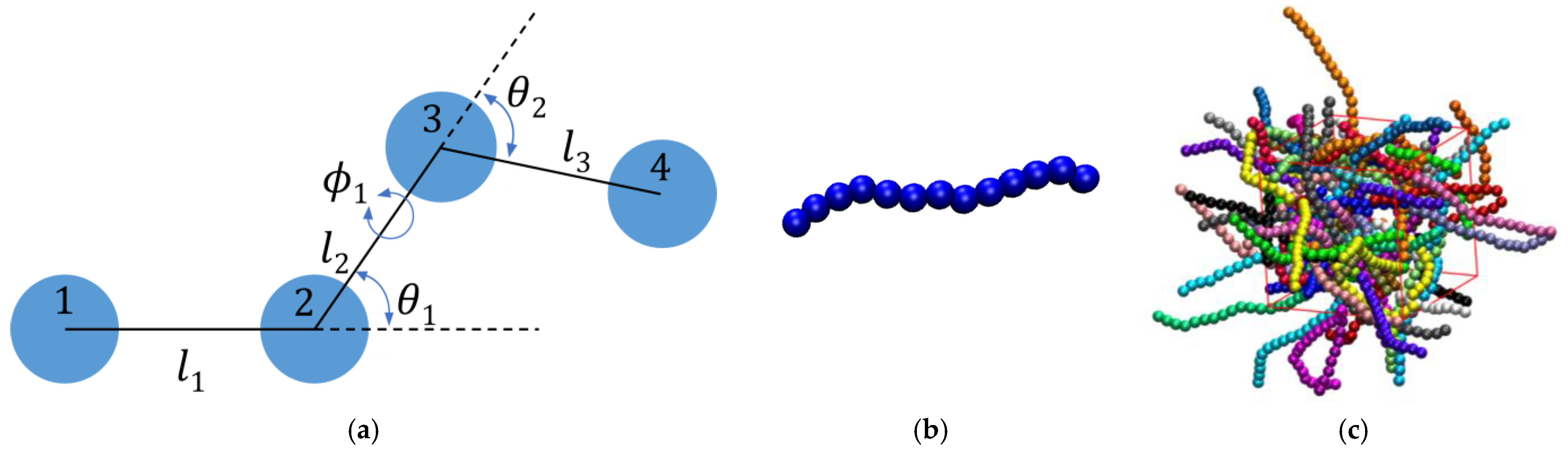
2.1. Molecular Model
2.2. Simulation Algorithm
2.3. Long-Range Order
3. Results
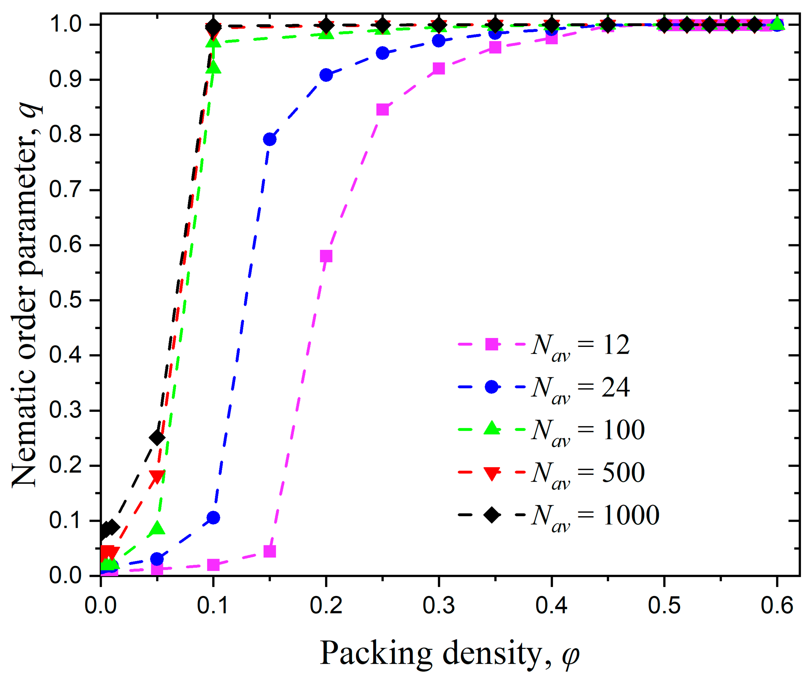
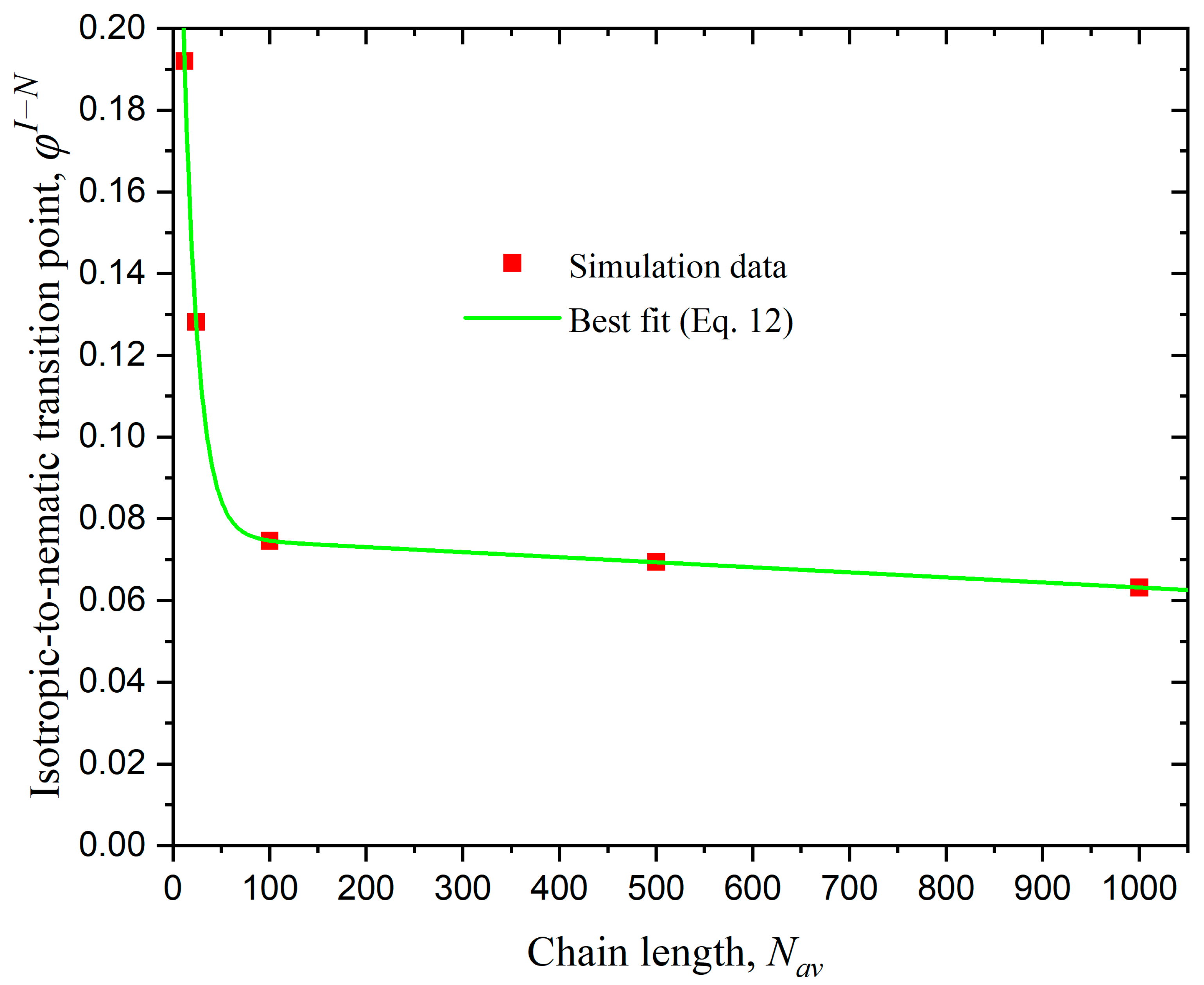
3.1. Effect of Chain Length
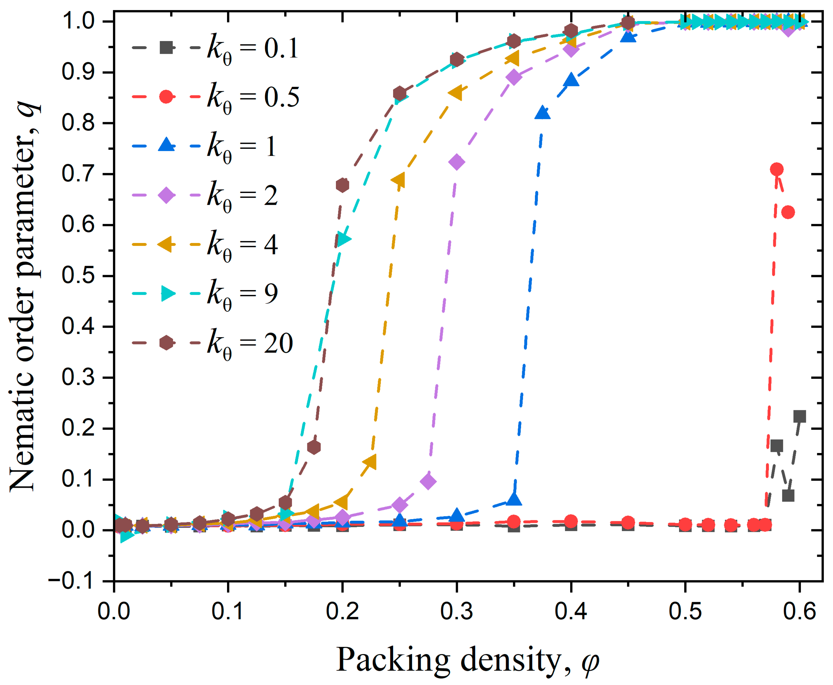
3.2. Effect of Chain Stiffness
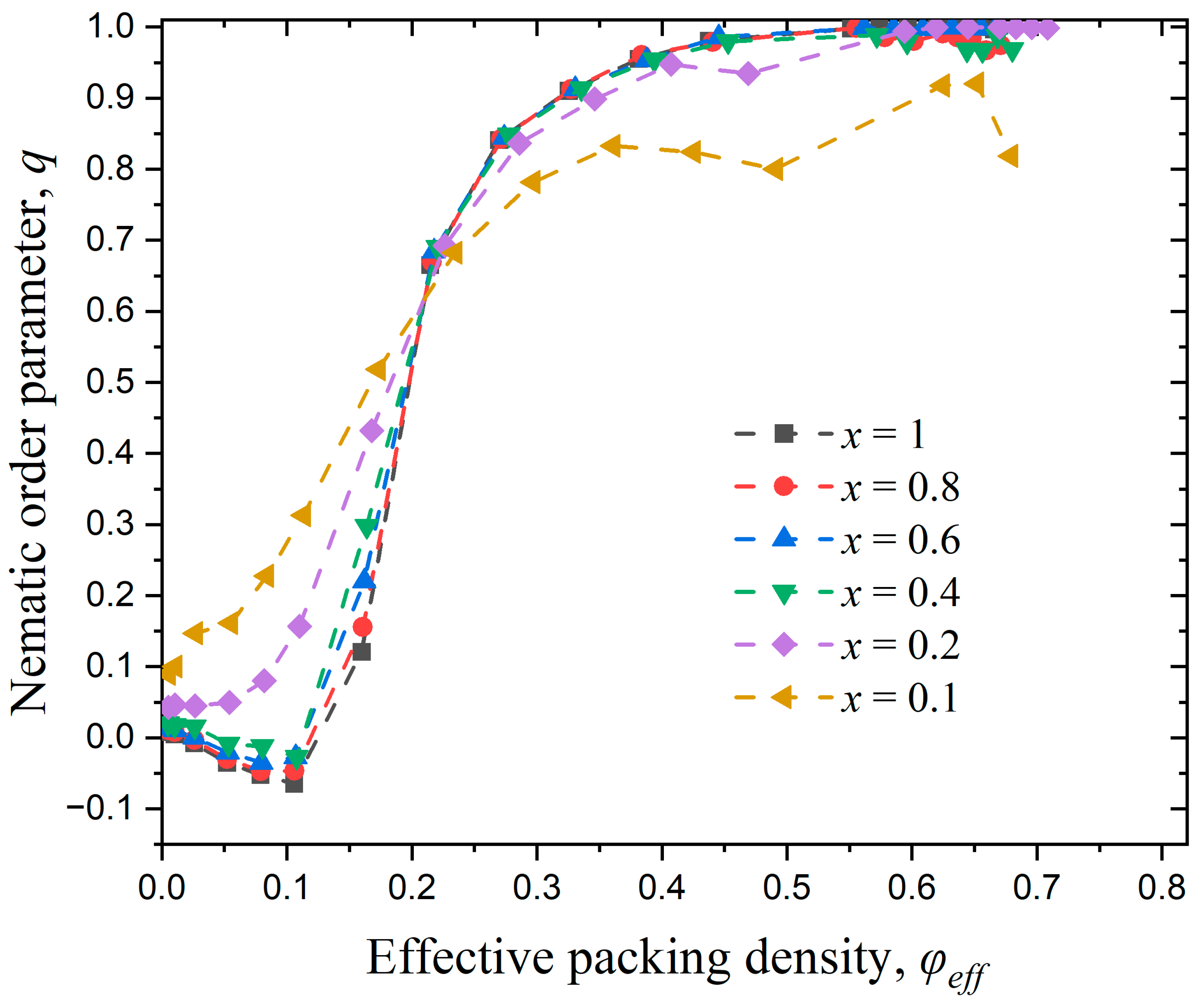
3.3. Effect of Confinement
3.3.1. Effect of Confinement in One Dimension
3.3.2. Effect of Confinement in Two Dimensions
3.3.3. Effect of Confinement in Three Dimensions
4. Conclusions
Author Contributions
Funding
Institutional Review Board Statement
Data Availability Statement
Acknowledgments
Conflicts of Interest
References
- Flory, P.J. Principles of Polymer Chemistry; Cornell University Press: Ithaca, NY, USA, 1953. [Google Scholar]
- Flory, P.J. Statistical Mechanics of Chain Molecules; Hanser-Verlag: Munchen, Germany, 1989. [Google Scholar]
- deGennes, P.G. Scaling Concepts in Polymer Physics; Cornell University Press: Ithaca, NY, USA, 1980. [Google Scholar]
- Doi, M.; Edwards, S.F. The Theory of Polymer Dynamics; Clarendon Press: Oxford, UK, 1988. [Google Scholar]
- Likhtman, A.E.; McLeish, T.C.B. Quantitative theory for linear dynamics of linear entangled polymers. Macromolecules 2002, 35, 6332–6343. [Google Scholar] [CrossRef]
- Lee, W.; Shih, Y.-C. Effects of carbon-nanotube doping on the performance of a TN-LCD. J. Soc. Inf. Disp. 2005, 13, 743–747. [Google Scholar] [CrossRef]
- Seo, D.-S.; Han, J.-M. Generation of pretilt angle in NLCs and EO characteristics of a photo-aligned TN-LCD with oblique non-polarized UV light irradiation on a polyimide surface. Liq. Cryst. 1999, 26, 959–964. [Google Scholar] [CrossRef]
- Shunsuke, K.; Yasufumi, I. Multidomain TN-LCD fabricated by photoalignment. In Proceedings of the Conference on Liquid Crystal Materials, Devices and Applications V, San Jose, CA, USA, 12–13 February 1997; pp. 40–51. [Google Scholar]
- Lien, C.-H.; Guu, Y.H. Optimization of the Polishing Parameters for the Glass Substrate of STN-LCD. Mater. Manuf. Process. 2008, 23, 838–843. [Google Scholar] [CrossRef]
- Katayama, M. TFT-LCD technology. Thin Solid Film. 1999, 341, 140–147. [Google Scholar] [CrossRef]
- Fan, S.-K.S.; Chuang, Y.-C. Automatic detection of Mura defect in TFT-LCD based on regression diagnostics. Pattern Recog. Lett. 2010, 31, 2397–2404. [Google Scholar] [CrossRef]
- Uchikoga, S.; Ibaraki, N. Low temperature poly-Si TFT-LCD by excimer laser anneal. Thin Solid Film. 2001, 383, 19–24. [Google Scholar] [CrossRef]
- Donald, A.M.; Windle, A.H.; Hanna, S. Liquid Crystalline Polymers; Cambridge University Press: Cambridge, UK, 2006. [Google Scholar]
- de Gennes, P.G.; Prost, J. The Physics of Liquid Crystals, 2nd ed.; Oxford University Press: Oxford, UK, 1993. [Google Scholar]
- Ciferri, A. Liquid Crystallinity in Polymers; VCH Publishers: Weinheim, Germany, 1991. [Google Scholar]
- Meyer, R.B.; Ciferri, A.; Krigbaum, W.R. Polymer Liquid Crystals; Academic Press Incorporated: New York, NY, USA, 1982. [Google Scholar]
- Onsager, L. The Effects of Shape on the Interaction of Colloidal Particles. Ann. N. Y. Acad. Sci. 1949, 51, 627–659. [Google Scholar] [CrossRef]
- Bolhuis, P.; Frenkel, D. Tracing the phase boundaries of hard spherocylinders. J. Chem. Phys. 1997, 106, 666–687. [Google Scholar] [CrossRef]
- Khokhlov, A.R.; Semenov, A.N. On the theory of liquid-crystalline ordering of polymer chains with limited flexibility. J. Stat. Phys. 1985, 38, 161–182. [Google Scholar] [CrossRef]
- Khokhlov, A.R.; Semenov, A.N. Liquid-crystalline ordering in the solution of partially flexible macromolecules. Phys. A 1982, 112, 605–614. [Google Scholar] [CrossRef]
- Khokhlov, A.R.; Semenov, A.N. Liquid-crystalline ordering in the solution of long persistent chains. Phys. A 1981, 108, 546–556. [Google Scholar] [CrossRef]
- Yethiraj, A.; Fynewever, H. Isotropic to nematic transition in semiflexible polymer melts. Mol. Phys. 1998, 93, 693–701. [Google Scholar] [CrossRef]
- Fynewever, H.; Yethiraj, A. Phase behavior of semiflexible tangent hard sphere chains. J. Chem. Phys. 1998, 108, 1636–1644. [Google Scholar] [CrossRef]
- Allen, M.P.; Tildesley, D.J. Computer Simulation of Liquids; Oxford University Press: New York, NY, USA, 1987. [Google Scholar]
- Frenkel, D.; Smit, B. Understanding Molecular Simulation: From Algorithms to Applications, 2nd ed.; Academic Press: San Diego, CA, USA, 2002. [Google Scholar]
- Landau, D.P.; Binder, K. A Guide to Monte Carlo Simulations in Statistical Physics, 4th ed.; Cambridge University Press: Cambridge, UK, 2014. [Google Scholar]
- Rapaport, D.C. The Art of Molecular Dynamics Simulation, 2nd ed.; Cambridge University Press: Cambridge, UK, 2004. [Google Scholar]
- Paquet, E.; Viktor, H.L. Molecular Dynamics, Monte Carlo Simulations, and Langevin Dynamics: A Computational Review. BioMed Res. Int. 2015, 2015, 183918. [Google Scholar] [CrossRef]
- Soltani, M.; Raahemifar, K.; Nokhosteen, A.; Kashkooli, F.M.; Zoudani, E.L. Numerical Methods in Studies of Liquid Crystal Elastomers. Polymers 2021, 13, 1650. [Google Scholar] [CrossRef] [PubMed]
- Kroger, M. Simple models for complex nonequilibrium fluids. Phys. Rep.-Rev. Sect. Phys. Lett. 2004, 390, 453–551. [Google Scholar] [CrossRef]
- Andrienko, D. Introduction to liquid crystals. J. Mol. Liq. 2018, 267, 520–541. [Google Scholar] [CrossRef]
- Ramos, P.M.; Herranz, M.; Foteinopoulou, K.; Karayiannis, N.C.; Laso, M. Identification of Local Structure in 2-D and 3-D Atomic Systems through Crystallographic Analysis. Crystals 2020, 10, 1008. [Google Scholar] [CrossRef]
- Herranz, M.; Martínez-Fernández, D.; Ramos, P.M.; Foteinopoulou, K.; Karayiannis, N.C.; Laso, M. Simu-D: A Simulator-Descriptor Suite for Polymer-Based Systems under Extreme Conditions. Int. J. Mol. Sci. 2021, 22, 12464. [Google Scholar] [CrossRef]
- Martínez-Fernández, D.; Herranz, M.; Foteinopoulou, K.; Karayiannis, N.C.; Laso, M. Local and Global Order in Dense Packings of Semi-Flexible Polymers of Hard Spheres. Polymers 2023, 15, 551. [Google Scholar] [CrossRef]
- Frenkel, D.; Lekkerkerker, H.N.W.; Stroobants, A. Thermodynamic Stability of a Smectic Phase in a System of Hard-Rods. Nature 1988, 332, 822–823. [Google Scholar] [CrossRef]
- Stroobants, A.; Lekkerkerker, H.N.W.; Frenkel, D. Evidence for One-Dimensional, Two-Dimensional, and 3-Dimensional Order in a System of Hard Parallel Spherocylinders. Phys. Rev. A 1987, 36, 2929–2945. [Google Scholar] [CrossRef] [PubMed]
- Frenkel, D.; Eppenga, R. Evidence for algebraic orientational order in a 2-dimensional hard-core nematic. Phys. Rev. A 1985, 31, 1776–1787. [Google Scholar] [CrossRef] [PubMed]
- Doi, M. Soft Matter Physics; Oxford University Press: New York, NY, USA, 2017. [Google Scholar]
- Kroger, M. Efficient hybrid algorithm for the dynamic creation of wormlike chains in solutions, brushes, melts and glasses. Comput. Phys. Commun. 2019, 241, 178–179. [Google Scholar] [CrossRef]
- Weismantel, O.; Galata, A.A.; Sadeghi, M.; Kroger, A.; Kroger, M. Efficient generation of self-avoiding, semiflexible rotational isomeric chain ensembles in bulk, in confined geometries, and on surfaces. Comput. Phys. Commun. 2022, 270, 108176. [Google Scholar] [CrossRef]
- Milchev, A.; Egorov, S.A.; Midya, J.; Binder, K.; Nikoubashman, A. Blends of Semiflexible Polymers: Interplay of Nematic Order and Phase Separation. Polymers 2021, 13, 2270. [Google Scholar] [CrossRef]
- Milchev, A.; Binder, K. Cylindrical confinement of solutions containing semiflexible macromolecules: Surface-induced nematic order versus phase separation. Soft Matter 2021, 17, 3443–3454. [Google Scholar] [CrossRef]
- Egorov, S.A.; Milchev, A.; Nikoubashman, A.; Binder, K. Phase Separation and Nematic Order in Lyotropic Solutions: Two Types of Polymers with Different Stiffnesses in a Common Solvent. J. Phys. Chem. B 2021, 125, 956–969. [Google Scholar] [CrossRef]
- Milchev, A.; Nikoubashman, A.; Binder, K. The smectic phase in semiflexible polymer materials: A large scale molecular dynamics study. Comput. Mater. Sci. 2019, 166, 230–239. [Google Scholar] [CrossRef]
- Milchev, A.; Egorov, S.A.; Binder, K.; Nikoubashman, A. Nematic order in solutions of semiflexible polymers: Hairpins, elastic constants, and the nematic-smectic transition. J. Chem. Phys. 2018, 149, 174909. [Google Scholar] [CrossRef] [PubMed]
- Egorov, S.A.; Milchev, A.; Virnau, P.; Binder, K. A new insight into the isotropic-nematic phase transition in lyotropic solutions of semiflexible polymers: Density-functional theory tested by molecular dynamics. Soft Matter 2016, 12, 4944–4959. [Google Scholar] [CrossRef]
- Egorov, S.A.; Milchev, A.; Virnau, P.; Binder, K. Semiflexible polymers under good solvent conditions interacting with repulsive walls. J. Chem. Phys. 2016, 144, 174902. [Google Scholar] [CrossRef]
- Egorov, S.A.; Milchev, A.; Binder, K. Anomalous Fluctuations of Nematic Order in Solutions of Semiflexible Polymers. Phys. Rev. Lett. 2016, 116, 187801. [Google Scholar] [CrossRef]
- Egorov, S.A.; Milchev, A.; Binder, K. Semiflexible Polymers in the Bulk and Confined by Planar Walls. Polymers 2016, 8, 296. [Google Scholar] [CrossRef]
- Nguyen, H.T.; Hoy, R.S. Effect of chain stiffness and temperature on the dynamics and microstructure of crystallizable bead-spring polymer melts. Phys. Rev. E 2016, 94, 052502. [Google Scholar] [CrossRef] [PubMed]
- Nguyen, H.T.; Smith, T.B.; Hoy, R.S.; Karayiannis, N.C. Effect of chain stiffness on the competition between crystallization and glass-formation in model unentangled polymers. J. Chem. Phys. 2015, 143, 144901. [Google Scholar] [CrossRef] [PubMed]
- Martínez-Fernández, D.; Pedrosa, C.; Herranz, M.; Foteinopoulou, K.; Karayiannis, N.C.; Laso, M. Random close packing of semi-flexible polymers in two dimensions: Emergence of local and global order. J. Chem. Phys. 2024, 161, 034902. [Google Scholar] [CrossRef]
- Williams, M.J.; Gray, M.C. Microcanonical Analysis of Semiflexible Homopolymers with Variable-Width Bending Potential. Polymers 2025, 17, 906. [Google Scholar] [CrossRef]
- Herard, N.; Annapooranan, R.; Henry, T.; Kröger, M.; Cai, S.Q.; Boechler, N.; Sliozberg, Y. Modeling nematic phase main-chain liquid crystal elastomer synthesis, mechanics, and thermal actuation via coarse-grained molecular dynamics. Soft Matter 2024, 20, 9219–9231. [Google Scholar] [CrossRef]
- Kröger, M.; Luap, C.; Ilg, P. Ultra-slow self-similar coarsening of physical fibrillar gels formed by semiflexible polymers. Soft Matter 2025, 23, 2803–2825. [Google Scholar] [CrossRef] [PubMed]
- Luo, C.F.; Kroger, M.; Sommer, J.U. Entanglements and Crystallization of Concentrated Polymer Solutions: Molecular Dynamics Simulations. Macromolecules 2016, 49, 9017–9025. [Google Scholar] [CrossRef]
- Pedrosa, C.; Martínez-Fernández, D.; Herranz, M.; Foteinopoulou, K.; Karayiannis, N.C.; Laso, M. Densest packing of flexible polymers in 2D films. J. Chem. Phys. 2023, 158, 7. [Google Scholar] [CrossRef]
- Rogozhin, V.B.; Polushin, S.G.; Lezova, A.A.; Polushina, G.E.; Polushin, A.S. Simulation of Structural Transition in an Isotropic Melt of Nematic and Smectic Polymers. Wseas Trans. Syst. 2024, 23, 105–112. [Google Scholar] [CrossRef]
- Zhang, W.; Zou, L. Molecular Dynamics Simulations of Crystal Nucleation near Interfaces in Incompatible Polymer Blends. Polymers 2021, 13, 347. [Google Scholar] [CrossRef] [PubMed]
- Dietz, J.D.; Hoy, R.S. Two-stage athermal solidification of semiflexible polymers and fibers. Soft Matter 2020, 16, 6206–6217. [Google Scholar] [CrossRef]
- Roy, S.; Chen, Y.L. Rich phase transitions in strongly confined polymer-nanoparticle mixtures: Nematic ordering, crystallization, and liquid-liquid phase separation. J. Chem. Phys. 2021, 154, 024901. [Google Scholar] [CrossRef]
- Roy, S.; Luzhbin, D.A.; Chen, Y.L. Investigation of nematic to smectic phase transition and dynamical properties of strongly confined semiflexible polymers using Langevin dynamics. Soft Matter 2018, 14, 7382–7389. [Google Scholar] [CrossRef]
- Luzhbin, D.A.; Chen, Y.L. Shifting the Isotropic-Nematic Transition in Very Strongly Confined Semiflexible Polymer Solutions. Macromolecules 2016, 49, 6139–6147. [Google Scholar] [CrossRef]
- Domenici, V. 2H NMR studies of liquid crystal elastomers: Macroscopic vs. molecular properties. Prog. Nucl. Magn. Reson. Spectrosc. 2012, 63, 1–32. [Google Scholar] [CrossRef]
- Skačej, G.; Zannoni, C. Molecular simulations elucidate electric field actuation in swollen liquid crystal elastomers. Proc. Natl. Acad. Sci. USA 2012, 109, 10193–10198. [Google Scholar] [CrossRef] [PubMed]
- Osari, K.; Koibuchi, H. Finsler geometry modeling and Monte Carlo study of 3D liquid crystal elastomer. Polymer 2017, 114, 355–369. [Google Scholar] [CrossRef]
- Skačej, G. Sample preparation affects the nematic–isotropic transition in liquid crystal elastomers: Insights from molecular simulation. Soft Matter 2018, 14, 1408–1416. [Google Scholar] [CrossRef] [PubMed]
- Shakirov, T. Crystallisation in Melts of Short, Semi-Flexible Hard-Sphere Polymer Chains: The Role of the Non-Bonded Interaction Range. Entropy 2019, 21, 856. [Google Scholar] [CrossRef]
- Shakirov, T.; Paul, W. Crystallization in melts of short, semiflexible hard polymer chains: An interplay of entropies and dimensions. Phys. Rev. E 2018, 97, 042501. [Google Scholar] [CrossRef]
- Theodorou, D.N. Progress and Outlook in Monte Carlo Simulations. Ind. Eng. Chem. Res. 2010, 49, 3047–3058. [Google Scholar] [CrossRef]
- Pant, P.V.K.; Theodorou, D.N. Variable Connectivity Method For The Atomistic Monte-Carlo Simulation of Polydisperse Polymer Melts. Macromolecules 1995, 28, 7224–7234. [Google Scholar] [CrossRef]
- Mavrantzas, V.G.; Boone, T.D.; Zervopoulou, E.; Theodorou, D.N. End-bridging Monte Carlo: A fast algorithm for atomistic simulation of condensed phases of long polymer chains. Macromolecules 1999, 32, 5072–5096. [Google Scholar] [CrossRef]
- Karayiannis, N.C.; Mavrantzas, V.G.; Theodorou, D.N. A novel Monte Carlo scheme for the rapid equilibration of atomistic model polymer systems of precisely defined molecular architecture. Phys. Rev. Lett. 2002, 88, 105503. [Google Scholar] [CrossRef]
- Karayiannis, N.C.; Laso, M. Monte Carlo scheme for generation and relaxation of dense and nearly jammed random structures of freely jointed hard-sphere chains. Macromolecules 2008, 41, 1537–1551. [Google Scholar] [CrossRef]
- Ramos, P.M.; Karayiannis, N.C.; Laso, M. Off-lattice simulation algorithms for athermal chain molecules under extreme confinement. J. Comput. Phys. 2018, 375, 918–934. [Google Scholar] [CrossRef]
- Siepmann, J.I.; Frenkel, D. Configurational bias Monte Carlo: A new sampling scheme for flexible chains. Mol. Phys. 1992, 75, 59–70. [Google Scholar] [CrossRef]
- de Pablo, J.J.; Laso, M.; Suter, U.W. Simulation of Polyethylene Above and Below the Melting-Point. J. Chem. Phys. 1992, 96, 2395–2403. [Google Scholar] [CrossRef]
- Laso, M.; de Pablo, J.J.; Suter, U.W. Simulation of phase equilibria for chain molecules. J. Chem. Phys. 1992, 97, 2817–2819. [Google Scholar] [CrossRef]
- Karayiannis, N.C.; Laso, M. Dense and nearly jammed random packings of freely jointed chains of tangent hard spheres. Phys. Rev. Lett. 2008, 100, 050602. [Google Scholar] [CrossRef] [PubMed]
- Laso, M.; Karayiannis, N.C.; Foteinopoulou, K.; Mansfield, M.L.; Kroger, M. Random packing of model polymers: Local structure, topological hindrance and universal scaling. Soft Matter 2009, 5, 1762–1770. [Google Scholar] [CrossRef]
- Cuetos, A.; Dijkstra, M. Kinetic pathways for the isotropic-nematic phase transition in a system of colloidal hard rods: A simulation study. Phys. Rev. Lett. 2007, 98, 095701. [Google Scholar] [CrossRef] [PubMed]
- Milchev, A.; Binder, K. Polymer nanodroplets adsorbed on nanocylinders: A Monte Carlo study. J. Chem. Phys. 2002, 117, 6852–6862. [Google Scholar] [CrossRef]
- Bates, M.A.; Luckhurst, G.R. Biaxial nematics: Computer simulation studies of a generic rod–disc dimer model. Phys. Chem. Chem. Phys. 2005, 7, 2821–2829. [Google Scholar] [CrossRef]
- Bates, M.A.; Luckhurst, G.R. Biaxial nematic phases and V-shaped molecules: A Monte Carlo simulation study. Phys. Rev. E 2005, 72, 051702. [Google Scholar] [CrossRef]
- Egorov, V.I.; Maksimova, O.G.; Okumura, M.; Noro, S.; Koibuchi, H. Modeling shape and volume transitions in liquid crystal elastomers. J. Phys. Conf. Ser. 2021, 1730, 012038. [Google Scholar] [CrossRef]
- Karayiannis, N.C.; Foteinopoulou, K.; Laso, M. Entropy-Driven Crystallization in Dense Systems of Athermal Chain Molecules. Phys. Rev. Lett. 2009, 103, 045703. [Google Scholar] [CrossRef] [PubMed]
- Karayiannis, N.C.; Foteinopoulou, K.; Laso, M. The role of bond tangency and bond gap in hard sphere crystallization of chains. Soft Matter 2015, 11, 1688–1700. [Google Scholar] [CrossRef] [PubMed]
- Ramos, P.M.; Herranz, M.; Foteinopoulou, K.; Karayiannis, N.C.; Laso, M. Entropy-Driven Heterogeneous Crystallization of Hard-Sphere Chains under Unidimensional Confinement. Polymers 2021, 13, 1352. [Google Scholar] [CrossRef]
- Ramos, P.M.; Herranz, M.; Martinez-Fernandez, D.; Foteinopoulou, K.; Laso, M.; Karayiannis, N.C. Crystallization of Flexible Chains of Tangent Hard Spheres under Full Confinement. J. Phys. Chem. B 2022, 126, 5931–5947. [Google Scholar] [CrossRef]
- Herranz, M.; Foteinopoulou, K.; Karayiannis, N.C.; Laso, M. Polymorphism and Perfection in Crystallization of Hard Sphere Polymers. Polymers 2022, 14, 4435. [Google Scholar] [CrossRef]
- Karayiannis, N.C.; Foteinopoulou, K.; Laso, M. The structure of random packings of freely jointed chains of tangent hard spheres. J. Chem. Phys. 2009, 130, 164908. [Google Scholar] [CrossRef]
- Allen, M.P.; Tildesley, D.J. Computer Simulation of Liquids, 2nd ed.; Oxford University Press: Oxford, UK, 2017. [Google Scholar]
- Frenkel, D. Structure of Hard-Core Models for Liquid-Crystals. J. Phys. Chem. 1988, 92, 3280–3284. [Google Scholar] [CrossRef]
- Dertli, D.; Speck, T. In pursuit of the tetratic phase in hard rectangles. Phys. Rev. Res. 2025, 7, L012034. [Google Scholar] [CrossRef]
- Geng, Y.N.; van Anders, G.; Dodd, P.M.; Dshemuchadse, J.; Glotzer, S.C. Engineering entropy for the inverse design of colloidal crystals from hard shapes. Sci. Adv. 2019, 5, eaaw0514. [Google Scholar] [CrossRef]
- Espinosa, J.R.; Vega, C.; Valeriani, C.; Frenkel, D.; Sanz, E. Heterogeneous versus homogeneous crystal nucleation of hard spheres. Soft Matter 2019, 15, 9625–9631. [Google Scholar] [CrossRef] [PubMed]
- Curk, T.; de Hoogh, A.; Martinez-Veracoechea, F.J.; Eiser, E.; Frenkel, D.; Dobnikar, J.; Leunissen, M.E. Layering, freezing, and re-entrant melting of hard spheres in soft confinement. Phys. Rev. E 2012, 85, 021502. [Google Scholar] [CrossRef] [PubMed]
- Schilling, T.; Schope, H.J.; Oettel, M.; Opletal, G.; Snook, I. Precursor-Mediated Crystallization Process in Suspensions of Hard Spheres. Phys. Rev. Lett. 2010, 105, 025701. [Google Scholar] [CrossRef]
- Zaccarelli, E.; Valeriani, C.; Sanz, E.; Poon, W.C.K.; Cates, M.E.; Pusey, P.N. Crystallization of Hard-Sphere Glasses. Phys. Rev. Lett. 2009, 103, 135704. [Google Scholar] [CrossRef]
- Bates, M.A.; Frenkel, D. Influence of vacancies on the melting transition of hard disks in two dimensions. Phys. Rev. E 2000, 61, 5223–5227. [Google Scholar] [CrossRef]
- Trokhymchuk, A.; Huerta, A.; Bryk, T. Bimodality of local structural ordering in extremely confined hard disks. J. Chem. Phys. 2025, 162, 184504. [Google Scholar] [CrossRef]
- Bates, M.A.; Frenkel, D. Phase behavior of two-dimensional hard rod fluids. J. Chem. Phys. 2000, 112, 10034–10041. [Google Scholar] [CrossRef]
- Schilling, T.; Pronk, S.; Mulder, B.; Frenkel, D. Monte Carlo study of hard pentagons. Phys. Rev. E 2005, 71, 036138. [Google Scholar] [CrossRef] [PubMed]
- Royall, C.P.; Charbonneau, P.; Dijkstra, M.; Russo, J.; Smallenburg, F.; Speck, T.; Valeriani, C. Colloidal hard spheres: Triumphs, challenges, and mysteries. Rev. Mod. Phys. 2024, 96, 045003. [Google Scholar] [CrossRef]
- Gispen, W.; Coli, G.M.; van Damme, R.; Royall, C.P.; Dijkstra, M. Crystal Polymorph Selection Mechanism of Hard Spheres Hidden in the Fluid. ACS Nano 2023, 17, 8807–8814. [Google Scholar] [CrossRef]
- Ofosu, C.K.; Wilcoxson, T.A.; Lee, T.L.; Brackett, W.D.; Choi, J.; Truskett, T.M.; Milliron, D.J. Assessing depletion attractions between colloidal nanocrystals. Sci. Adv. 2025, 11, eadv2216. [Google Scholar] [CrossRef] [PubMed]
- Geiger, J.; Grimm, N.; Fuchs, M.; Zumbusch, A. Decoupling of rotation and translation at the colloidal glass transition. J. Chem. Phys. 2024, 161, 014507. [Google Scholar] [CrossRef]
- Zaccone, A. Analytical solution for the polydisperse random close packing problem in 2D. Powder Technol. 2025, 459, 121008. [Google Scholar] [CrossRef]
- Brouwers, H.J.H. A geometric probabilistic approach to random packing of hard disks in a plane. Soft Matter 2023, 19, 8465–8471. [Google Scholar] [CrossRef]
- Rissone, P.; Corwin, E.I.; Parisi, G. Long-Range Anomalous Decay of the Correlation in Jammed Packings. Phys. Rev. Lett. 2021, 127, 038001. [Google Scholar] [CrossRef] [PubMed]
- Chaki, S.; Mei, B.C.; Schweizer, K.S. Theoretical analysis of the structure, thermodynamics, and shear elasticity of deeply metastable hard sphere fluids. Phys. Rev. E 2024, 110, 034606. [Google Scholar] [CrossRef]
- Bernard, E.P.; Krauth, W.; Wilson, D.B. Event-chain Monte Carlo algorithms for hard-sphere systems. Phys. Rev. E 2009, 80, 056704. [Google Scholar] [CrossRef]
- Ghimenti, F.; Berthier, L.; van Wijland, F. Irreversible Monte Carlo Algorithms for Hard Disk Glasses: From Event-Chain to Collective Swaps. Phys. Rev. Lett. 2024, 133, 028202. [Google Scholar] [CrossRef] [PubMed]
- Spirandelli, I.; Coles, R.; Friesecke, G.; Evans, M.E. Exotic self-assembly of hard spheres in a morphometric solvent. Proc. Natl. Acad. Sci. USA 2024, 121, e2314959121. [Google Scholar] [CrossRef]
- Solano-Cabrera, C.O.; Castro-Villarreal, P.; Moctezuma, R.E.; Donado, F.; Conrad, J.C.; Castañeda-Priego, R. Self-Assembly and Transport Phenomena of Colloids: Confinement and Geometrical Effects. Annu. Rev. Condens. Matter Phys. 2025, 16, 41–59. [Google Scholar] [CrossRef]
- Torquato, S.; Jiao, Y. Dense packings of the Platonic and Archimedean solids. Nature 2009, 460, 876–879. [Google Scholar] [CrossRef]
- Humphrey, W.; Dalke, A.; Schulten, K. VMD: Visual molecular dynamics. J. Mol. Graph. 1996, 14, 33–38. [Google Scholar] [CrossRef] [PubMed]
- Midya, J.; Egorov, S.A.; Binder, K.; Nikoubashman, A. Phase behavior of flexible and semiflexible polymers in solvents of varying quality. J. Chem. Phys. 2019, 151, 034902. [Google Scholar] [CrossRef] [PubMed]
- Martínez-Fernández, D. Local and Global Structure of Semi-Flexible Polymer Packings in Two and Three Dimensions. Ph.D. Thesis, Universidad Politécnica de Madrid, Madrid, Spain, 2024. [Google Scholar]
- Woolston, P.; van Duijneveldt, J.S. Isotropic-nematic phase transition of polydisperse clay rods. J. Chem. Phys. 2015, 142, 184901. [Google Scholar] [CrossRef]
- Zhang, Z.X.; van Duijneveldt, J.S. Isotropic-nematic phase transition of nonaqueous suspensions of natural clay rods. J. Chem. Phys. 2006, 124, 154910. [Google Scholar] [CrossRef]
- Chen, X.; Hamlington, B.D.; Shen, A.Q. Isotropic-to-Nematic Phase Transition in a Liquid-Crystal Droplet. Langmuir 2008, 24, 541–546. [Google Scholar] [CrossRef] [PubMed]
- Dogic, Z.; Purdy, K.R.; Grelet, E.; Adams, M.; Fraden, S. Isotropic-nematic phase transition in suspensions of filamentous virus and the neutral polymer Dextran. Phys. Rev. E 2004, 69, 051702. [Google Scholar] [CrossRef]
- Maeda, H.; Maeda, Y. Liquid Crystal Formation in Suspensions of Hard Rodlike Colloidal Particles: Direct Observation of Particle Arrangement and Self-Ordering Behavior. Phys. Rev. Lett. 2003, 90, 018303. [Google Scholar] [CrossRef]
- Klop, K.E.; Dullens, R.P.A.; Lettinga, M.P.; Egorov, S.A.; Aarts, D.G.A.L. Capillary nematisation of colloidal rods in confinement. Mol. Phys. 2018, 116, 2864–2871. [Google Scholar] [CrossRef]
- Ben-Naim, E.; Daya, Z.A.; Vorobieff, P.; Ecke, R.E. Knots and random walks in vibrated granular chains. Phys. Rev. Lett. 2001, 86, 1414–1417. [Google Scholar] [CrossRef]
- Zou, L.-N.; Cheng, X.; Rivers, M.L.; Jaeger, H.M.; Nagel, S.R. The Packing of Granular Polymer Chains. Science 2009, 326, 408–410. [Google Scholar] [CrossRef] [PubMed]
- Safford, K.; Kantor, Y.; Kardar, M.; Kudrolli, A. Structure and dynamics of vibrated granular chains: Comparison to equilibrium polymers. Phys. Rev. E 2009, 79, 061304. [Google Scholar] [CrossRef] [PubMed]
- Verweij, R.W.; Melio, J.; Chakraborty, I.; Kraft, D.J. Brownian motion of flexibly linked colloidal rings. Phys. Rev. E 2023, 107, 034602. [Google Scholar] [CrossRef] [PubMed]
- Verweij, R.W.; Moerman, P.G.; Huijnen, L.P.P.; Ligthart, N.E.G.; Chakraborty, I.; Groenewold, J.; Kegel, W.K.; van Blaaderen, A.; Kraft, D.J. Conformations and diffusion of flexibly linked colloidal chains. J. Phys.-Mater. 2021, 4, 035002. [Google Scholar] [CrossRef]
- Bechinger, C. Colloidal suspensions in confined geometries. Curr. Opin. Colloid Interface Sci. 2002, 7, 204–209. [Google Scholar] [CrossRef]
- Athanasiou, T.; Mei, B.; Schweizer, K.S.; Petekidis, G. Probing cage dynamics in concentrated hard-sphere suspensions and glasses with high frequency rheometry. Soft Matter 2025, 21, 2607–2622. [Google Scholar] [CrossRef]
- Kim, J.; Lee, K.; Kim, S.; Sohn, B.H. Orientation and stretching of supracolloidal chains of diblock copolymer micelles by spin-coating process. Nanoscale 2024, 16, 10377–10387. [Google Scholar] [CrossRef]


() | 0.1 | 0.2 | 0.3 | 0.4 | 0.5 |
() | 0.106 | 0.215 | 0.325 | 0.438 | 0.551 |
() | 0.112 | 0.23 | 0.353 | 0.479 | 0.607 |
() | 0.118 | 0.247 | 0.383 | 0.524 | 0.669 |
| or | 18.45 | 14.64 | 12.79 | 11.62 | 10.79 |
| φ | 0.005 | 0.1 | 0.2 | 0.3 | 0.4 | 0.5 |
|---|---|---|---|---|---|---|
() | 50.08 | 18.45 | 14.64 | 12.79 | 11.62 | 10.79 |
() | 46.49 | 17.13 | 13.59 | 11.88 | 10.79 | 10.01 |
() | 42.24 | 15.56 | 12.35 | 10.79 | 10.01 | 9.80 |
() | 36.90 | 13.59 | 10.79 | 9.42 | 8.56 | 7.95 |
() | 29.29 | 10.79 | 8.56 | 7.48 | 6.79 | 6.31 |
() | 23.25 | 8.56 | 6.79 | 5.94 | 5.39 | 5.01 |
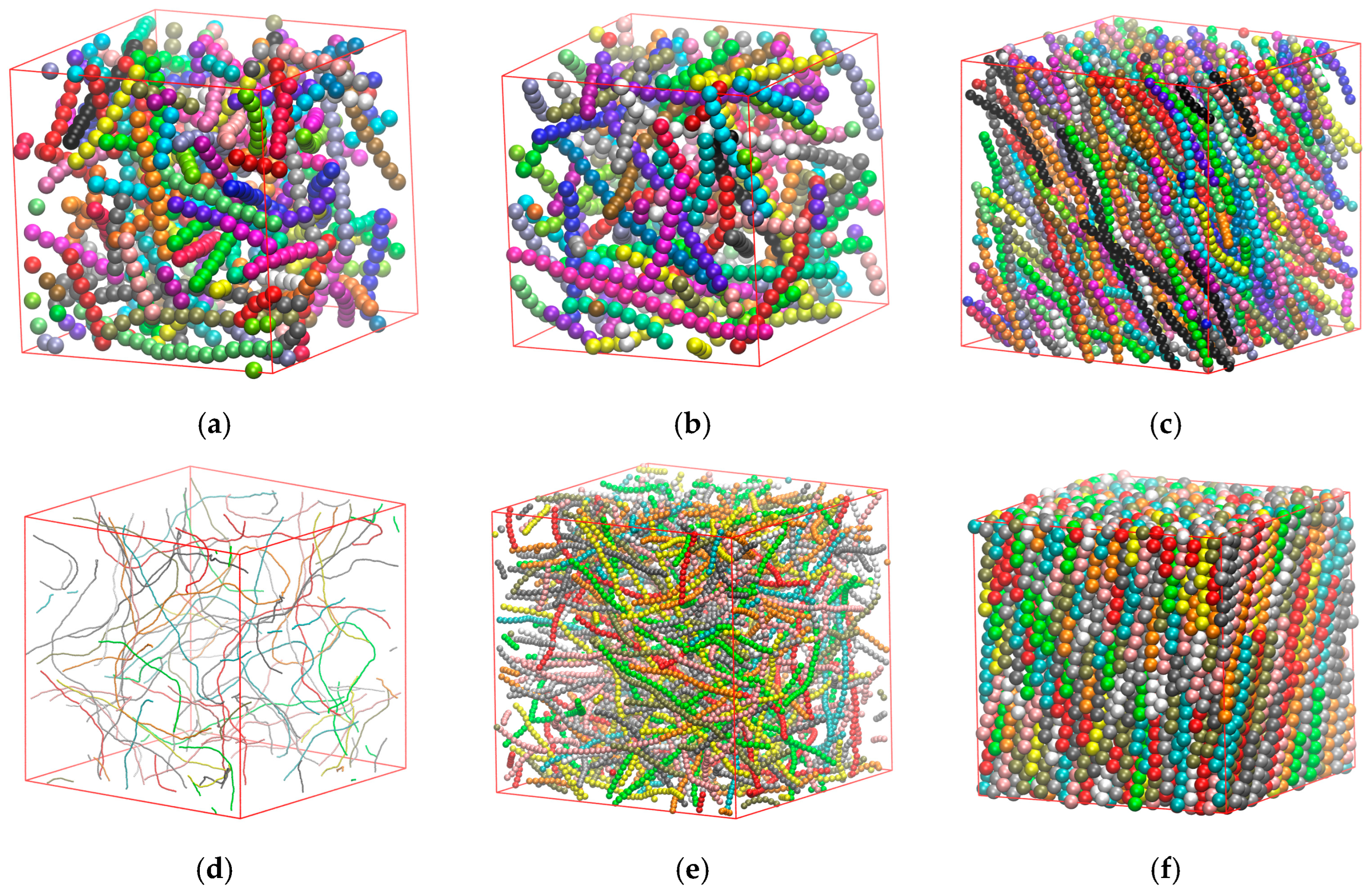
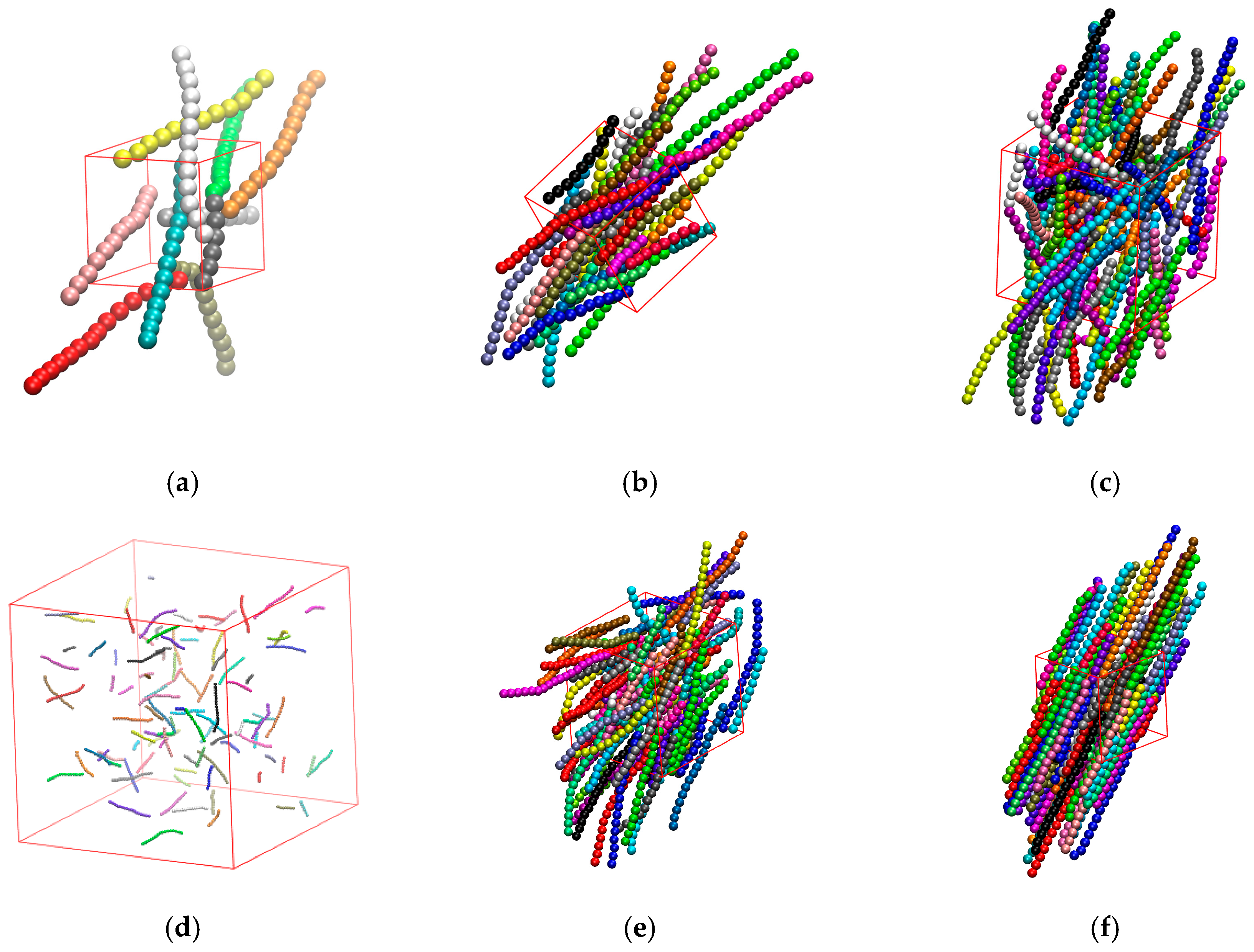
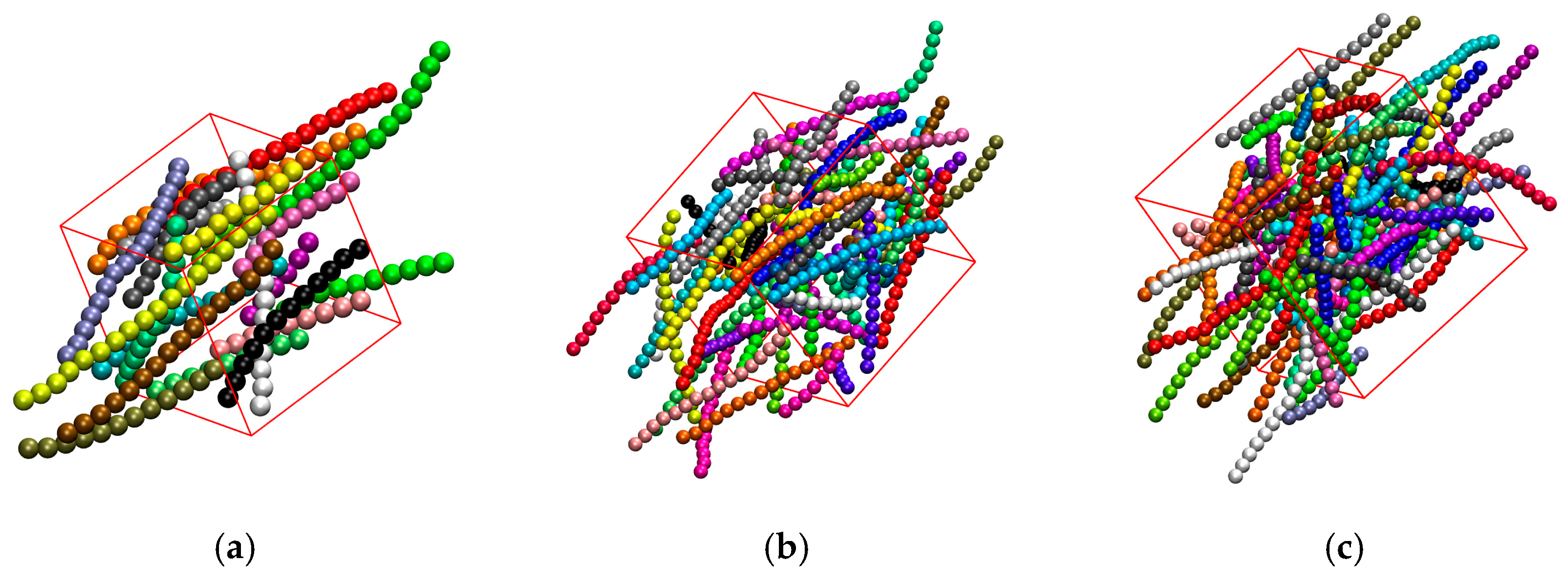
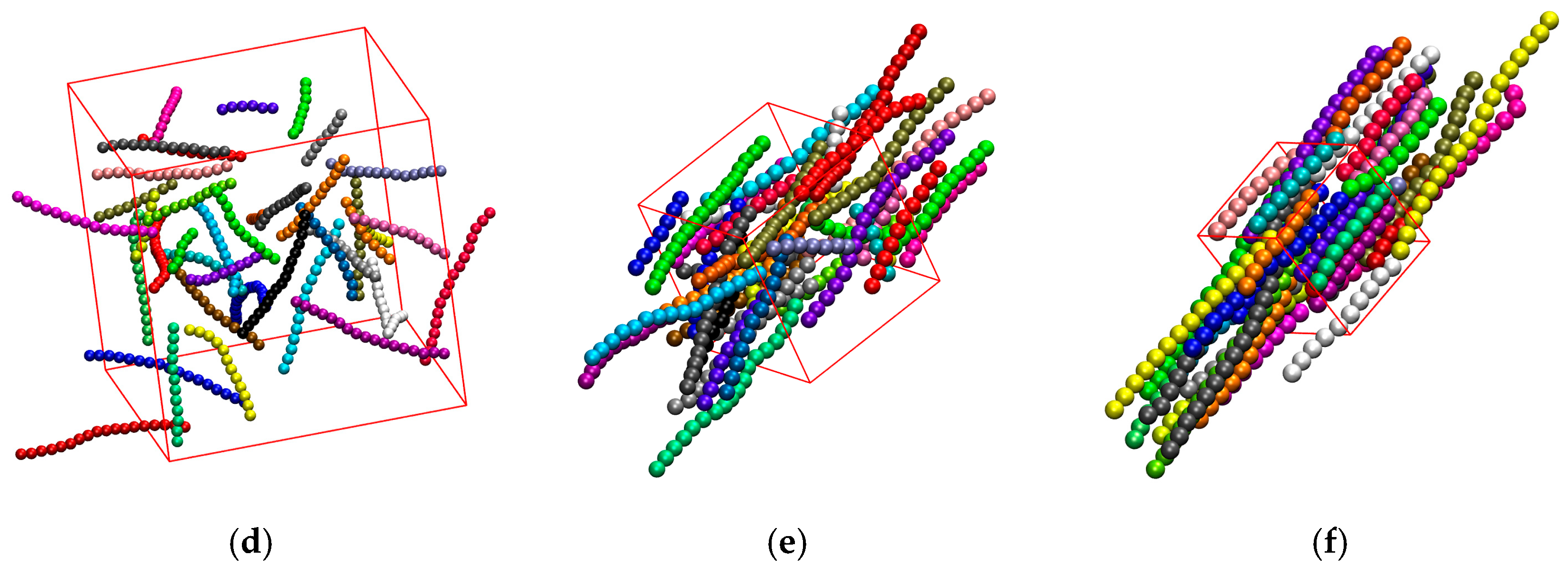
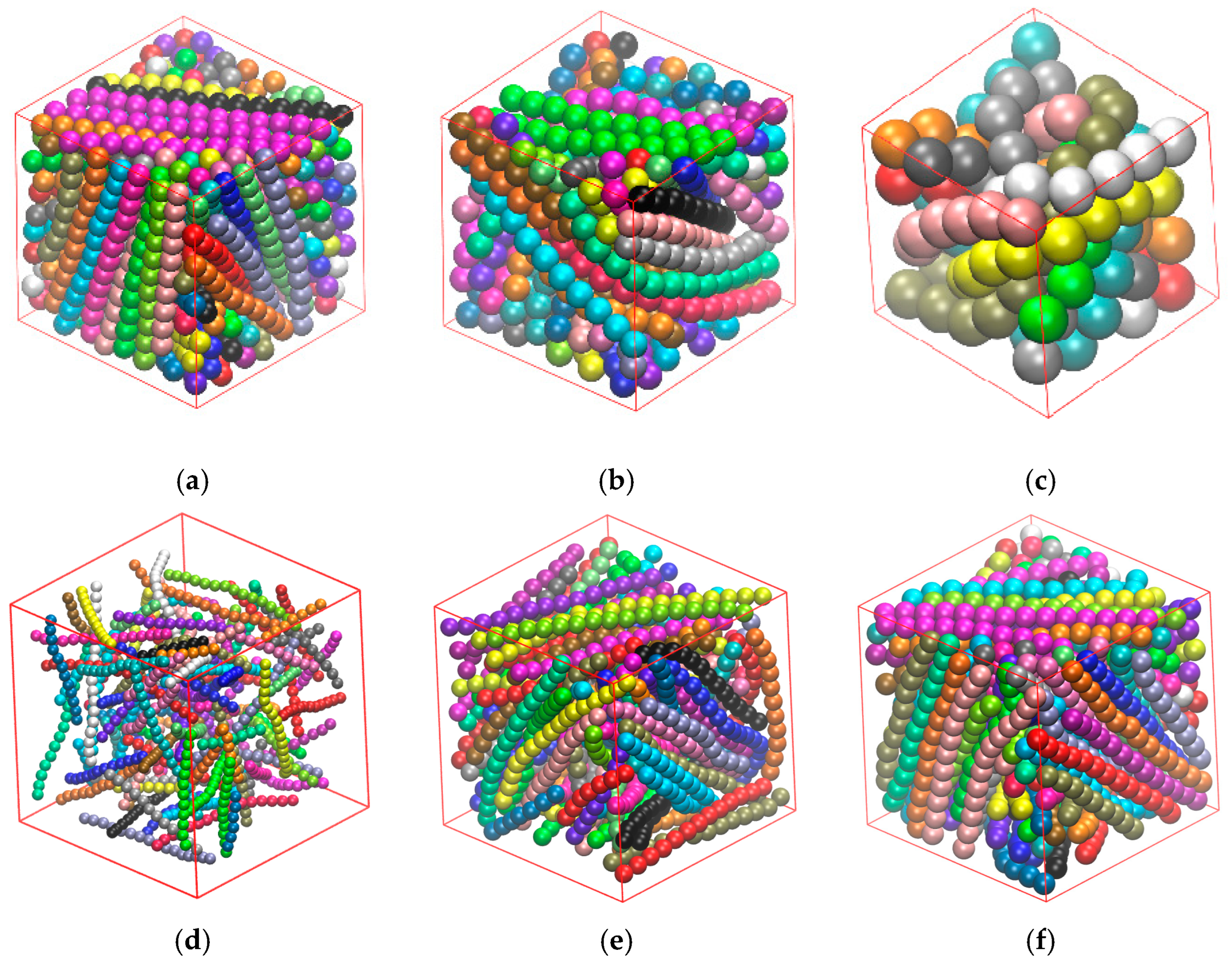
| Case | ||||||
|---|---|---|---|---|---|---|
| (a) | 0.40 | 0.524 | 1 | 11.62 | 9.40 | 10.92 (0.40); 11.00 (0.52) |
| (b) | 0.40 | 0.552 | 0.6 | 10.01 | 7.30 | 10.92 (0.40); 11.01 (0.55) |
| (c) | 0.40 | 0.740 | 0.1 | 5.39 | 2.30 | 10.92 (0.40); |
| (d) | 0.05 | 0.057 | 1 | 23.25 | 10.61 | 10.61 (0.05) |
| (e) | 0.20 | 0.247 | 1 | 14.64 | 10.63 | 10.68 (0.20); 10.77 (0.25) |
| (f) | 0.35 | 0.453 | 1 | 12.16 | 10.57 | 10.90 (0.35); 10.98 (0.45) |
Disclaimer/Publisher’s Note: The statements, opinions and data contained in all publications are solely those of the individual author(s) and contributor(s) and not of MDPI and/or the editor(s). MDPI and/or the editor(s) disclaim responsibility for any injury to people or property resulting from any ideas, methods, instructions or products referred to in the content. |
© 2025 by the authors. Licensee MDPI, Basel, Switzerland. This article is an open access article distributed under the terms and conditions of the Creative Commons Attribution (CC BY) license (https://creativecommons.org/licenses/by/4.0/).
Share and Cite
Yan, B.; Martínez-Fernández, D.; Foteinopoulou, K.; Karayiannis, N.C. Molecular Simulation of the Isotropic-to-Nematic Transition of Rod-like Polymers in Bulk and Under Confinement. Polymers 2025, 17, 1703. https://doi.org/10.3390/polym17121703
Yan B, Martínez-Fernández D, Foteinopoulou K, Karayiannis NC. Molecular Simulation of the Isotropic-to-Nematic Transition of Rod-like Polymers in Bulk and Under Confinement. Polymers. 2025; 17(12):1703. https://doi.org/10.3390/polym17121703
Chicago/Turabian StyleYan, Biao, Daniel Martínez-Fernández, Katerina Foteinopoulou, and Nikos Ch. Karayiannis. 2025. "Molecular Simulation of the Isotropic-to-Nematic Transition of Rod-like Polymers in Bulk and Under Confinement" Polymers 17, no. 12: 1703. https://doi.org/10.3390/polym17121703
APA StyleYan, B., Martínez-Fernández, D., Foteinopoulou, K., & Karayiannis, N. C. (2025). Molecular Simulation of the Isotropic-to-Nematic Transition of Rod-like Polymers in Bulk and Under Confinement. Polymers, 17(12), 1703. https://doi.org/10.3390/polym17121703