
Experimentally and Modeling Assessment of Parameters Affecting Grinding Aid-Containing Cement–PCE Compatibility: CRA, MARS and AOMA-ANN Methods

Abstract
1. Introduction
- (i)
- Evaluation in Terms of the Purpose of Using Metaheuristics in ANNs: When the studies listed in Table 1 are evaluated in terms of the purpose of using metaheuristics with ANNs, metaheuristics were shown to be used in the training of ANNs in the vast majority of studies. In such studies, the optimal values of the weights and biases utilized in the ANN model are identified via metaheuristic algorithms. However, such applications typically result in increased computational times compared to back-propagation algorithms. This is due to the fact that back-propagation algorithms reduce the error obtained in each iteration by back-propagation, whereas the process followed by metaheuristics is a stochastic process. This increases the time required to obtain a lower error. Consequently, in this study, instead of using metaheuristics in training, we used metaheuristic algorithms in the optimization of the network architecture. The design of network architectures is typically user-driven and is often conducted through a trial-and-error process, which can result in the creation of suboptimal network architectures.
- (ii)
- Evaluation in Terms of the Metaheuristic Algorithms Used: Upon evaluation of the studies listed in Table 1 in terms of the metaheuristic algorithms employed, it becomes evident that a number of the studies utilize algorithms that are relatively outdated, including Genetic Algorithm (GA), Particle Swarm Optimization Algorithm (PSO), and Differential Evolution (DE). In addition, meta-heuristic algorithms such as Biogeography-Based Optimization (BBO), Covariance Matrix Adapted Evolution Strategy Algorithm (CMAES), Adam Optimizer, Water Cycle Algorithm (WCA), Sine Cosine Algorithm (SCA, 2016), Cuttlefish Optimization Algorithm (CFOA), Electromagnetic Field Optimization (EFO), Runge–Kutta Optimization (RUN), Whale Optimization Algorithm (WOA), Salp Swarm Algorithm (SSA), Grey Wolf Optimizer (GWO), Harris Hawks Optimization (HHO), Slime Mould Algorithm (SMA), Beta Differential Evolution–Improve Particle Swarm Optimization Algorithm (BDE-IPSO), Fruit Fly Optimization Algorithm (FOA), Lion Swarm Optimization Algorithm (LSO), Sparrow Search Algorithm (SSA), Fire Fly Algorithm (FFA), Particle Swarm Optimization Algorithm with Two Differential Mutations (PSOTD) were used in these studies.
- (iii)
- Evaluation in Terms of Input Parameter Reduction Process: Upon analysis of the studies listed in Table 1 regarding the aim of reducing ANN input parameters, no study on reducing input parameters could be identified in recent ANN modeling studies on cementitious systems.
- (iv)
- Evaluation in Terms of the Proposed Metaheuristic Algorithm: When the studies listed in Table 1 are evaluated in terms of the proposed metaheuristic algorithm, it is evident that a comparison between the metaheuristic algorithms utilized cannot be made, as a significant number of studies employ only a single algorithm. It is observed that the GA, EFO, RUN, LSO, and PSOTD algorithms are proposed for hybrid ANNs in the studies where a comparison is made.

| Reference | Year | Purpose of Using Metaheuristics in ANNs | List of the Metaheuristic Algorithms Employed, Along with the Year in Which They Were First Utilized. | Is There an Input Parameter Reduction Process? | Proposed Metaheuristic Algorithm (If More Than One Algorithm Is Used) |
|---|---|---|---|---|---|
| [28] | 2024 | Training of ANN | BBO (2008) | N/A | N/A |
| [29] | 2024 | Training of ANN | PSO (1995) | N/A | N/A |
| [30] | 2023 | ANN hyperparameter optimization | CMAES (2001), GA (1989), PSO (1995) | N/A | GA |
| [31] | 2023 | Training of ANN | PSO (1995) | N/A | N/A |
| [32] | 2023 | DNN hyperparameter optimization | Adam Optimizer (2015) | N/A | N/A |
| [33] | 2023 | Training of ANN | WCA (2012), SCA (2016), CFOA (2019), EFO (2016) | N/A | EFO |
| [34] | 2023 | Training of ANN | RUN (2021), WOA (2016), SSA (2017), GWO, HHO (2019), SMA (2020) | N/A | RUN |
| [35] | 2023 | Training of ANN | BDE-IPSO (2022) | N/A | N/A |
| [36] | 2023 | Training of ANN | PSO (1995), FOA (2012), LSO (2018) and SSA (2020) | N/A | LSO |
| [37] | 2022 | Training of ANN | GA (1989) | N/A | N/A |
| [38] | 2022 | Training of ANN | FFA (2009) | N/A | N/A |
| [39] | 2022 | ANN hyperparameter optimization | PSO (1995) | N/A | N/A |
| [40] | 2022 | Training of ANN | DE (1997), PSO (1995), PSOTD (2017) | N/A | PSOTD |
- (i)
- The input parameter reduction process has not been previously employed in cement systems: The input parameter reduction process utilized in this study is an optimization process in which input parameters of low importance are removed from the model, resulting in models with reduced complexity and an enhanced fit to the data.
- (ii)
- The metaheuristic algorithms used in this study have not been used in previous recent studies: Gaining–Sharing Knowledge (GSK)-based, JAYA, Symbiotic Organisms Search (SOS), Teaching–Learning-Based Artificial Bee Colony (TLABC), and Teaching–Learning-Based Optimization Algorithm (TLBO) algorithms, which will be used in the optimization of ANN architecture in this study, have not been used and their performance has not been tested.
2. Materials and Methods
2.1. Materials
2.2. Method
3. Methodology of Modeling
3.1. Development of Models
3.2. Classic Regression Analysis (CRA)
3.3. Multivariate Adaptive Regression Splines (MARS)
3.4. Artificial Neural Networks with an Architecture Optimized by Metaheuristic Algorithms (AOMA-ANN)
4. Assessment of Experimental Results
5. Evaluation of Modeling Results
5.1. Classical Regression Analysis and MARS Results
5.2. ANN Modeling Results
- Version 1—AOMA-ANN (AIP): A model that takes into account all of the defined input parameters and optimizes the number of intermediate layers, the number of neurons in the intermediate layers, and the type of activation functions used in the layers from the ANN hypermeters.
- Version 2—AOMA-ANN (ONIP): A model that, in addition to the capabilities of version 1, can reduce the input parameters used to reduce the prediction error.
5.3. Comparing Modeling Results
5.4. Modeling Limitations
6. Conclusions
- Except for TEA, the flow performance of the mixtures was adversely affected by the increase in GA usage. This negative impact was attributed to a reduction in PCE adsorption and an increase in fine particles. Mixtures containing TEA exhibited the lowest flow performance.
- The AOMA-ANN (ONIP) model demonstrated superior performance, evidenced by their achieving the lowest error values (highest NS values) for both Marsh funnel flow time and mini-slump. The AOMA-ANN(ONIP) process systematically determined the input parameters required for error minimization, removing some input parameters that could compromise network performance without additional statistical analysis.
- Among the metaheuristic search algorithms used in the AOMA-ANN (AIP) model, the most effective algorithms in terms of hyperparameter optimization are the TLABC and JAYA algorithms, while the most effective algorithms in the AOMA-ANN (ONIP) model are the TLABC and TLBO algorithms.
- The models developed with the MARS method were significantly better in terms of their Marsh funnel flow time and mini-slump values than those derived from CRA equations. The error values of the MARS models were notably lower than those of CRA equations.
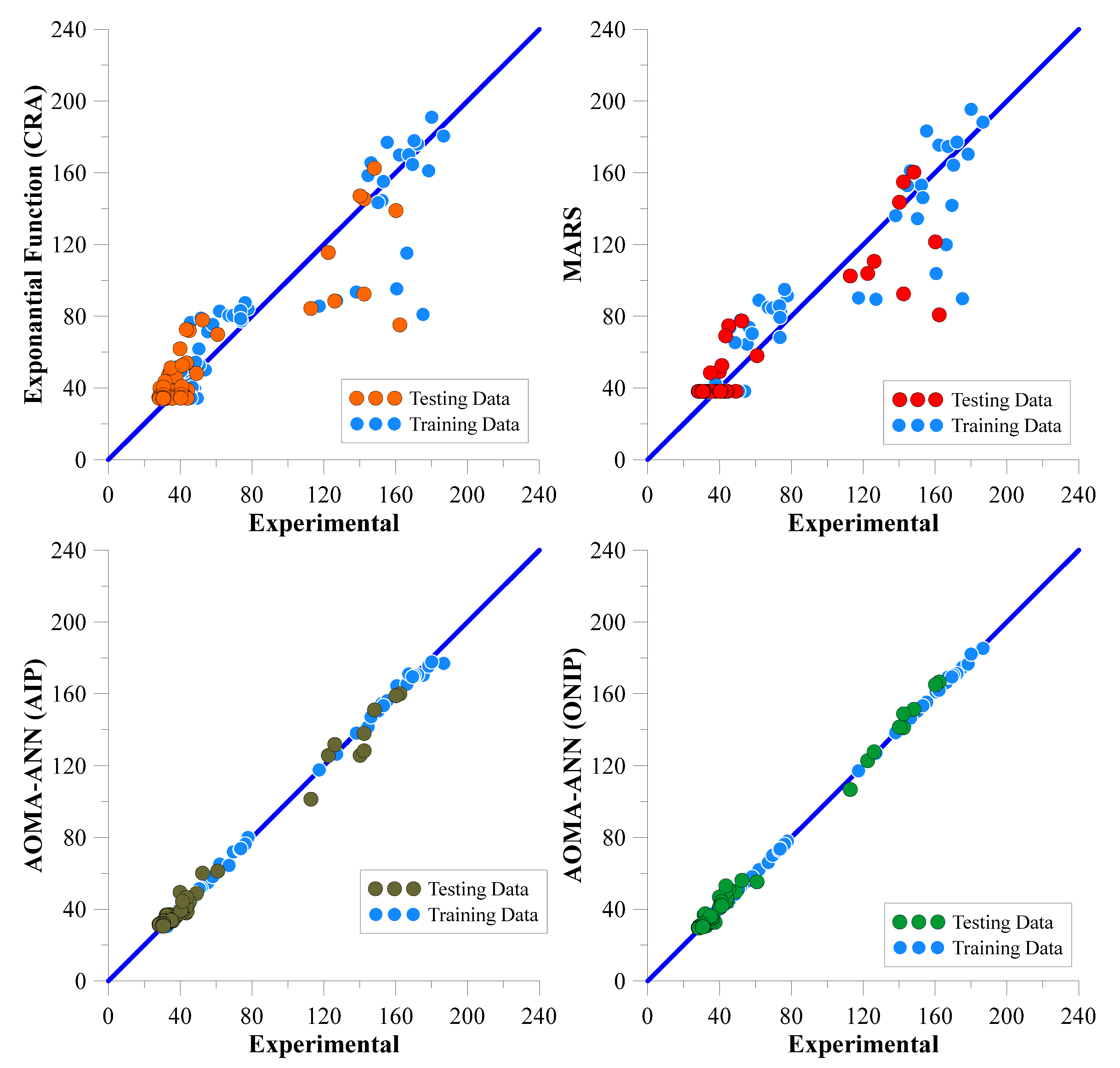
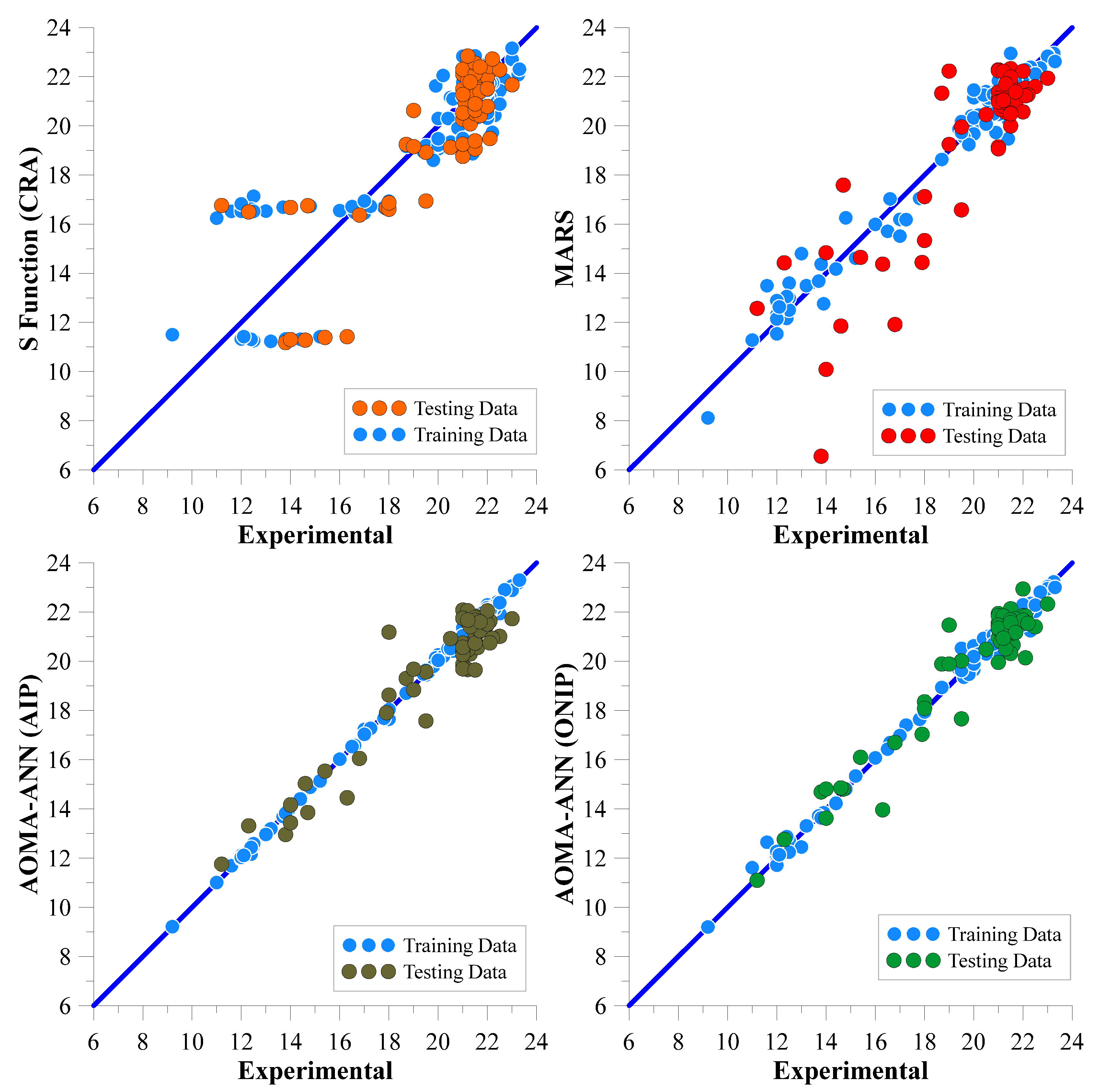
- The Marsh funnel flow time and mini-slump models created with AOMA-ANN(ONIP) exhibited the lowest scatter and accordingly were shown to have the best performance. Their predictive power surpassed that of other models.
- The AOMA-ANN model, utilized for the first time in the statistical modeling of the experimental data in this study, emerged as the most suitable data-modeling method. Predictions from this model are expected to yield comparable results, reducing the application time, materials, and labor required for extensive Marsh funnel experiments.
Author Contributions
Funding
Institutional Review Board Statement
Data Availability Statement
Acknowledgments
Conflicts of Interest
Nomenclature
| AI | Artificial Intelligence |
| ANN | Artificial Neural Network |
| CNN | Convolutional Neural Network |
| CO2 | Carbon Dioxide |
| CRA | Classical Regression Analysis |
| DEG | Diethylene Glycol |
| DEIPA | Diethanol isopropanol amine |
| EG | Ethylene glycol |
| LF | Linear Regression Function |
| MAE | Mean Absolute Error |
| MARS | Multivariate Adaptive Regression Splines |
| MARCH | Multiple Additive Regression Trees |
| M-TEA | Modified Triethanolamine |
| GA | Grinding Aid |
| PCE | Polycarboxylate Ether-Based Water-Reducing Admixture |
| PF | Power Regression Function |
| RF | Random Forest |
| RMSE | Root Mean Square Error |
| TEA | Triethanolamine |
| TIPA | Triisopropanolamine |
| ANN | Artificial Neural Networks |
References
- Kaya, Y. Farklı Tip Klinker Öğütme Kolaylaştırıcı Katkı Kullanımının Çimentolu Sistemlerin Özelliklerine Etkisi. Master’s Thesis, Bursa Uludag University, Bursa, Turkey, 2022. [Google Scholar]
- Kobya, V.; Kaya, Y.; Mardani-Aghabaglou, A. Effect of amine and glycol-based grinding aids utilization rate on grinding efficiency and rheological properties of cementitious systems. J. Build. Eng. 2022, 47, 103917. [Google Scholar] [CrossRef]
- Madlool, N.A.; Saidur, R.; Hossain, M.S.; Rahim, N.A. A critical review on energy use and savings in the cement industries. Renew. Sustain. Energy Rev. 2011, 15, 2042–2060. [Google Scholar] [CrossRef]
- Mardani-Aghabaglou, A. Investigation of Cement-Superplasticizer Admixture Compatibility. Ph.D Thesis, Ege University, Engineering Faculty, Civil Engineering Department, Izmir, Turkey, 2016. [Google Scholar]
- Engin, Y.; Tarhan, M.; Kumbaracıbaşı, S. Çimento endüstrisinde sürdürülebilir Üretim. In Proceedings of the Hazır Beton Kongresi, İstanbul, Turkey, 21–23 February 2013. [Google Scholar]
- Prziwara, P.; Breitung-Faes, S.; Kwade, A. Impact of grinding aids on dry grinding performance, bulk properties, and surface energy. Adv. Powder Technol. 2018, 29, 416–425. [Google Scholar] [CrossRef]
- Sun, Z.; Liu, H.; Ji, Y.; Pang, M. Influence of glycerin grinding aid on the compatibility between cement and polycarboxylate superplasticizer and its mechanism. Constr. Build. Mater. 2020, 233, 117104. [Google Scholar] [CrossRef]
- Prziwara, P.; Kwade, A. Grinding aids for dry fine grinding processes–Part I: Mechanism of action and lab-scale grinding. Powder Technol. 2020, 375, 146–160. [Google Scholar] [CrossRef]
- Mardani-Aghabaglou, A.; Ilhan, M.; Ozen, S. The effect of shrinkage reducing admixture and polypropylene fibers on drying shrinkage behaviour of concrete. Cem. Lime Concr. 2019, 24, 227–237. [Google Scholar] [CrossRef]
- Yüksel, C.; Mardani-Aghabaglou, A.; Beglarigale, A.; Yazıcı, H.; Ramyar, K.; Andiç-Çakır, Ö. Influence of water/powder ratio and powder type on alkali–silica reactivity and transport properties of self-consolidating concrete. Mater. Struct. 2016, 49, 289–299. [Google Scholar] [CrossRef]
- Aïtcin, P.C. High Performance Concrete; E&FN Spon: New York, NY, USA, 2004. [Google Scholar]
- Mardani-Aghabaglou, A.; Öztürk, H.T.; Kankal, M.; Ramyar, K. Assessment and prediction of cement paste flow behavior; Marsh-funnel flow time and mini-slump values. Constr. Build. Mater. 2021, 301, 124072. [Google Scholar] [CrossRef]
- Kobya, V.; Karakuzu, K.; Mardani, A.; Felekoğlu, B.; Ramyar, K. Combined interaction of PCE chains lengths, C3A and water content in cementitious systems. Constr. Build. Mater. 2023, 378, 131178. [Google Scholar] [CrossRef]
- Özen, S.; Altun, M.G.; Mardani-Aghabaglou, A.; Ramyar, K. Effect of main and side chain length change of polycarboxylate-ether-based water-reducing admixtures on the fresh state and mechanical properties of cementitious systems. Struct. Concr. 2021, 22, E607–E618. [Google Scholar] [CrossRef]
- Altun, M.G.; Özen, S.; Mardani-Aghabaglou, A. Effect of side chain length change of polycarboxylate-ether–based high-range water–reducing admixture on properties of cementitious systems containing fly ash. J. Mater. Civ. Eng. 2021, 33, 04021015. [Google Scholar] [CrossRef]
- Mardani-Aghabaglou, A.; Kankal, M.; Nacar, S.; Felekoğlu, B.; Ramyar, K. Assessment of cement characteristics affecting rheological properties of cement pastes. Neural Comput. Appl. 2021, 33, 12805–12826. [Google Scholar] [CrossRef]
- Liang, D.; Frederick, D.A.; Lledo, E.E.; Rosenfield, N.; Berardi, V.; Linstead, E.; Maoz, U. Examining the utility of nonlinear machine learning approaches versus linear regression for predicting body image outcomes: The US Body Project I. Body Image 2022, 41, 32–45. [Google Scholar] [CrossRef] [PubMed]
- Canga, D. Use of Mars data mining algorithm based on training and test sets in determining carcass weight of cattle in different Breeds. J. Agric. Sci. 2022, 28, 259–268. [Google Scholar]
- Topçu, İ.B.; Karakurt, C.; Saridemir, M. Farklı Puzolanlarla Üretilmiş Çimentoların Dayanım Gelişiminin Yapay Sinir Ağlarıyla Tahmini. Eskişehir Osman. Üniversit. Mühendislik Mimar. Fakült. Dergisi 2009, 22, 113–122. [Google Scholar]
- Cheng, M.Y.; Cao, M.T. Estimating strength of rubberized concrete using evolutionary multivariate adaptive regression splines. J. Civ. Eng. Manag. 2016, 22, 711–720. [Google Scholar] [CrossRef]
- Zhang, G.; Hamzehkolaei, N.S.; Rashnoozadeh, H.; Band, S.S.; Mosavi, A. Reliability assessment of compressive and splitting tensile strength prediction of roller compacted concrete pavement: Introducing MARS-GOA-MCS. Int. J. Pavement Eng. 2022, 23, 5030–5047. [Google Scholar] [CrossRef]
- Topçu, İ.B.; Uygunoğlu, T.; Sivri, M. Puzolanlarin Beton Basinç Dayanimina Etkisinin Yapay Sinir Ağlariyla İncelenmesi. Yapı Teknol. Elektron. Derg. 2016, 2, 1–10. [Google Scholar]
- Ashrafian, A.; Shokri, F.; Amiri, M.J.T.; Yaseen, Z.M.; Rezaie-Balf, M. Compressive strength of Foamed Cellular Lightweight Concrete simulation: New development of hybrid artificial intelligence model. Constr. Build. Mater. 2020, 230, 117048. [Google Scholar] [CrossRef]
- Gholampour, A.; Mansouri, I.; Kisi, O.; Ozbakkaloglu, T. Evaluation of mechanical properties of concretes containing coarse recycled concrete aggregates using multivariate adaptive regression splines (MARS), M5 model tree (M5Tree), and least squares support vector regression (LSSVR) models. Neural Comput. Appl. 2020, 32, 295–308. [Google Scholar] [CrossRef]
- Kaveh, A.; Hamze-Ziabari, S.M.; Bakhshpoori, T.A. Estimating drying shrinkage of concrete using a multivariate adaptive regression splines approach. Int. J. Optim. Civil Eng 2018, 8, 181–194. [Google Scholar]
- Kaveh, A.; Bakhshpoori, T.; Hamze-Ziabari, S.M. M5′and Mars based prediction models for properties of self-compacting concrete containing fly ash. Period. Polytech. Civ. Eng. 2018, 62, 281–294. [Google Scholar] [CrossRef]
- Zhang, J.; Ma, G.; Huang, Y.; Aslani, F.; Nener, B. Modelling uniaxial compressive strength of lightweight self-compacting concrete using random forest regression. Constr. Build. Mater. 2019, 210, 713–719. [Google Scholar] [CrossRef]
- Kazemi, R. A hybrid artificial intelligence approach for modeling the carbonation depth of sustainable concrete containing fly ash. Sci. Rep. 2024, 14, 11948. [Google Scholar] [CrossRef]
- Zhang, J.; Li, T.; Yao, Y.; Hu, X.; Zuo, Y.; Du, H.; Yang, J. Optimization of mix proportion and strength prediction of magnesium phosphate cement-based composites based on machine learning. Constr. Build. Mater. 2024, 411, 134738. [Google Scholar] [CrossRef]
- Aydın, Y.; Cakiroglu, C.; Bekdaş, G.; Işıkdağ, Ü.; Kim, S.; Hong, J.; Geem, Z.W. Neural Network Predictive Models for Alkali-Activated Concrete Carbon Emission Using Metaheuristic Optimization Algorithms. Sustainability 2023, 16, 142. [Google Scholar] [CrossRef]
- Ahmadi, M.; Kioumarsi, M. Predicting the elastic modulus of normal and high strength concretes using hybrid ANN-PSO. Mater. Today Proc. 2023, in press. [Google Scholar] [CrossRef]
- Choi, J.H.; Kim, D.; Ko, M.S.; Lee, D.E.; Wi, K.; Lee, H.S. Compressive strength prediction of ternary-blended concrete using deep neural network with tuned hyperparameters. J. Build. Eng. 2023, 75, 107004. [Google Scholar] [CrossRef]
- Akbarzadeh, M.R.; Ghafourian, H.; Anvari, A.; Pourhanasa, R.; Nehdi, M.L. Estimating Compressive Strength of Concrete Using Neural Electromagnetic Field Optimization. Materials 2023, 16, 4200. [Google Scholar] [CrossRef]
- Biswas, R.; Kumar, M.; Singh, R.K.; Alzara, M.; El Sayed, S.B.A.; Abdelmongy, M.; Yosri, A.M.; Yousef, S.E.A.S. A novel integrated approach of RUNge Kutta optimizer and ANN for estimating compressive strength of self-compacting concrete. Case Stud. Constr. Mater. 2023, 18, e02163. [Google Scholar] [CrossRef]
- Yang, L.; Lai, B.; Xu, R.; Hu, X.; Su, H.; Cusatis, G.; Shi, C. Prediction of alkali-silica reaction expansion of concrete using artificial neural networks. Cem. Concr. Compos. 2023, 140, 105073. [Google Scholar] [CrossRef]
- Mei, X.; Li, C.; Sheng, Q.; Cui, Z.; Zhou, J.; Dias, D. Development of a hybrid artificial intelligence model to predict the uniaxial compressive strength of a new aseismic layer made of rubber-sand concrete. Mech. Adv. Mater. Struct. 2023, 30, 2185–2202. [Google Scholar] [CrossRef]
- Hashmi, A.F.; Ayaz, M.; Bilal, A.; Shariq, M.; Baqi, A. GA-based hybrid ANN optimization approach for the prediction of compressive strength of high-volume fly ash concrete mixes. Asian J. Civ. Eng. 2023, 24, 1115–1128. [Google Scholar] [CrossRef]
- Aggarwal, Y.; Aggarwal, P.; Sihag, P.; Kumar, A. Evaluation and Estimation of Compressive Strength of Concrete Using Hybrid Modeling Techniques. Iran. J. Sci. Technol. Trans. Civ. Eng. 2022, 46, 3131–3145. [Google Scholar] [CrossRef]
- Tran, V.Q.; Giap, V.L.; Vu, D.P.; George, R.C.; Ho, L.S. Application of machine learning technique for predicting and evaluating chloride ingress in concrete. Front. Struct. Civ. Eng. 2022, 16, 1153–1169. [Google Scholar] [CrossRef]
- Hamidian, P.; Alidoust, P.; Golafshani, E.M.; Niavol, K.P.; Behnood, A. Introduction of a novel evolutionary neural network for evaluating the compressive strength of concretes: A case of Rice Husk Ash concrete. J. Build. Eng. 2022, 6, 105293. [Google Scholar] [CrossRef]
- Mardani-Aghabaglou, A.; Felekoğlu, B.; Ramyar, K. Effect of false set related anomalies on rheological properties of cement paste mixtures in the presence of high range water reducing admixture. Struct. Concr. 2021, 22, E619–E633. [Google Scholar] [CrossRef]
- EN 197-1; Cement: Composition, Specifications and Conformity Criteria, Part 1: Common Cements. European Committee for Standardization: Bruxelles, Belgium, 2000; EN/TC51/WG 6 Rev.
- Kantro, D.L. Influence of water-reducing admixtures on properties of cement paste—A miniature slump test. Cem. Concr. Aggreg. 1980, 2, 95–102. [Google Scholar] [CrossRef]
- Kobya, V.; Karakuzu, K.; Mardani, A.; Felekoğlu, B.; Ramyar, K. Effect of polycarboxylate-based water-reducing admixture chains length on portland cement-admixture compatibility. J. Sustain. Cem.-Based Mater. 2023, 13, 69–86. [Google Scholar] [CrossRef]
- Kaya, Y.; Kobya, V.; Mardani, A. Evaluation of fresh state, rheological properties, and compressive strength performance of cementitious system with grinding aids. J. Appl. Polym. Sci. 2024, 141, e55212. [Google Scholar] [CrossRef]
- Shiau, J.; Lai, V.Q.; Keawsawasvong, S. Multivariate adaptive regression splines analysis for 3D slope stability in anisotropic and heterogenous clay. J. Rock Mech. Geotech. Eng. 2023, 15, 1052–1064. [Google Scholar] [CrossRef]
- Gnanasivam, S.; Tveter, D.; Dinh, N. Performance Evaluation of Network Intrusion Detection Using Machine Learning. In Proceedings of the 2024 IEEE International Conference on Consumer Electronics (ICCE), Las Vegas, NV, USA, 6–8 January 2024; IEEE: Piscataway, NJ, USA, 2024; pp. 1–6. [Google Scholar]
- Chowdhury, M.d.S. Comparison of accuracy and reliability of random forest, support vector machine, artificial neural network and maximum likelihood method in land use/cover classification of urban setting. Environ. Chall. 2024, 14, 100800. [Google Scholar] [CrossRef]
- Öztürk, N.; Şentürk, H.B.; Gündoğdu, A.; Duran, C. Modeling of Co(II) adsorption by artificial bee colony and genetic algorithm. Membr. Water Treat. 2018, 9, 363–371. [Google Scholar] [CrossRef]
- Uzlu, E.; Akpınar, A.; Özturk, H.T.; Nacar, S.; Kankal, M. Estimates of hydroelectric generation using neural networks with the artificial bee colony algorithm for Turkey. Energy 2014, 69, 638–647. [Google Scholar] [CrossRef]
- Friedman, J.H. Multivariate adaptive regression splines (with Discussion). Ann. Stat. 1991, 19, 102–112. [Google Scholar] [CrossRef]
- Jēkabsons, G. ARESLab Version 1.13.0. 2016. Available online: http://www.cs.rtu.lv/jekabsons/regression.html (accessed on 21 June 2023).
- Mohamed, A.W.; Hadi, A.A.; Mohamed, A.K. Gaining-sharing knowledge based algorithm for solving optimization problems: A novel nature-inspired algorithm. Int. J. Mach. Learn. Cybern. 2020, 11, 1501–1529. [Google Scholar] [CrossRef]
- Venkata Rao, R. Jaya: A simple and new optimization algorithm for solving constrained and unconstrained optimization problems. Int. J. Ind. Eng. Comput. 2016, 7, 19–34. [Google Scholar] [CrossRef]
- Cheng, M.Y.; Prayogo, D. Symbiotic Organisms Search: A new metaheuristic optimization algorithm. Comput. Struct. 2014, 139, 98–112. [Google Scholar] [CrossRef]
- Chen, X.; Xu, B.; Mei, C.; Ding, Y.; Li, K. Teaching–learning–based artificial bee colony for solar photovoltaic parameter estimation. Appl. Energy 2018, 212, 1578–1588. [Google Scholar] [CrossRef]
- Rao, R.V.; Savsani, V.J.; Balic, J. Teaching-learning-based optimization algorithm for unconstrained and constrained real-parameter optimization problems. Eng. Optim. 2012, 44, 1447–1462. [Google Scholar] [CrossRef]
- Katsioti, M.; Tsakiridis, P.E.; Giannatos, P.; Tsibouki, Z.; Marinos, J. Characterization of various cement grinding aids and their impact on grindability and cement performance. Constr. Build. Mater. 2009, 23, 1954–1959. [Google Scholar] [CrossRef]
- Zunino, F.; Scrivener, K. Assessing the effect of alkanolamine grinding aids in limestone calcined clay cements hydration. Constr. Build. Mater. 2021, 266, 121293. [Google Scholar] [CrossRef]
- Kaya, Y.; Kobya, V.; Mardani, A.; Assaad, J.J. Effect of Modified Triethanolamine on Grinding Efficiency and Performance of Cementitious Materials. Talanta Open 2024, 9, 100293. [Google Scholar] [CrossRef]
- García, S.; Fernández, A.; Luengo, J.; Herrera, F. Advanced nonparametric tests for multiple comparisons in the design of experiments in computational intelligence and data mining: Experimental analysis of power. Inf. Sci. 2010, 180, 2044–2064. [Google Scholar] [CrossRef]
- Wolpert, D.H.; Macready, W.G. No free lunch theorems for optimization. IEEE Trans. Evol. Comput. 1997, 1, 67–82. [Google Scholar] [CrossRef]


| Types of Cement | Zeta Potential Values | Blaine Fineness (cm2/g) | Residue on 32 µm Sieve (%) | Residue on 45 µm Sieve (%) | Residue on 60 µm Sieve (%) |
|---|---|---|---|---|---|
| Control | −12.0 | 4100 | 31.9 | 10.4 | 1.2 |
| 0.025 TEA | −8.63 | 4110 | 26.5 | 7.6 | 0.8 |
| 0.05 TEA | −5.41 | 4115 | 18.0 | 4.7 | 0.7 |
| 0.075 TEA | −8.02 | 4100 | 16.6 | 4.0 | 0.5 |
| 0.1 TEA | −9.1 | 4090 | 14.0 | 3.1 | 0.3 |
| 0.025 TIPA | −6.24 | 4100 | 24.9 | 8.2 | 0.9 |
| 0.05 TIPA | −4.8 | 4180 | 19.0 | 4.9 | 0.8 |
| 0.075 TIPA | −3.0 | 4200 | 11.7 | 2.9 | 0.5 |
| 0.1 TIPA | −2.05 | 4140 | 9.6 | 2.1 | 0.2 |
| 0.025 DEIPA | −9.23 | 4080 | 25.8 | 9.5 | 0.8 |
| 0.05 DEIPA | −7.12 | 4090 | 21.0 | 5.8 | 0.7 |
| 0.075 DEIPA | −4.56 | 4100 | 15.2 | 3.2 | 0.5 |
| 0.1 DEIPA | −3.59 | 4020 | 13.2 | 3.0 | 0.4 |
| 0.025 DEG | −8.55 | 4110 | 23.8 | 8.2 | 0.9 |
| 0.05 DEG | −7.09 | 4140 | 16.7 | 6.0 | 0.7 |
| 0.075 DEG | −3.82 | 4190 | 12.5 | 4.8 | 0.6 |
| 0.1 DEG | −4.64 | 4150 | 9.5 | 3.1 | 0.4 |
| 0.025 EG | −9.41 | 4160 | 25.4 | 9.3 | 0.9 |
| 0.05 EG | −7.84 | 4190 | 25.8 | 8.1 | 0.9 |
| 0.075 EG | −5.12 | 4180 | 22.3 | 6.2 | 0.9 |
| 0.1 EG | −4.89 | 4160 | 17.3 | 4.3 | 0.7 |
| 0.025 M-TEA-1 | −5.74 | 4120 | 24.6 | 9.0 | 0.9 |
| 0.05 M-TEA-1 | −8.35 | 4070 | 21.0 | 6.9 | 0.6 |
| 0.075 M-TEA-1 | −8.45 | 4100 | 14.8 | 3.5 | 0.4 |
| 0.1 M-TEA-1 | −7.88 | 4050 | 14.5 | 3.4 | 0.3 |
| 0.025 M-TEA-2 | −2.79 | 4080 | 28.2 | 11.2 | 1.1 |
| 0.05 M-TEA-2 | −1.76 | 4080 | 26.2 | 10.2 | 1.0 |
| 0.075 M-TEA-2 | −1.1 | 4060 | 24.4 | 9.0 | 0.9 |
| 0.1 M-TEA-2 | −0.897 | 4050 | 23.5 | 9.0 | 0.8 |
| Type of Admixture | Alkaline Content (%) (Na2O) | Density (g/cm3) | Solid Content (%) | Chloride Content (%) | pH. 25 °C | Number of Functional Groups |
|---|---|---|---|---|---|---|
| TEA | <10 | 1.095 | 50.0 | <0.1 | 10.5 | 3 |
| TIPA | <10 | 1.124 | 50.0 | <0.1 | 10.8 | 3 |
| DEIPA | <10 | 1.079 | 50.0 | <0.1 | 9.7 | 3 |
| DEG | <10 | 1.118 | 50.0 | <0.1 | 7.2 | 2 |
| EG | <10 | 1.260 | 50.0 | <0.1 | 8.2 | 2 |
| M-TEA1 | <10 | 1.206 | 50.0 | <0.1 | 5.6 | 2 |
| M-TEA2 | <10 | 1.166 | 50.0 | <0.1 | 2.6 | 2 |
| PCE | <10 | 1.097 | 36.0 | <0.1 | 3.8 | - |
| PCE/Cement Ratio | ||||||||
|---|---|---|---|---|---|---|---|---|
| Mixtures | 0.50% | 0.75% | 1% | 1.25% | 1.50% | 1.75% | 2% | |
| C | Flow time (s) | 186.7 | 77.79 | 39.82 | 36.66 ** | 36.62 | 36.41 | 36.98 |
| Mini-slump (cm) | 9.2 | 12.5 | 22.2 | 21.5 | 23.25 | 23 | 23 | |
| 0.025 TEA | Flow time (s) | - * | 175.24 | 54 | 48.09 | 48.06 | 49.06 | 49.53 |
| Mini-slump (cm) | - | 11.6 | 19.5 | 20 | 20.5 | 21 | 22 | |
| 0.05 TEA | Flow time (s) | 162.36 | 49.12 | 44.25 | 42.41 | 43.37 | 43.91 | |
| Mini-slump (cm) | - | 12.3 | 19.5 | 21 | 21.5 | 21.5 | 21.5 | |
| 0.075 TEA | Flow time (s) | - | 160.61 | 48.22 | 43.13 | 41.75 | 42.72 | 42.68 |
| Mini-slump (cm) | - | 12.4 | 20 | 22.3 | 22.4 | 22.7 | 23.3 | |
| 0.1 TEA | Flow time (s) | - | 166.25 | 50.45 | 45.22 | 43.47 | 44.53 | 44.21 |
| Mini-slump (cm) | - | 12 | 20 | 22 | 22.5 | 21.7 | 22.3 | |
| 0.025 TIPA | Flow time (s) | 142.4 | 45.12 | 33.72 | 31.88 | 31.43 | 32.13 | 32.03 |
| Mini-slump (cm) | 13.8 | 16.8 | 21 | 21.3 | 21.1 | 21.6 | 21.2 | |
| 0.05 TIPA | Flow time (s) | 152.4 | 56.5 | 37.66 | 36.62 | 35.96 | 37.01 | 36.67 |
| Mini-slump (cm) | 13.9 | 17 | 21.4 | 21.4 | 20.6 | 19.9 | 20.2 | |
| 0.075 TIPA | Flow time (s) | 178.4 | 74.07 | 42.03 | 41.41 | 40.03 | 40.28 | 40.78 |
| Mini-slump (cm) | 13.2 | 16.6 | 19.5 | 20.6 | 20.6 | 21 | 21.2 | |
| 0.1 TIPA | Flow time (s) | 180.1 | 76.22 | 42.56 | 39.76 | 40.46 | 40.28 | 40.95 |
| Mini-slump (cm) | 12.5 | 16 | 20.9 | 21.6 | 21 | 21 | 21.2 | |
| 0.025 DEIPA | Flow time (s) | 155.3 | 62 | 35.53 | 34.13 | 33.34 | 33.62 | 33.12 |
| Mini-slump (cm) | - | 13 | 21 | 22 | 22.1 | 22.2 | 22 | |
| 0.05 DEIPA | Flow time (s) | 162.2 | 67.21 | 36.21 | 33.95 | 34.12 | 34.45 | 34.23 |
| Mini-slump (cm) | - | 12.5 | 19.4 | 21.3 | 22 | 22.1 | 22.1 | |
| 0.075 DEIPA | Flow time (s) | 167.3 | 69.61 | 38.1 | 34.51 | 34.14 | 34.57 | 34.85 |
| Mini-slump (cm) | - | 12 | 19.6 | 20.4 | 21.1 | 22 | 21.8 | |
| 0.1 DEIPA | Flow time (s) | 172.2 | 73.4 | 37.41 | 34.83 | 34.19 | 34.6 | 35.31 |
| Mini-slump (cm) | - | 11 | 19.8 | 20.8 | 21.4 | 21.9 | 22 | |
| 0.025 DEG | Flow time (s) | 140.2 | 43.41 | 33.6 | 32.62 | 32.97 | 32.45 | 32.75 |
| Mini-slump (cm) | 14 | 17.9 | 20.5 | 21.5 | 21.5 | 21.2 | 21.6 | |
| 0.05 DEG | Flow time (s) | 144.6 | 45.75 | 35.97 | 33.72 | 34.02 | 33.92 | 34.09 |
| Mini-slump (cm) | 14.4 | 18 | 21.5 | 21.8 | 22 | 21.9 | 22 | |
| 0.075 DEG | Flow time (s) | 150.2 | 55.37 | 38.93 | 36.41 | 36.62 | 36.34 | 36.73 |
| Mini-slump (cm) | 12.4 | 17.8 | 20.8 | 22 | 21.8 | 21.8 | 21.9 | |
| 0.1 DEG | Flow time (s) | 170.3 | 73.65 | 42.49 | 39.12 | 38.41 | 38.82 | 38.95 |
| Mini-slump (cm) | 12 | 16.5 | 19.5 | 21 | 22 | 21.8 | 21.9 | |
| 0.025 EG | Flow time (s) | 148.2 | 52.47 | 34.53 | 32.28 | 32.88 | 32.62 | 32.73 |
| Mini-slump (cm) | - | 14.7 | 18.7 | 19 | 21 | 21 | 21.2 | |
| 0.05 EG | Flow time (s) | 153.2 | 58.19 | 35.85 | 34.75 | 34.56 | 34.2 | 34.8 |
| Mini-slump (cm) | - | 14.8 | 20 | 21.5 | 21.5 | 21.7 | 22 | |
| 0.075 EG | Flow time (s) | 160.2 | 60.91 | 37.57 | 35.86 | 35.5 | 35.85 | 35.63 |
| Mini-slump (cm) | - | 14 | 19 | 21 | 21.7 | 22 | 22.1 | |
| 0.1 EG | Flow time (s) | 169.4 | 73.71 | 40.53 | 39.18 | 38.84 | 39.01 | 38.72 |
| Mini-slump (cm) | 13.7 | 18.7 | 21 | 21.2 | 21.7 | 21.4 | ||
| 0.025 M-TEA-1 | Flow time (s) | 122.5 | 39.95 | 31.59 | 31.06 | 30.87 | 30.99 | 31.02 |
| Mini-slump (cm) | 14.6 | 18 | 21.5 | 21.7 | 21 | 21.2 | 21 | |
| 0.05 M-TEA-1 | Flow time (s) | - | 51.68 | 36 | 35.06 | 34.06 | 34.64 | 34.35 |
| Mini-slump (cm) | - | 17.25 | 21.3 | 21.5 | 22 | 21.7 | 21.7 | |
| 0.075 M-TEA-1 | Flow time (s) | - | 127.11 | 50.61 | 46.76 | 45.31 | 45.81 | 46.02 |
| Mini-slump (cm) | - | 12 | 20.5 | 21.7 | 21.7 | 21 | 21.2 | |
| 0.1 M-TEA-1 | Flow time (s) | - | 142.45 | 43.56 | 40.94 | 40.53 | 40.06 | 40.41 |
| Mini-slump (cm) | - | 11.2 | 21 | 21.5 | 22 | 21.5 | 21.5 | |
| 0.025 M-TEA-2 | Flow time (s) | 112.8 | 34.9 | 28.75 | 28.81 | 28.19 | 28.37 | 28.53 |
| Mini-slump (cm) | 15.4 | 18 | 21.5 | 22 | 23 | 22.5 | 22.2 | |
| 0.05 M-TEA-2 | Flow time (s) | 117.4 | 37.8 | 29.56 | 29.44 | 29.21 | 29.56 | 29.63 |
| Mini-slump (cm) | 15.2 | 18 | 20 | 22.5 | 21 | 21.3 | 21 | |
| 0.075 M-TEA-2 | Flow time (s) | 126.1 | 41.3 | 30.81 | 30.63 | 30.43 | 30.21 | 30.72 |
| Mini-slump (cm) | 16.3 | 19.5 | 22.1 | 21.5 | 21.3 | 21.7 | 21.2 | |
| 0.1 M-TEA-2 | Flow time (s) | 138.1 | 48.7 | 34.41 | 32.35 | 32.63 | 32.42 | 32.78 |
| Mini-slump (cm) | 12.1 | 17 | 21 | 21.5 | 21.3 | 21.7 | 21.5 | |
| Design Variable | Lower Limit | Upper Limit | Increment | Number of Possible Values |
|---|---|---|---|---|
| D1: Number of neurons in the first hidden layer | 2 | 30 | 1 | 29 |
| D2: Number of neurons in the second hidden layer | 0 | 30 | 1 | 31 |
| D3: Activation function in the first hidden layer | {purelin, tansig, logsig, elliotsig, hardlim, hardlims, satlin, satlins, poslin, tribas, radbasi, radbasn} | 12 | ||
| D4: Activation function in the second hidden layer | 12 | |||
| D5: Output layer activation function | 12 | |||
| D6 *: 1. Decision variable for utilization of input data | 0 | 1 | 1 | 2 |
| … | … | … | … | … |
| D(6+NDV) * NDV. Decision variable for utilization of input data | 0 | 1 | 1 | 2 |
| Algorithm | Reference | Settings |
|---|---|---|
| GSK | [53] | Population size = 100, p = 0.1, = 0.5, = 0.9, K = 10 |
| JAYA | [54] | Population size = 50 |
| SOS | [55] | Ecosystem size = 50 |
| TLABC | [56] | Number of food sources (NP) = 50, limit = 200, Scale factor (F) = rand |
| TLBO | [57] | Population size = 50 |
| Models | |||||||
|---|---|---|---|---|---|---|---|
| Linear Function (LF) | Power Function (PF) | Exponential Function (EF) | Inverse Function (InvF) | Ln Function (LnF) | S Function (SF) | ||
| Coefficients | w0 | 0.672686 | 0.067125 | 0.129688 | −0.01604 | −0.03504 | −2.23811 |
| w1 | 0.000127 | −0.00522 | 1.578782 | −0.00051 | 0.004193 | 0.00348 | |
| w2 | −0.10709 | −0.20029 | −0.01263 | 0.009211 | −0.04366 | 0.032356 | |
| w3 | −0.07709 | −0.32749 | −1.07705 | 0.035599 | −0.05802 | 0.138471 | |
| w4 | 0.026625 | 0.08254 | −1.05479 | −0.0051 | 0.006858 | −0.03734 | |
| w5 | −0.10448 | −0.07219 | 0.312201 | −0.00568 | −0.0143 | 0.011679 | |
| w6 | 0.059809 | 0.173447 | −0.73144 | −0.02005 | 0.034241 | −0.0938 | |
| w7 | −0.57552 | −0.9488 | 0.477011 | 0.073521 | −0.2709 | 0.186458 | |
| w8 | −8.06557 | ||||||
| Models | |||||||
|---|---|---|---|---|---|---|---|
| Linear Function (LF) | Power Function (PF) | Exponential Function (EF) | Inverse Function (InvF) | Ln Function (LnF) | S Function (SF) | ||
| Coefficients | w0 | 0.3653394 | 0.905302 | −16.577439 | 0.886149 | 0.8901377 | −0.0077721 |
| w1 | 0.0324581 | 0.0124977 | 2.833863 | −0.0064834 | 0.0235283 | −0.004288 | |
| w2 | −0.0002337 | −0.0048646 | 0.0020997 | 0.0011546 | −0.0061773 | 0.0010272 | |
| w3 | −0.0294216 | −0.0256414 | −0.0026935 | −0.0049123 | −0.0016362 | 0.0096925 | |
| w4 | −0.0275952 | 0.0032983 | −0.0021603 | 0.0009593 | −0.0120337 | −0.0048578 | |
| w5 | 0.0844444 | 0.0454036 | −0.0022321 | −0.0191991 | 0.0490472 | −0.0249233 | |
| w6 | −0.0653068 | −0.0519783 | 0.0034666 | 0.0255447 | −0.0522755 | 0.0271541 | |
| w7 | 0.5895366 | 0.3988167 | −0.005128 | −0.0692647 | 0.2687517 | −0.1521553 | |
| w8 | 0.0337381 | ||||||
| Basic Functions |
|---|
| BF1 = max(0, 1 − x7) BF2 = BF1 * max(0, x2 − 0.9) BF3 = BF1 * max(0, 0.9 − x2) BF4 = BF1 * max(0, x3 + 2.05) BF5 = BF1 * max(0, −2.05 − x3) BF6 = max(0, 0.75 − x7) BF7 = BF1 * max(0, 10.8 − x6) |
| Marsh-funnel flow time = 38.149 + 70.296 * BF1 + 518.51 * BF2 + 224.02 * BF3 + 140.45 * BF4 + 18.102 * BF5 + 174.64 * BF6 − 17.882 * BF7 |
| Basic Functions |
|---|
| BF1 = C(x6|+1, 4.915, 7.2, 8.85) BF2 = C(x6|−1, 4.915, 7.2, 8.85) BF3 = C(x7|+1, 0.625, 0.75, 0.875) * C(x6|+1, 1.315, 2.63, 4.915) BF4 = C(x7|−1, 0.875, 1, 1.125) * C(x1|+1, 4050, 4080, 4085) BF5 = C(x7|−1, 0.875, 1, 1.125) * C(x1|−1, 4050, 4080, 4085) BF6 = C(x7|−1, 0.875, 1, 1.125) * C(x1|+1, 4085, 4090, 4115) BF7 = C(x7|−1, 0.875, 1, 1.125) * C(x1|−1, 4115, 4140, 4160) BF8 = C(x7|+1, 0.875, 1, 1.125) * C(x6|+1, 8.85, 10.5, 10.65) BF9 = C(x4|+1, 0.47076, 0.94152, 3.386) * C(x7|−1, 1.125, 1.25, 1.625) BF10 = C(x7|−1, 0.625, 0.75, 0.875) * C(x1|−1, 4160, 4180, 4190) BF11 = C(x4|−1, 0.47076, 0.94152, 3.386) * C(x1|+1, 4050, 4080, 4085) BF12 = C(x4|−1, 0.47076, 0.94152, 3.386) * C(x1|−1, 4050, 4080, 4085) BF13 = C(x7|+1, 0.875, 1, 1.125) * C(x5|+1, 0.555, 1.11, 1.115) BF14 = C(x7|+1, 1.125, 1.25, 1.625) BF15 = C(x4|+1, 0.47076, 0.94152, 3.386) * C(x5|+1, 1.14, 1.16, 1.18) BF16 = C(x7|+1, 0.875, 1, 1.125) * C(x3|+1, −8.56, −8.02, −4.4585) BF17 = C(x7|+1, 0.875, 1, 1.125) * C(x3|-1, −8.56, −8.02, −4.4585) BF18 = C(x7|+1, 0.625, 0.75, 0.875) * C(x3|+1, -10.55, −9.1, −8.56) BF19 = C(x7|+1, 0.625, 0.75, 0.875) * C(x3|−1, −10.55, −9.1, −8.56) BF20 = C(x5|+1, 1.115, 1.12, 1.14) BF21 = C(x5|−1, 1.115, 1.12, 1.14) |
| Mini-slump = 21.144 − 0.19824 * BF1 + 0.43059 * BF2 + 0.37666 * BF3 − 1.5606 * BF4 +0.16825 * BF5 + 1.5794 * BF6 − 0.40074 * BF7 − 1.9121 * BF8 − 1.5543 * BF9 + 0.17399 * BF10 − 0.0511 * BF11 − 0.047408 * BF12 + 7.4156 * BF13 − 1.3511 * BF14 − 63.353 * BF15 + 0.52832 * BF16 − 1.0831 * BF17 − 0.51918 * BF18 + 1.878 * BF19 − 0.11206 * BF20 − 1.7269 * BF21 |
| Model | Training Data | Testing Data | All Data | |||
|---|---|---|---|---|---|---|
| RMSE | NS | RMSE | NS | RMSE | NS | |
| LF | 30.82 | 0.490 | 28.72 | 0.423 | 30.19 | 0.477 |
| PF | 15.89 | 0.864 | 17.82 | 0.778 | 16.52 | 0.843 |
| EF | 14.86 | 0.882 | 17.29 | 0.791 | 15.65 | 0.859 |
| InvF | 16.85 | 0.848 | 19.93 | 0.722 | 17.86 | 0.817 |
| LnF | 22.60 | 0.726 | 23.24 | 0.622 | 22.80 | 0.701 |
| SF | 17.20 | 0.841 | 19.14 | 0.744 | 17.83 | 0.817 |
| MARS | 13.46 | 0.903 | 16.19 | 0.817 | 14.36 | 0.882 |
| Model | Training Data | Testing Data | All Data | |||
|---|---|---|---|---|---|---|
| RMSE | NS | RMSE | NS | RMSE | NS | |
| LF | 2.14 | 0.598 | 1.96 | 0.513 | 2.09 | 0.578 |
| PF | 1.86 | 0.696 | 1.77 | 0.601 | 1.84 | 0.674 |
| EF | 2.16 | 0.594 | 1.98 | 0.502 | 2.10 | 0.573 |
| InvF | 1.87 | 0.694 | 1.80 | 0.588 | 1.85 | 0.669 |
| LnF | 1.71 | 0.744 | 1.69 | 0.639 | 1.70 | 0.719 |
| SF | 1.65 | 0.763 | 1.79 | 0.592 | 1.70 | 0.722 |
| MARS | 0.60 | 0.968 | 1.80 | 0.587 | 1.13 | 0.878 |
| Model Type | Algorithms Friedman Scores | |||||
|---|---|---|---|---|---|---|
| GSK | JAYA | SOS | TLABC | TLBO | ||
| Marsh Funnel Flow-Time ANN Model | AOMA-ANN (AIP) | 2.95 | 3.38 | 3.24 | 2.33 | 3.10 |
| AOMA-ANN (ONIP) | 4.05 | 3.38 | 3.10 | 2.14 | 2.33 | |
| Mini-Slump ANN Model | AOMA-ANN (AIP) | 2.43 | 2.14 | 3.10 | 3.48 | 3.86 |
| AOMA-ANN (ONIP) | 3.33 | 2.57 | 3.90 | 3.02 | 2.17 | |
| Model | Method | Algorithm | Training Dataset | Testing Dataset | All Datasets | ||||||
|---|---|---|---|---|---|---|---|---|---|---|---|
| MSE | RMSE | NS | MSE | RMSE | NS | MSE | RMSE | NS | |||
| Marsh-Funnel Flow Time ANN Model | AOMA-ANN (AIP) | GSK | 1.28 | 1.13 | 0.999 | 24.80 | 4.98 | 0.983 | 8.56 | 2.93 | 0.995 |
| JAYA | 0.92 | 0.96 | 1.000 | 27.34 | 5.23 | 0.981 | 9.10 | 3.02 | 0.995 | ||
| SOS | 2.18 | 1.47 | 0.999 | 20.85 | 4.57 | 0.985 | 7.96 | 2.82 | 0.995 | ||
| TLABC | 2.20 | 1.48 | 0.999 | 17.11 | 4.14 | 0.988 | 6.81 | 2.61 | 0.996 | ||
| TLBO | 0.69 | 0.83 | 1.000 | 27.17 | 5.21 | 0.981 | 8.89 | 2.98 | 0.995 | ||
| AOMA-ANN (ONIP) | GSK | 0.35 | 0.59 | 1.000 | 15.15 | 3.89 | 0.989 | 4.94 | 2.22 | 0.997 | |
| JAYA | 0.63 | 0.80 | 1.000 | 13.17 | 3.63 | 0.991 | 4.51 | 2.12 | 0.997 | ||
| SOS | 0.49 | 0.70 | 1.000 | 17.00 | 4.12 | 0.988 | 5.60 | 2.37 | 0.997 | ||
| TLABC | 0.41 | 0.64 | 1.000 | 9.44 | 3.07 | 0.993 | 3.21 | 1.79 | 0.998 | ||
| TLBO | 0.87 | 0.93 | 1.000 | 11.06 | 3.32 | 0.992 | 4.03 | 2.01 | 0.998 | ||
| Mini-Slump ANN Model | AOMA-ANN (AIP) | GSK | 0.03 | 0.18 | 0.997 | 0.83 | 0.91 | 0.894 | 0.28 | 0.53 | 0.973 |
| JAYA | 0.02 | 0.14 | 0.998 | 0.83 | 0.91 | 0.895 | 0.27 | 0.52 | 0.974 | ||
| SOS | 0.06 | 0.25 | 0.995 | 0.75 | 0.86 | 0.905 | 0.28 | 0.53 | 0.973 | ||
| TLABC | 0.10 | 0.31 | 0.992 | 0.82 | 0.91 | 0.896 | 0.32 | 0.57 | 0.969 | ||
| TLBO | 0.04 | 0.20 | 0.997 | 0.89 | 0.94 | 0.887 | 0.31 | 0.55 | 0.971 | ||
| AOMA-ANN (ONIP) | GSK | 0.06 | 0.23 | 0.995 | 0.69 | 0.83 | 0.913 | 0.25 | 0.50 | 0.976 | |
| JAYA | 0.08 | 0.28 | 0.993 | 0.61 | 0.78 | 0.923 | 0.24 | 0.49 | 0.976 | ||
| SOS | 0.05 | 0.22 | 0.996 | 0.72 | 0.85 | 0.909 | 0.26 | 0.51 | 0.975 | ||
| TLABC | 0.09 | 0.30 | 0.992 | 0.65 | 0.81 | 0.918 | 0.27 | 0.52 | 0.974 | ||
| TLBO | 0.02 | 0.15 | 0.998 | 0.78 | 0.88 | 0.902 | 0.26 | 0.51 | 0.975 | ||
| Models | ||||||||||
|---|---|---|---|---|---|---|---|---|---|---|
| Data | Error | Classical Regression Analysis | MARS | AOMA-ANN | ||||||
| LF | PF | EF | InvF | LnF | SF | AIP | ONIP | |||
| Training | RMSE | 30.82 | 15.89 | 14.86 | 16.85 | 22.60 | 17.20 | 13.46 | 2.20 | 0.41 |
| NS | 0.490 | 0.864 | 0.882 | 0.848 | 0.726 | 0.841 | 0.903 | 0.999 | 1.000 | |
| Testing | RMSE | 28.72 | 17.82 | 17.29 | 19.93 | 23.24 | 19.14 | 16.19 | 17.11 | 9.44 |
| NS | 0.423 | 0.778 | 0.791 | 0.722 | 0.622 | 0.744 | 0.817 | 0.988 | 0.993 | |
| All | RMSE | 28.72 | 17.82 | 17.29 | 19.93 | 23.24 | 19.14 | 16.19 | 6.81 | 3.21 |
| NS | 0.423 | 0.778 | 0.791 | 0.722 | 0.622 | 0.744 | 0.817 | 0.996 | 0.998 | |
| Models | ||||||||||
|---|---|---|---|---|---|---|---|---|---|---|
| Data | Error | Classical Regression Analysis | MARS | AOMA-ANN | ||||||
| LF | PF | EF | InvF | LnF | SF | AIP | ONIP | |||
| Training | RMSE | 2.14 | 1.86 | 2.16 | 1.87 | 1.71 | 1.65 | 0.60 | 0.02 | 0.08 |
| NS | 0.598 | 0.696 | 0.594 | 0.694 | 0.744 | 0.763 | 0.968 | 0.998 | 0.993 | |
| Testing | RMSE | 1.96 | 1.77 | 1.98 | 1.80 | 1.69 | 1.79 | 1.80 | 0.83 | 0.61 |
| NS | 0.513 | 0.601 | 0.502 | 0.588 | 0.639 | 0.592 | 0.587 | 0.895 | 0.923 | |
| All | RMSE | 2.09 | 1.84 | 2.10 | 1.85 | 1.70 | 1.70 | 1.13 | 0.27 | 0.24 |
| NS | 0.578 | 0.674 | 0.573 | 0.669 | 0.719 | 0.722 | 0.878 | 0.974 | 0.976 | |
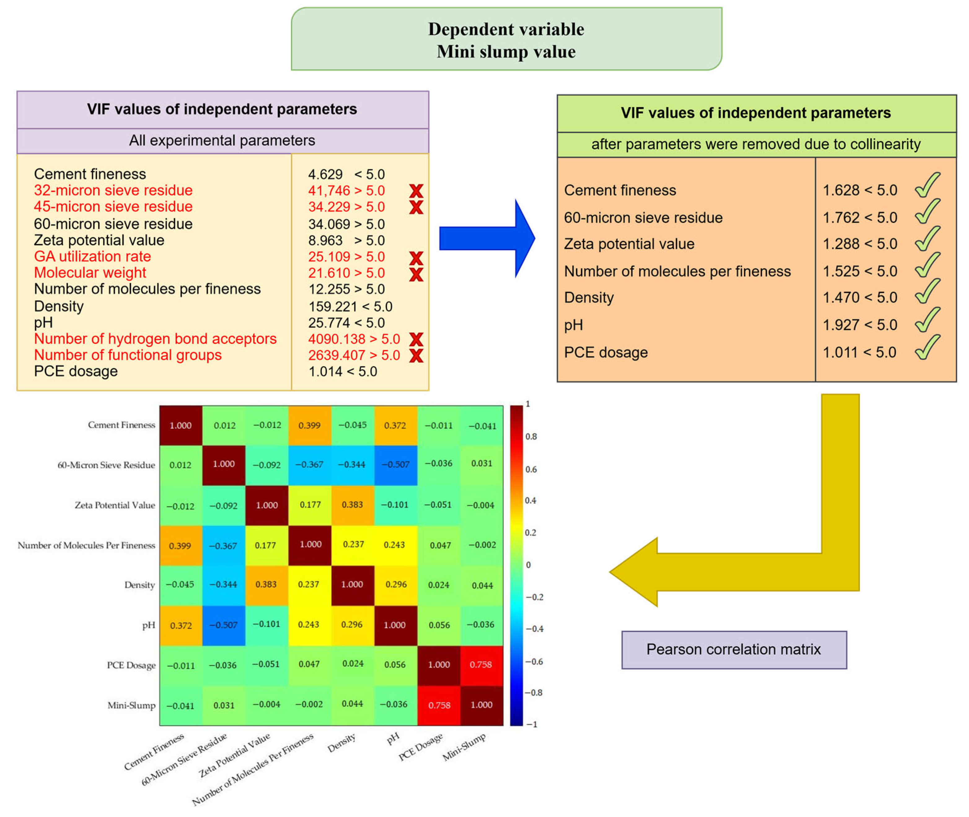
| Input Parameters | |||||||
|---|---|---|---|---|---|---|---|
| Limit | X1 | X2 | X3 | X4 | X5 | X6 | X7 |
| Minimum | 4020 | 0.2 | −12 | 0 | 0 | 0 | 0.5 |
| Maximum | 4200 | 1.2 | −0.897 | 5.830 | 1.2 | 10.8 | 2 |
| X1: Cement fineness X2: Sieve residue at 60 microns X3: Zeta potential X4: Number of molecules per fineness | X5: Density of GA X6: pH value of GA X7: PCE dosage (%) | ||||||
Disclaimer/Publisher’s Note: The statements, opinions and data contained in all publications are solely those of the individual author(s) and contributor(s) and not of MDPI and/or the editor(s). MDPI and/or the editor(s) disclaim responsibility for any injury to people or property resulting from any ideas, methods, instructions or products referred to in the content. |
© 2025 by the authors. Licensee MDPI, Basel, Switzerland. This article is an open access article distributed under the terms and conditions of the Creative Commons Attribution (CC BY) license (https://creativecommons.org/licenses/by/4.0/).
Share and Cite
Kaya, Y.; Öztürk, H.T.; Kobya, V.; Mardani, N.; Mardani, A. Experimentally and Modeling Assessment of Parameters Affecting Grinding Aid-Containing Cement–PCE Compatibility: CRA, MARS and AOMA-ANN Methods. Polymers 2025, 17, 1583. https://doi.org/10.3390/polym17111583
Kaya Y, Öztürk HT, Kobya V, Mardani N, Mardani A. Experimentally and Modeling Assessment of Parameters Affecting Grinding Aid-Containing Cement–PCE Compatibility: CRA, MARS and AOMA-ANN Methods. Polymers. 2025; 17(11):1583. https://doi.org/10.3390/polym17111583
Chicago/Turabian StyleKaya, Yahya, Hasan Tahsin Öztürk, Veysel Kobya, Naz Mardani, and Ali Mardani. 2025. "Experimentally and Modeling Assessment of Parameters Affecting Grinding Aid-Containing Cement–PCE Compatibility: CRA, MARS and AOMA-ANN Methods" Polymers 17, no. 11: 1583. https://doi.org/10.3390/polym17111583
APA StyleKaya, Y., Öztürk, H. T., Kobya, V., Mardani, N., & Mardani, A. (2025). Experimentally and Modeling Assessment of Parameters Affecting Grinding Aid-Containing Cement–PCE Compatibility: CRA, MARS and AOMA-ANN Methods. Polymers, 17(11), 1583. https://doi.org/10.3390/polym17111583