

Estimation and Prediction of the Polymers’ Physical Characteristics Using the Machine Learning Models

 ,
,  ,
,
Abstract
:1. Introduction
- Material Design and Engineering. Precise predictions of properties such as tensile strength, elasticity, and thermal conductivity empower material scientists in designing polymers with tailored attributes [5]. This facilitates the creation of innovative materials for specific applications, ranging from lightweight composites in aerospace engineering [6] to durable polymers in medical devices [7].
- Process Optimization. Understanding and predicting physical characteristics play a crucial role in optimizing manufacturing processes. For instance, predicting melt viscosity in polymer processing aids [8] in controlling the extrusion process, ensuring the production of consistent and high-quality polymer products [9].
- Quality Control in Polymer Manufacturing. The ability to predict physical characteristics is instrumental in quality control within polymer manufacturing [10]. Predictive models can assist in identifying deviations in real-time, enabling timely adjustments in the production process to maintain desired material properties.
- Environmental Impact Assessment. Predicting properties is essential in determining their biodegradability and recyclability [11]. It contributes to the assessment of a polymer’s environmental impact. This knowledge is particularly relevant in the development of sustainable materials, aligning with the growing emphasis on eco-friendly practices.
- Pharmaceutical and Medical Applications. In the field of pharmaceuticals, predicting characteristics can help to determine drug release rates from polymer matrices [12]. It is vital for designing controlled drug delivery systems. Similarly, in medical applications, predicting the mechanical properties of biocompatible polymers is crucial for developing implants and medical devices.
2. Materials and Methods
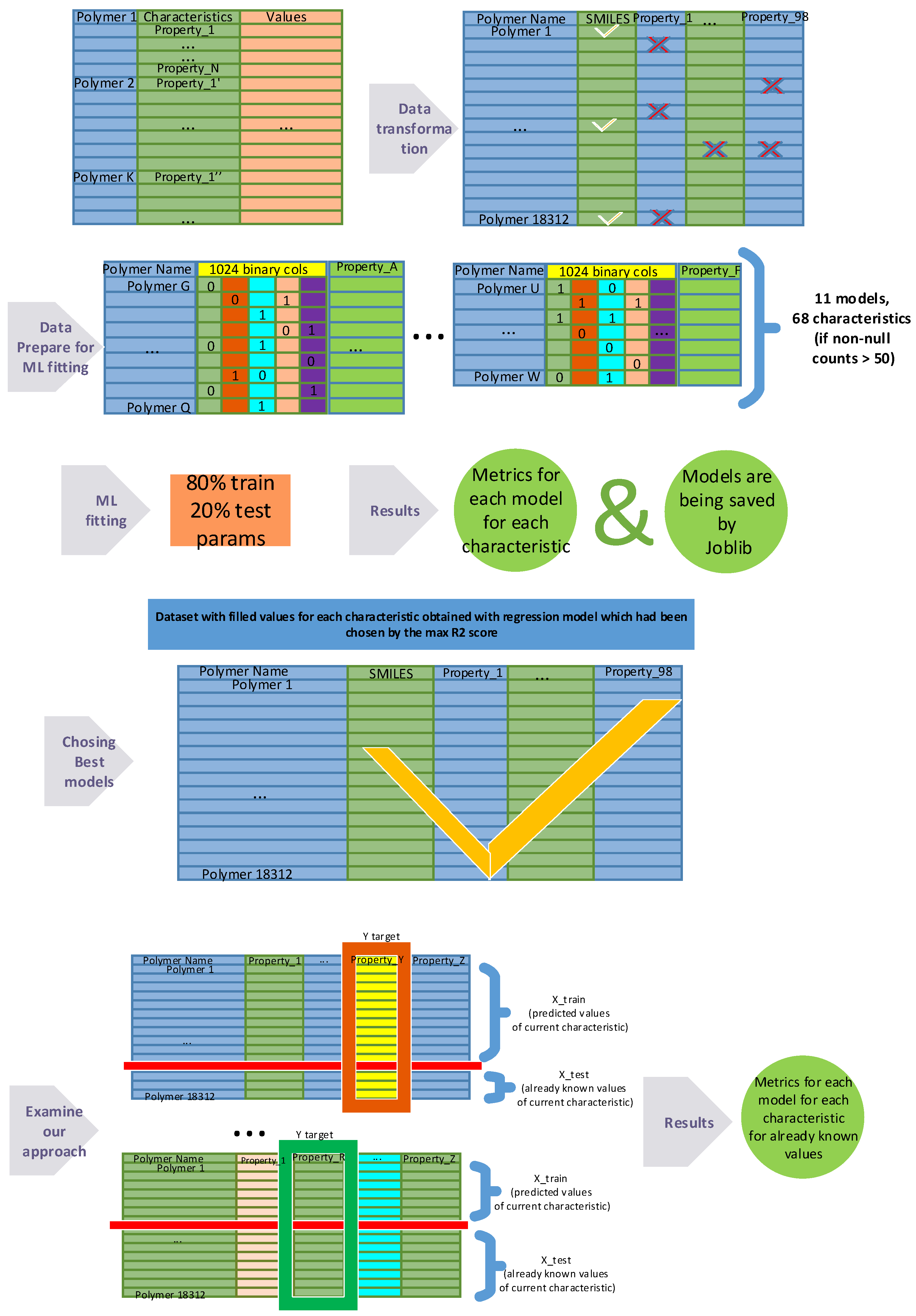
2.1. Dataset Preparation
2.2. Model Training for Predicting the Physical Characteristics of Polymer
2.3. Using Prediction Method for Imputation of Missing Values of Polymer Physical 98 Characteristics
2.4. Examination of Our Approach
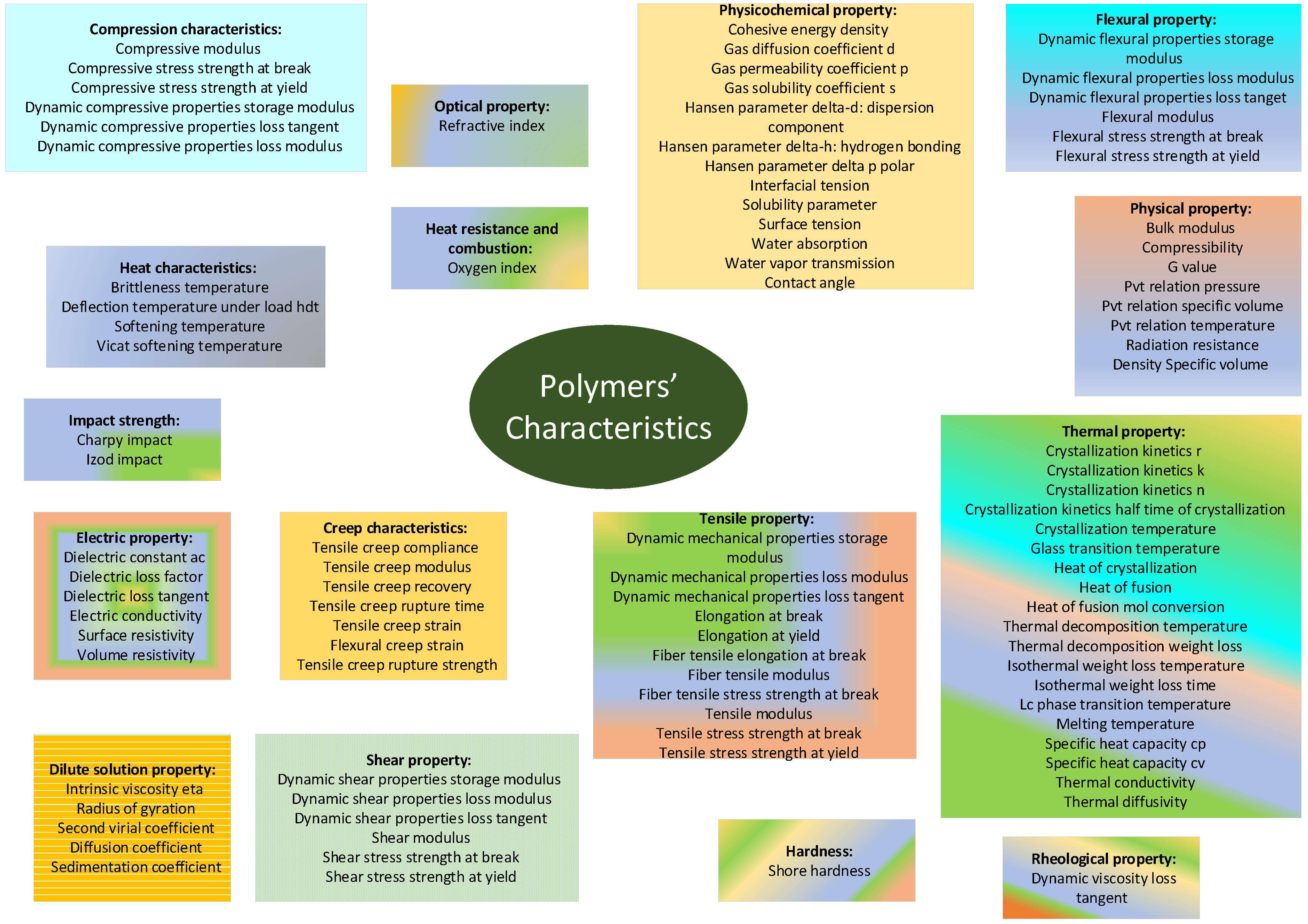
2.5. Categories of Characteristics
3. Results
4. Discussion
- Colloids: different models may be suitable for predicting properties such as particle size, shape, and stability, considering the diverse interactions and conditions influencing colloidal systems [65].
- Nucleic Acids: the unique properties of nucleic acids, such as DNA or RNA, may demand different models for predicting structural features [68], interaction energies, or other physical descriptors based on the specific characteristics of the dataset.
5. Conclusions
- 1.
- Feature Engineering and Selection: explore advanced feature engineering techniques and refine feature selection methods to identify the most influential characteristics. Investigate the impact of incorporating domain-specific knowledge to enhance the models’ ability to capture subtle nuances in polymer behavior.
- 2.
- Model Optimization: this includes experimenting with different ensemble methods, regularization techniques, and model architectures to achieve a more robust and accurate predictive framework.
- 3.
- Dataset Expansion: consider augmenting the dataset by incorporating data from diverse polymer sources. A larger and more diverse dataset could provide a comprehensive understanding of polymer characteristics, enabling models to generalize better across different types of polymers.
- 4.
- Cross-Dataset Validation: evaluate the transferability of the developed models by validating them on external polymer datasets. Assessing the models’ performance on different datasets will provide insights into their robustness and applicability across various polymer compositions and properties.
- 5.
- Incorporating Temporal Aspects: if applicable, consider incorporating temporal aspects into the models to capture any time-dependent trends or changes in polymer characteristics. This could involve analyzing how polymers evolve over time under different conditions.
- 6.
- Interpretability and Explainability: enhance the interpretability of the models to provide clearer insights into the features driving predictions. This could involve employing techniques such as SHAP (SHapley Additive exPlanations) values to explain the contribution of each feature to the model’s output.
- 7.
- Uncertainty Quantification: integrate methods for uncertainty quantification to provide more reliable predictions and confidence intervals. This is particularly important in applications where understanding the uncertainty associated with predictions is crucial for decision-making.
- 8.
- Collaboration with Domain Experts: foster collaboration between data scientists and domain experts in polymer science to gain deeper insights into the underlying physics and chemistry. Leveraging domain knowledge can lead to the development of more informed models and a better understanding of the relationships between polymer characteristics.
Author Contributions
Funding
Institutional Review Board Statement
Data Availability Statement
Conflicts of Interest
Appendix A. Data Description

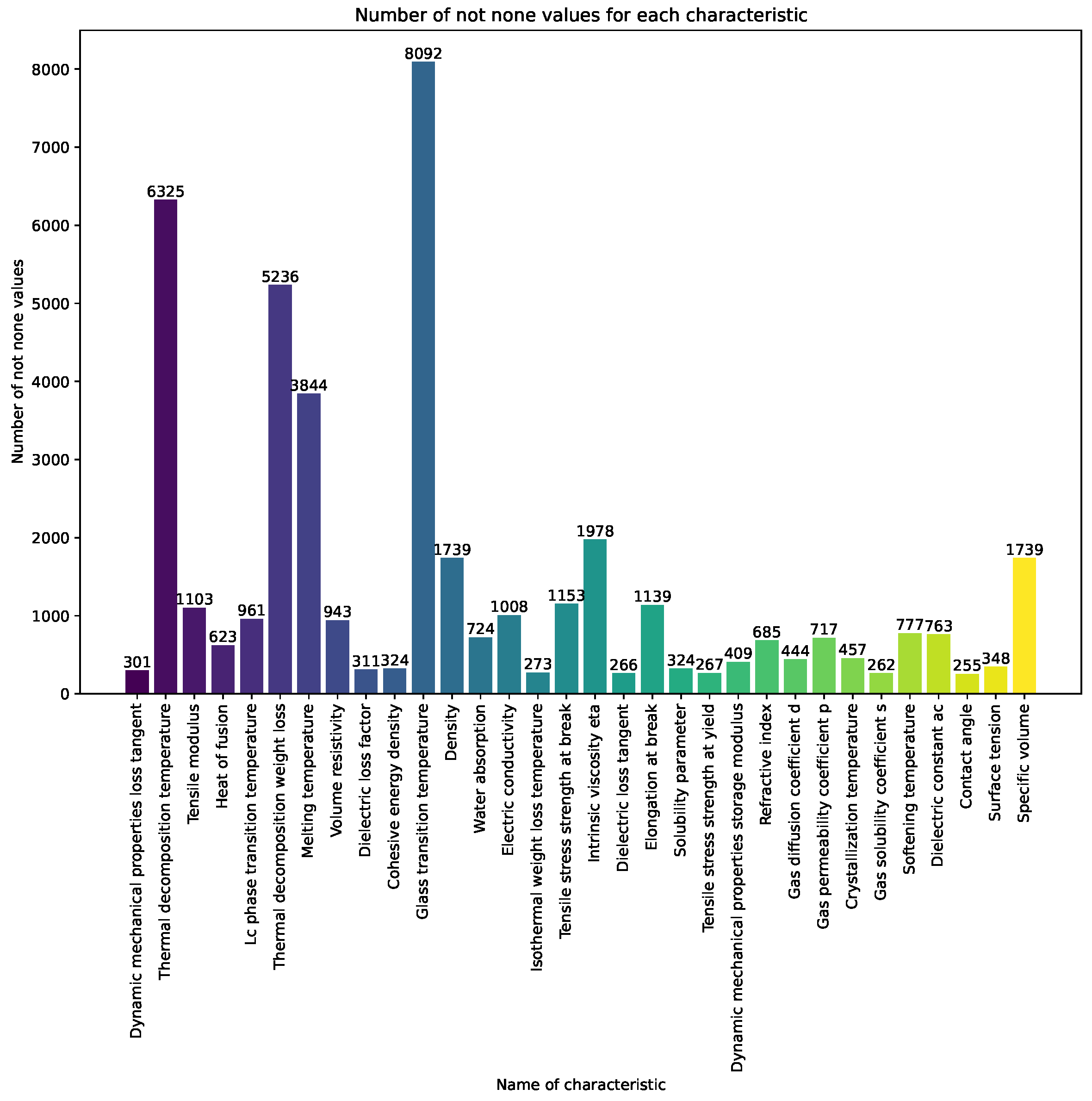
| Characteristic | Count | Mean | Std | Min | Max | 50% | Unit |
|---|---|---|---|---|---|---|---|
| Dynamic mechanical properties loss tangent | 301 | 0.56 | 1.12 | 0.0 | 11.6 | 0.14 | |
| Thermal decomposition temperature | 6325 | 401.0 | 112.87 | 18.0 | 1000.0 | 403.0 | C |
| Tensile modulus | 1103 | 3.69 | 13.03 | 0.0 | 202.0 | 2.1 | GPa |
| Heat of fusion | 623 | 0.01 | 0.01 | 0.0 | 0.12 | 0.01 | kcal/g |
| LC phase transition temperature | 961 | 191.76 | 95.37 | −90.0 | 528.0 | 175.0 | C |
| Thermal decomposition weight loss | 5236 | 10.25 | 13.09 | 0.0 | 100.0 | 5.0 | % |
| Melting temperature | 3844 | 194.93 | 108.24 | −54.0 | 580.0 | 186.35 | C |
| Volume resistivity | 943 | 0.0 | ohm·cm | ||||
| Dielectric loss factor | 311 | 775.51 | 13608.97 | 0.0 | 240000.0 | 0.1 | |
| Cohesive energy density | 324 | 112.21 | 60.3 | 0.0 | 626.0 | 96.0 | cal/cm3 |
| Glass transition temperature | 8092 | 145.18 | 110.69 | −123.0 | 495.0 | 138.0 | C |
| Density | 1739 | 1.24 | 0.2 | 0.23 | 3.03 | 1.23 | g/cm3 |
| Water absorption | 724 | 10.95 | 48.98 | 0.0 | 1065.0 | 2.5 | wt% |
| Electric conductivity | 1008 | 0.0 | 0.0 | 1/(ohm·cm) | |||
| Elongation at break | 1139 | 51.98 | 157.26 | 0.26 | 3000.0 | 10.1 | % |
| Tensile stress strength at break | 1153 | 0.19 | 2.14 | 0.0 | 64.02 | 0.08 | GPa |
| Intrinsic viscosity ETA | 1978 | 1.43 | 12.4 | 0.0 | 495.0 | 0.52 | dl/g |
| Solubility parameter | 324 | 21.08 | 5.0 | 0.0 | 51.2 | 20.0 | (J/cm3) |
| Dynamic mechanical properties storage modulus | 409 | 2.28 | 4.58 | 0.0 | 64.6 | 1.3 | GPa |
| Refractive index | 685 | 1.65 | 0.86 | 0.49 | 23.0 | 1.6 | |
| Gas diffusion coefficient d | 444 | 0.0 | 0.0 | 0.0 | 0.0 | 0.0 | cm2/s |
| Gas permeability coefficient p | 717 | 0.0 | 0.0 | 0.0 | 0.0 | 0.0 | cm3(STP)cm/(cm2·s·Pa) |
| Crystallization temperature | 457 | 138.4 | 105.61 | −120.0 | 496.0 | 124.0 | C |
| Softening temperature | 777 | 176.31 | 103.88 | −185.0 | 800.0 | 173.0 | C |
| Dielectric constant AC | 763 | 22.51 | 403.72 | 0.12 | 11,002.15 | 3.26 | |
| Surface tension | 348 | 30.95 | 13.08 | 5.75 | 72.5 | 31.13 | mN/m |
| Specific volume | 1739 | 0.83 | 0.15 | 0.33 | 4.3 | 0.81 | cm3/g |
| Dielectric loss tangent | 266.0 | 0.74 | 4.8 | −0.03 | 55.0 | 0.02 | |
| Isothermal weight loss temperature | 273.0 | 389.35 | 165.13 | 100.0 | 900.0 | 350.0 | C |
| Tensile stress strength at yield | 267.0 | 0.07 | 0.05 | 0.0 | 0.4 | 0.06 | GPa |
| Contact angle | 255.0 | 73.96 | 19.85 | 15.0 | 158.9 | 76.0 | degree |
| Gas solubility coefficient s | 262.0 | 0.01 | 0.06 | 0.0 | 0.69 | 0.0 | cm3 (STP)/cm3·Pa) |
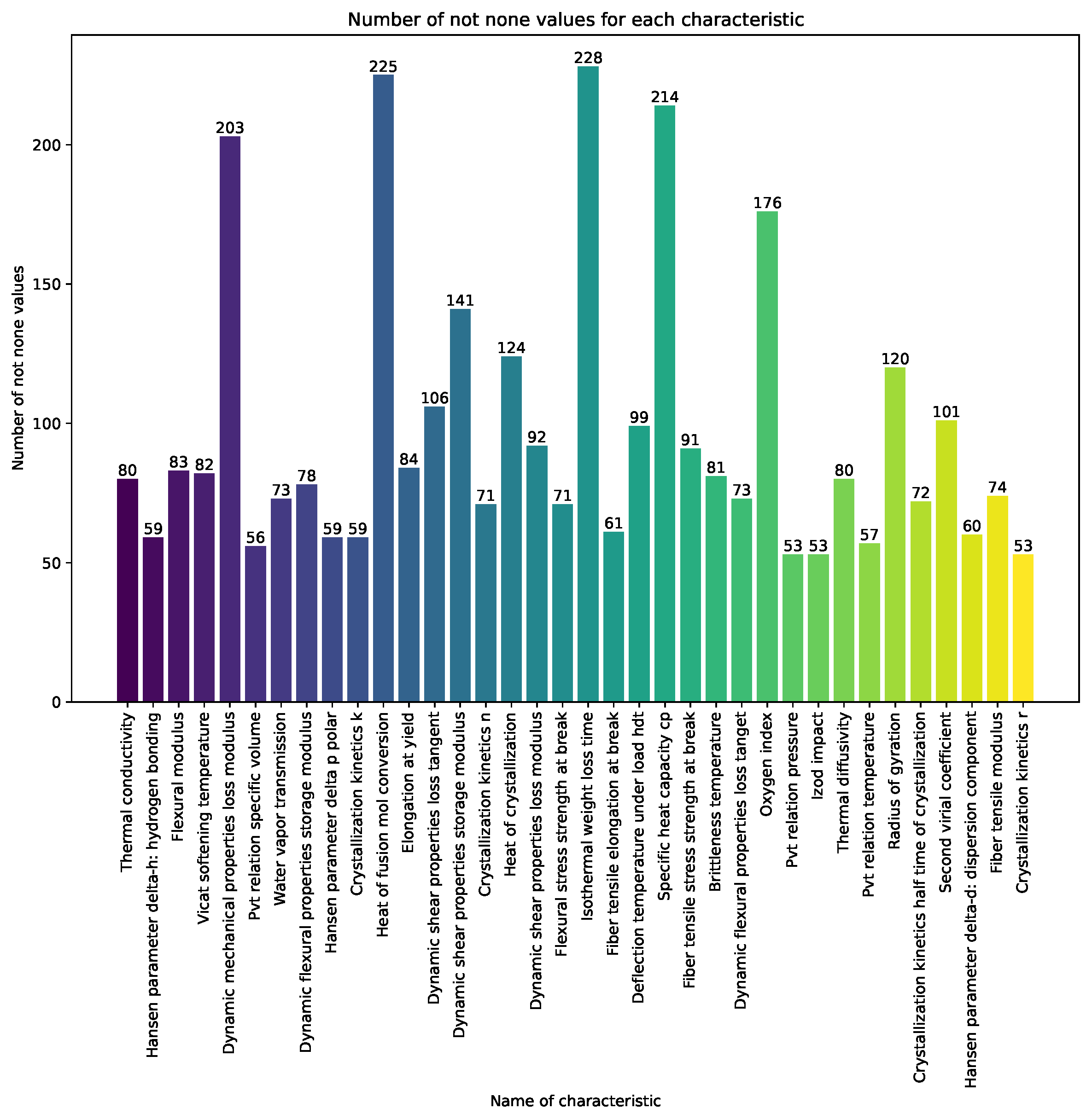
| Characteristic | Count | Mean | Std | Min | Max | 50% | Unit |
|---|---|---|---|---|---|---|---|
| Thermal conductivity | 80 | 0.81 | 2.95 | 0.01 | 23.0 | 0.22 | W/(m·K) |
| Hansen parameter delta−h: hydrogen bonding | 59 | 8.03 | 3.5 | 0.0 | 16.0 | 7.4 | (J/cm |
| Flexural modulus | 83 | 8.27 | 21.18 | 0.04 | 108.0 | 2.61 | GPa |
| Vicat softening temperature | 82 | 137.08 | 59.47 | 29.7 | 380.0 | 133.0 | C |
| Dynamic mechanical properties loss modulus | 203 | 2.47 | 22.2 | 0.0 | 260.0 | 0.1 | GPa |
| PVT relation specific volume | 56 | 0.85 | 0.17 | 0.4 | 1.17 | 0.85 | cmcm3/g |
| Water vapor transmission | 73 | 0.82 | 2.38 | 0.0 | 15.0 | 0.01 | g·mil/(cm2·24 h) |
| Dynamic flexural properties storage modulus | 78 | 1.71 | 4.36 | 0.0 | 37.0 | 0.79 | GPa |
| Hansen parameter delta p polar | 59 | 7.11 | 4.84 | 1.1 | 19.5 | 6.1 | (J/cm |
| Crystallization kinetics k | 59 | 0.66 | 2.25 | 0.0 | 15.07 | 0.01 | |
| Heat of fusion mol conversion | 225 | 3.99 | 3.33 | 0.0 | 21.0 | 3.32 | kcal/mol |
| Elongation at yield | 84 | 22.45 | 50.18 | 0.08 | 334.0 | 8.3 | % |
| Dynamic shear properties loss tangent | 106 | 1.88 | 14.6 | 0.0 | 150.0 | 0.07 | |
| Dynamic shear properties storage modulus | 141 | 0.43 | 0.67 | 0.0 | 3.65 | 0.03 | GPa |
| Crystallization kinetics n | 71 | 2.59 | 0.72 | 0.59 | 4.15 | 2.6 | |
| Heat of crystallization | 124.0 | 10.39 | 9.95 | 0.29 | 49.3 | 8.3 | cal/g |
| Dynamic shear properties loss modulus | 92 | 0.05 | 0.11 | 0.0 | 0.7 | 0.0 | GPa |
| Flexural stress strength at break | 71 | 0.15 | 0.29 | 0.0 | 1.84 | 0.09 | GPa |
| Isothermal weight loss time | 228 | 86.9 | 333.57 | 0.18 | 2500.0 | 13.8 | h |
| Fiber tensile elongation at break | 61 | 39.65 | 48.71 | 2.25 | 242.34 | 21.0 | % |
| Deflection temperature under load HDT | 99 | 189.38 | 87.48 | 45.0 | 417.0 | 197.0 | C |
| Specific heat capacity CP | 214 | 0.38 | 0.25 | 0.0 | 2.52 | 0.35 | cal/(g·C) |
| Fiber tensile stress strength at break | 91 | 50.8 | 329.54 | 0.17 | 3090.0 | 3.6 | g/denier |
| Brittleness temperature | 81 | −22.15 | 35.05 | −80.0 | 90.0 | −26.0 | C |
| Dynamic flexural properties loss tanget | 73 | 0.59 | 0.71 | 0.0 | 3.02 | 0.17 | |
| Oxygen index | 176 | 35.85 | 14.05 | 4.5 | 95.0 | 34.0 | % |
| PVT relation pressure | 53 | 74.91 | 135.54 | 0.0 | 598.8 | 35.0 | MPa |
| Izod impact | 53 | 161.43 | 350.27 | 0.02 | 1990.0 | 40.0 | kJ/m |
| Thermal diffusivity | 80 | 0.0 | 0.0 | 0.0 | 0.0 | 0.0 | m2/s |
| PVT relation temperature | 57 | 216.95 | 523.81 | 4.0 | 3822.0 | 87.5 | C |
| Radius of gyration | 120 | 33.15 | 36.39 | 0.5 | 264.35 | 21.72 | nm |
| Crystallization kinetics half time of crystallization | 72 | 2389.53 | 6064.79 | 11.1 | 35,400.0 | 289.5 | s |
| Second virial coefficient | 101 | 0.15 | 1.07 | −0.0 | 8.95 | 0.0 | cm3·mol/g2 |
| Hansen parameter delta−d: dispersion component | 60 | 16.54 | 4.09 | 0.0 | 21.5 | 17.53 | (J/cm |
| Fiber tensile modulus | 74 | 90.59 | 156.26 | 3.86 | 847.0 | 43.5 | g/denier |
| Crystallization kinetics r | 53 | 1986.31 | 10,850.65 | 0.02 | 79,175.0 | 97.0 | nm/s |
Appendix B. Physical Characteristics
Appendix B.1. Physical Properties
- 1.
- Bulk Modulus: measures a material’s resistance to volume change under pressure. It is crucial for understanding how a material responds to changes in pressure [69].
- 2.
- Compressibility: describes the degree to which a material can be compressed. It is the reciprocal of bulk modulus and helps assess a material’s response to external pressure [70].
- 3.
- G Value: represents the ratio of the strain energy stored in a material to the kinetic energy. It provides insights into a material’s elastic behavior under deformation [71].
- 4.
- PVT Relation Pressure: describes the relationship between pressure and specific volume in a material. It is essential for understanding the material’s response to changes in pressure and volume [72].
- 5.
- PVT Relation Specific Volume: defines the correlation between specific volume and pressure in a material. It is crucial for analyzing the material’s behavior under varying pressure conditions [73].
- 6.
- PVT Relation Temperature: illustrates the relationship between temperature and specific volume in a material. It is essential for studying how temperature influences the material’s volume properties [74].
- 7.
- Radiation Resistance: measures a material’s ability to withstand the effects of ionizing radiation. This property is vital for materials used in radiation-exposed environments [75].
- 8.
- Density: represents the mass of a material per unit volume. Density is a fundamental property that influences various material characteristics [76].
- 9.
- Specific Volume: describes the volume occupied by a unit mass of a material. It is the reciprocal of density and provides insights into material compactness [77].
Appendix B.2. Compression Characteristics
- 1.
- Compressive Modulus: measures the material’s resistance to compression. Essential in the construction of structural elements made of polymers [78].
- 2.
- Compressive Stress Strength at Break: determines the maximum pressure a polymer can withstand before breaking. Important for assessing the resilience of polymer structures to mechanical forces [79].
- 3.
- Compressive Stress Strength at Yield: measures the strength of a polymer under pressure before plastic deformation begins. Important for the preliminary evaluation of the material’s structural reliability [80].
- 4.
- Dynamic Compressive Properties Storage Modulus: characterizes the material’s ability to store energy under dynamic loading. Important for materials subjected to cyclic loads, such as in damping materials [81].
- 5.
- Dynamic Compressive Properties Loss Tangent: reflects the fraction of energy loss due to dynamic deformation. Important in the development of materials with effective damping properties [82].
- 6.
- Dynamic Compressive Properties Loss Modulus: determines the energy loss during dynamic deformation. Important for materials designed for sound absorption or vibration reduction [83].
Appendix B.3. Creep Characteristics
- 1.
- Tensile Creep Compliance: determines the polymer’s ability to undergo deformation under constant tensile load. This is crucial for assessing the long-term stability of polymer materials under constant force or load [84].
- 2.
- Tensile Creep Modulus: measures the elasticity of the polymer when deformed under constant force. This parameter is useful in designing materials for applications where resistance to constant mechanical loads is important [85].
- 3.
- Tensile Creep Recovery: evaluates the polymer’s ability to return to its original shape after deformation under tensile loading. This is important, for example, for materials used in springs or elastic elements [86].
- 4.
- Tensile Creep Rupture Time: specifies the period during which the polymer undergoes deformation before rupture under tensile loading. This is an important characteristic for assessing the material’s resistance to long-term mechanical loads [87].
- 5.
- Tensile Creep Strain: measures the level of deformation a polymer can undergo under constant tensile force. This is important for understanding the material’s behavior under constant load and can be used in the design of structural elements [88].
- 6.
- Flexural Creep Strain: evaluates the deformation of the polymer under constant load during bending. This characteristic is important, for example, when using polymer materials in structures subjected to constant bending forces [89].
- 7.
- Tensile Creep Rupture Strength: determines the maximum load a polymer can withstand before rupture under constant tensile force. This is a crucial parameter for assessing the durability and resilience of polymer materials under constant mechanical loads [90].
Appendix B.4. Dilute Solution Property
- 1.
- Intrinsic Viscosity (): measures the polymer’s resistance to flow in a dilute solution, providing insights into its molecular size and structure. Intrinsic viscosity is crucial for understanding the polymer’s solubility and processing behavior [91].
- 2.
- Radius of Gyration: defines the average distance of polymer segments from the center of mass, indicating the spatial extent of the polymer chain in solution. This property is significant in studying polymer conformations [92].
- 3.
- Second Virial Coefficient: describes the non-ideality of polymer solutions, providing information about the intermolecular interactions and solute-solvent interactions. This coefficient influences the solution behavior and phase separation [93].
- 4.
- Diffusion Coefficient: represents the rate at which polymer molecules spread through the solution, influencing mass transport and the polymer’s ability to interact with its surroundings [94].
- 5.
- Sedimentation Coefficient: measures the rate at which polymer particles settle under the influence of gravity in a centrifugal field, providing information about particle size and shape in solution [95].
Appendix B.5. Electric Property
- 1.
- Dielectric Constant (AC): reflects the material’s ability to store electrical energy in an alternating current (ac) field. The dielectric constant influences the capacitance of electronic components [96].
- 2.
- Dielectric Loss Factor: measures the efficiency with which a dielectric material converts electrical energy into heat. This property is crucial in applications where minimal energy loss is desired [97].
- 3.
- Dielectric Loss Tangent: describes the ratio of the dielectric loss factor to the dielectric constant, providing insights into the material’s efficiency in handling electrical energy [98].
- 4.
- Electric Conductivity: represents the ability of a material to conduct electric current. This property is essential in various electronic and electrical applications [99].
- 5.
- Surface Resistivity: defines the electrical resistance across the surface of a material, influencing its performance in applications where surface conductivity is critical [100].
- 6.
- Volume Resistivity: measures the electrical resistance through the volume of a material, providing information about its overall resistance to electric current flow [101].
Appendix B.6. Flexural Property
- 1.
- Dynamic Flexural Properties Storage Modulus: characterizes the material’s ability to store energy under dynamic flexural (bending) loading conditions. Important for materials subjected to cyclic loads [102].
- 2.
- Dynamic Flexural Properties Loss Modulus: determines the energy dissipation capacity of the material during dynamic flexural deformation. Relevant for applications requiring effective damping [103].
- 3.
- Dynamic Flexural Properties Loss Tangent: reflects the ratio of the loss modulus to the storage modulus in dynamic flexural deformation, providing insights into the material’s damping behavior [104].
- 4.
- Flexural Modulus: measures the material’s stiffness and resistance to bending deformation. Crucial in designing structural components where flexural strength is essential [105].
- 5.
- Flexural Stress Strength at Break: indicates the maximum stress a material can withstand before fracturing under bending stress. Important for evaluating the material’s structural integrity [106].
- 6.
- Flexural Stress Strength at Yield: measures the material’s stress resistance under bending before exhibiting plastic deformation. Important for assessing structural reliability under flexural loads [107].
Appendix B.7. Hardness
- 1.
- Shore Hardness: measures the resistance of the material to indentation or penetration. Shore hardness is a valuable indicator of a material’s overall hardness and durability [108].
Appendix B.8. Heat Characteristics
- 1.
- Brittleness Temperature: indicates the temperature at which a material transitions from a flexible to a brittle state, providing insight into its low-temperature performance [109].
- 2.
- Deflection Temperature under Load (HDT): represents the temperature at which a standard test bar experiences a specified deformation under a specific load. HDT is crucial for understanding a material’s ability to withstand elevated temperatures while supporting a load [110].
- 3.
- Softening Temperature: defines the temperature range at which a material starts to soften, losing its rigidity. Softening temperature is essential for assessing a material’s behavior under heat [111].
- 4.
- Vicat Softening Temperature: determines the temperature at which a needle penetrates a material under a specified load. Vicat softening temperature provides insights into the heat resistance and stability of a material [112].
Appendix B.9. Heat Resistance and Combustion
- 1.
- Oxygen Index: measures the minimum concentration of oxygen in a mixture with an inert gas that supports the combustion of a material. This parameter is crucial for evaluating a material’s fire resistance and combustion characteristics [113].
Appendix B.10. Impact Strength
- 1.
- Charpy Impact: assesses a material’s resistance to sudden impact by measuring the amount of energy absorbed during fracture. Charpy impact testing is widely used to evaluate the toughness of materials [114].
- 2.
- Izod Impact: similar to Charpy impact testing, Izod impact testing measures a material’s resistance to impact. It assesses the energy required to break a notched specimen under a sudden impact [115].
Appendix B.11. Optical Property
- 1.
- Refractive Index: determines the degree to which light is refracted or bent as it passes through a material. Refractive index is essential for understanding optical transparency and performance in various applications [116].
Appendix B.12. Physicochemical Property
- 1.
- Cohesive Energy Density: represents the energy required to separate unit volumes of material. It is a measure of the cohesive forces within a substance [117].
- 2.
- Gas Diffusion Coefficient (D): describes the rate at which gas molecules diffuse through a substance. It is crucial for understanding gas transport properties [118].
- 3.
- Gas Permeability Coefficient (P): measures a material’s ability to allow gas permeation. It is essential for applications where gas barrier properties are significant [119].
- 4.
- Gas Solubility Coefficient (S): represents the capacity of a material to dissolve gases. This property is vital for understanding gas absorption in polymers [120].
- 5.
- Hansen Parameter : Dispersion Component: describes the dispersion forces within a material. It is part of the Hansen solubility parameters, which characterize solute-solvent interactions [121].
- 6.
- Hansen Parameter : Hydrogen Bonding: represents the hydrogen bonding contribution to the Hansen solubility parameters. It provides insights into materials’ compatibility with various solvents [122].
- 7.
- Hansen Parameter : Polar: describes the polar forces within a material. It is another component of the Hansen solubility parameters [123].
- 8.
- Interfacial Tension: measures the energy required to increase the surface area between two phases. It is crucial for understanding interactions at material interfaces [124].
- 9.
- Solubility Parameter: represents the overall solubility characteristics of a substance. It is a combination of the Hansen parameters and is used to predict material compatibility [125].
- 10.
- Surface Tension: describes the force acting on the surface of a liquid that tends to minimize the area. Surface tension is vital for understanding wetting and adhesion [126].
- 11.
- Water Absorption: measures the ability of a material to absorb water. It is essential for assessing the material’s response to humid environments [127].
- 12.
- Water Vapor Transmission: describes the rate at which water vapor permeates through a material. It is crucial for applications requiring water vapor barrier properties [128].
- 13.
- Contact Angle: represents the angle formed between a liquid droplet and a solid surface. It provides insights into the wettability of a material [129].
Appendix B.13. Rheological Property
- 1.
- Dynamic Viscosity Loss Tangent: describes the ratio of the loss modulus to the storage modulus in the context of dynamic viscosity. It provides insights into the energy dissipation behavior of the material under dynamic conditions [130].
Appendix B.14. Shear Property
- 1.
- Dynamic Shear Properties Storage Modulus: represents the ability of a material to store elastic energy under shear stress in dynamic conditions [131].
- 2.
- Dynamic Shear Properties Loss Modulus: describes the portion of energy that a material loses as heat under shear stress in dynamic conditions [132].
- 3.
- Dynamic Shear Properties Loss Tangent: represents the ratio of the loss modulus to the storage modulus in the context of dynamic shear properties. It provides insights into the material’s response to shear forces [133].
- 4.
- Shear Modulus: measures a material’s resistance to deformation under shear stress. It is crucial for understanding a material’s shear behavior [134].
- 5.
- Shear Stress Strength at Break: represents the maximum shear stress a material can withstand before experiencing failure. It is an essential parameter for evaluating the material’s shear strength [135].
- 6.
- Shear Stress Strength at Yield: measures the shear stress a material can withstand before undergoing plastic deformation. This parameter is crucial for assessing the material’s yield strength under shear forces [136].
Appendix B.15. Tensile Property
- 1.
- Dynamic Mechanical Properties Storage Modulus: represents the material’s ability to store elastic energy under dynamic tensile conditions [137].
- 2.
- Dynamic Mechanical Properties Loss Modulus: describes the portion of energy that a material loses as heat under dynamic tensile conditions [138].
- 3.
- Dynamic Mechanical Properties Loss Tangent: represents the ratio of the loss modulus to the storage modulus in the context of dynamic tensile properties. It provides insights into the material’s response to dynamic tensile forces [139].
- 4.
- Elongation at Break: measures the extent to which a material can stretch before experiencing rupture. It is a crucial parameter for evaluating the material’s ductility [140].
- 5.
- Elongation at Yield: measures the material’s deformation before it starts yielding under tensile stress. This parameter provides insights into the material’s yield behavior under tension [141].
- 6.
- Fiber Tensile Elongation at Break: describes the elongation capability of fiber materials before experiencing rupture under tensile stress [142].
- 7.
- Fiber Tensile Modulus: represents the stiffness of a fiber material under tensile stress. It is a critical parameter for assessing the material’s tensile rigidity [143].
- 8.
- Fiber Tensile Stress Strength at Break: represents the maximum tensile stress a fiber material can withstand before undergoing rupture [144].
- 9.
- Tensile Modulus: measures the material’s resistance to deformation under tensile stress. It is crucial for understanding the material’s tensile behavior [145].
- 10.
- Tensile Stress Strength at Break: represents the maximum tensile stress a material can withstand before experiencing failure [146].
- 11.
- Tensile Stress Strength at Yield: measures the tensile stress a material can withstand before undergoing plastic deformation. This parameter is crucial for assessing the material’s yield strength under tensile forces [147].
Appendix B.16. Thermal Property
- 1.
- Crystallization Kinetics r: characterizes the crystallization kinetics of a material, representing the rate of crystallization [148].
- 2.
- Crystallization Kinetics k: represents a parameter in the crystallization kinetics equation, providing insights into the crystallization process [149].
- 3.
- Crystallization Kinetics n: another parameter in the crystallization kinetics equation, influencing the rate of crystallization [150].
- 4.
- Crystallization Kinetics Half Time of Crystallization: describes the time required for half of the crystallization process to occur [151].
- 5.
- Crystallization Temperature: represents the temperature at which a material undergoes crystallization [152].
- 6.
- Glass Transition Temperature: indicates the temperature at which an amorphous material transitions from a rigid to a rubbery state [153].
- 7.
- Heat of Crystallization: represents the amount of heat released or absorbed during the crystallization process [154].
- 8.
- Heat of Fusion: describes the heat energy required to change a substance from a solid to a liquid state at a constant temperature [155].
- 9.
- Heat of Fusion Mol Conversion: provides insights into the heat energy required for the conversion of a mole of substance from solid to liquid state [156].
- 10.
- Thermal Decomposition Temperature: represents the temperature at which a material starts to decompose thermally [157].
- 11.
- Thermal Decomposition Weight Loss: describes the weight loss associated with the thermal decomposition of a material [158].
- 12.
- Isothermal Weight Loss Temperature: represents the temperature maintained during a process where a material experiences weight loss [159].
- 13.
- Isothermal Weight Loss Time: describes the duration of time during which a material undergoes weight loss under isothermal conditions [160].
- 14.
- LC Phase Transition Temperature: represents the temperature at which a phase transition occurs in the liquid crystalline state [161].
- 15.
- Melting Temperature: indicates the temperature at which a material transitions from a solid to a liquid state [162].
- 16.
- Specific Heat Capacity : describes the amount of heat energy required to raise the temperature of a unit mass of a material by one degree Celsius at constant pressure [163].
- 17.
- Specific Heat Capacity : similar to but at constant volume, representing the heat energy required to raise the temperature at constant volume [164].
- 18.
- Thermal Conductivity: describes the ability of a material to conduct heat [165].
- 19.
- Thermal Diffusivity: represents the ability of a material to conduct heat relative to its ability to store heat. It is the ratio of thermal conductivity to volumetric heat capacity [166].
References
- Bates, F.S. Polymer-polymer phase behavior. Science 1991, 251, 898–905. [Google Scholar] [CrossRef]
- Jenkins, A.D. Polymer Science: A Materials Science Handbook; Elsevier: Amsterdam, The Netherlands, 2013. [Google Scholar]
- Ligon, S.C.; Liska, R.; Stampfl, J.; Gurr, M.; Mulhaupt, R. Polymers for 3D printing and customized additive manufacturing. Chem. Rev. 2017, 117, 10212–10290. [Google Scholar] [CrossRef]
- Aidoo, R.P.; Depypere, F.; Afoakwa, E.O.; Dewettinck, K. Industrial manufacture of sugar-free chocolates–Applicability of alternative sweeteners and carbohydrate polymers as raw materials in product development. Trends Food Sci. Technol. 2013, 32, 84–96. [Google Scholar] [CrossRef]
- Li, V.C. Tailoring ECC for special attributes: A review. Int. J. Concr. Struct. Mater. 2012, 6, 135–144. [Google Scholar] [CrossRef]
- Kesarwani, S. Polymer composites in aviation sector. Int. J. Eng. Res 2017, 6, 10. [Google Scholar] [CrossRef]
- Jenkins, M.; Stamboulis, A. Durability and Reliability of Medical Polymers; Elsevier: Amsterdam, The Netherlands, 2012. [Google Scholar]
- Hong, Y.; Cooper-White, J.; Mackay, M.; Hawker, C.; Malmström, E.; Rehnberg, N. A novel processing aid for polymer extrusion: Rheology and processing of polyethylene and hyperbranched polymer blends. J. Rheol. 1999, 43, 781–793. [Google Scholar] [CrossRef]
- Ohshima, M.; Tanigaki, M. Quality control of polymer production processes. J. Process Control 2000, 10, 135–148. [Google Scholar] [CrossRef]
- Stevenson, S.; Vaisey-Genser, M.; Eskin, N. Quality control in the use of deep frying oils. J. Am. Oil Chem. Soc. 1984, 61, 1102–1108. [Google Scholar] [CrossRef]
- Del Nobile, M.A.; Conte, A.; Buonocore, G.G.; Incoronato, A.; Massaro, A.; Panza, O. Active packaging by extrusion processing of recyclable and biodegradable polymers. J. Food Eng. 2009, 93, 1–6. [Google Scholar] [CrossRef]
- Borgquist, P.; Körner, A.; Piculell, L.; Larsson, A.; Axelsson, A. A model for the drug release from a polymer matrix tablet—effects of swelling and dissolution. J. Control. Release 2006, 113, 216–225. [Google Scholar] [CrossRef]
- Ranstam, J.; Cook, J. LASSO regression. J. Br. Surg. 2018, 105, 1348. [Google Scholar] [CrossRef]
- De Mol, C.; De Vito, E.; Rosasco, L. Elastic-net regularization in learning theory. J. Complex. 2009, 25, 201–230. [Google Scholar] [CrossRef]
- Xu, M.; Watanachaturaporn, P.; Varshney, P.K.; Arora, M.K. Decision tree regression for soft classification of remote sensing data. Remote Sens. Environ. 2005, 97, 322–336. [Google Scholar] [CrossRef]
- Breiman, L. Bagging predictors. Mach. Learn. 1996, 24, 123–140. [Google Scholar] [CrossRef]
- Solomatine, D.P.; Shrestha, D.L. AdaBoost. RT: A boosting algorithm for regression problems. In Proceedings of the 2004 IEEE International Joint Conference on Neural Networks, Budapest, Hungary, 25–29 July 2004; Volume 2, pp. 1163–1168. [Google Scholar]
- Zhang, X.; Yan, C.; Gao, C.; Malin, B.A.; Chen, Y. Predicting missing values in medical data via XGBoost regression. J. Healthc. Inform. Res. 2020, 4, 383–394. [Google Scholar] [CrossRef]
- Awad, M.; Khanna, R.; Awad, M.; Khanna, R. Support vector regression. Efficient Learning Machines: Theories, Concepts, and Applications for Engineers and System Designers; Springer: Berlin, Germany, 2015; pp. 67–80. [Google Scholar]
- Prettenhofer, P.; Louppe, G. Gradient boosted regression trees in scikit-learn. In Proceedings of the PyData 2014, London, UK, 21–23 February 2014. [Google Scholar]
- Weisberg, S. Applied Linear Regression; John Wiley & Sons: Hoboken, NJ, USA, 2005; Volume 528. [Google Scholar]
- Liu, Y.; Wang, Y.; Zhang, J. New machine learning algorithm: Random forest. In Proceedings of the Information Computing and Applications: Third International Conference, ICICA 2012, Chengde, China, 14–16 September 2012; pp. 246–252. [Google Scholar]
- Li, F.; Yang, Y.; Xing, E. From lasso regression to feature vector machine. Adv. Neural Inf. Process. Syst. 2005, 18, 18. [Google Scholar]
- James, G.M.; Wang, J.; Zhu, J. Functional linear regression that’s interpretable. Ann. Statist. 2009, 37, 2083–2108. [Google Scholar] [CrossRef]
- Mohammed Rashid, A.; Midi, H.; Dhhan, W.; Arasan, J. Detection of outliers in high-dimensional data using nu-support vector regression. J. Appl. Stat. 2022, 49, 2550–2569. [Google Scholar] [CrossRef]
- Segal, M.R. Machine learning benchmarks and random forest regression. J. Data Anal. Inf. Process. 2004, 8, 4. [Google Scholar]
- Koyamparambath, A.; Adibi, N.; Szablewski, C.; Adibi, S.A.; Sonnemann, G. Implementing artificial intelligence techniques to predict environmental impacts: Case of construction products. Sustainability 2022, 14, 3699. [Google Scholar] [CrossRef]
- Sancar, N.; Onakpojeruo, E.P.; Inan, D.; Ozsahin, D.U. Adaptive Elastic Net Based on Modified PSO for Variable Selection in Cox Model with High-dimensional Data: A Comprehensive Simulation Study. IEEE Access 2023, 11, 127302–127316. [Google Scholar] [CrossRef]
- Paez, A.; López, F.; Ruiz, M.; Camacho, M. Inducing non-orthogonal and non-linear decision boundaries in decision trees via interactive basis functions. Expert Syst. Appl. 2019, 122, 183–206. [Google Scholar] [CrossRef]
- Florez-Lopez, R.; Ramon-Jeronimo, J.M. Enhancing accuracy and interpretability of ensemble strategies in credit risk assessment. A correlated-adjusted decision forest proposal. Expert Syst. Appl. 2015, 42, 5737–5753. [Google Scholar] [CrossRef]
- Cao, J.; Kwong, S.; Wang, R. A noise-detection based AdaBoost algorithm for mislabeled data. Pattern Recognit. 2012, 45, 4451–4465. [Google Scholar] [CrossRef]
- Otchere, D.A.; Ganat, T.O.A.; Ojero, J.O.; Tackie-Otoo, B.N.; Taki, M.Y. Application of gradient boosting regression model for the evaluation of feature selection techniques in improving reservoir characterisation predictions. J. Pet. Sci. Eng. 2022, 208, 109244. [Google Scholar] [CrossRef]
- Ahmed, A.; Song, W.; Zhang, Y.; Haque, M.A.; Liu, X. Hybrid BO-XGBoost and BO-RF Models for the Strength Prediction of Self-Compacting Mortars with Parametric Analysis. Materials 2023, 16, 4366. [Google Scholar] [CrossRef]
- Wang, Z.; Bovik, A.C. Mean squared error: Love it or leave it? A new look at signal fidelity measures. IEEE Signal Process. Mag. 2009, 26, 98–117. [Google Scholar] [CrossRef]
- Miles, J. R-squared, adjusted R-squared. In Encyclopedia of Statistics in Behavioral Science; Wiley: Hoboken, NJ, USA, 2005. [Google Scholar]
- Chai, T.; Draxler, R.R. Root mean square error (RMSE) or mean absolute error (MAE)? Arguments against avoiding RMSE in the literature. Geosci. Model Dev. 2014, 7, 1247–1250. [Google Scholar] [CrossRef]
- Händel, P. Understanding normalized mean squared error in power amplifier linearization. IEEE Microw. Wirel. Components Lett. 2018, 28, 1047–1049. [Google Scholar] [CrossRef]
- Willmott, C.J.; Matsuura, K. Advantages of the mean absolute error (MAE) over the root mean square error (RMSE) in assessing average model performance. Clim. Res. 2005, 30, 79–82. [Google Scholar] [CrossRef]
- Jiang, Y. Estimation of monthly mean daily diffuse radiation in China. Appl. Energy 2009, 86, 1458–1464. [Google Scholar] [CrossRef]
- Polymer Database (PoLyInfo). Available online: https://polymer.nims.go.jp/ (accessed on 18 October 2023).
- Otsuka, S.; Kuwajima, I.; Hosoya, J.; Xu, Y.; Yamazaki, M. PoLyInfo: Polymer database for polymeric materials design. In Proceedings of the 2011 International Conference on Emerging Intelligent Data and Web Technologies, Tirana, Albania, 7–9 September 2011; pp. 22–29. [Google Scholar]
- Weininger, D. SMILES, a chemical language and information system. 1. Introduction to methodology and encoding rules. J. Chem. Inf. Comput. Sci. 1988, 28, 31–36. [Google Scholar] [CrossRef]
- Landrum, G. RDKit: A software suite for cheminformatics, computational chemistry, and predictive modeling. Greg Landrum 2013, 8, 31. [Google Scholar]
- Yang, L.; Shami, A. On hyperparameter optimization of machine learning algorithms: Theory and practice. Neurocomputing 2020, 415, 295–316. [Google Scholar] [CrossRef]
- Moons, K.G.; Donders, R.A.; Stijnen, T.; Harrell Jr, F.E. Using the outcome for imputation of missing predictor values was preferred. J. Clin. Epidemiol. 2006, 59, 1092–1101. [Google Scholar] [CrossRef] [PubMed]
- Charles, J.; Jassi, P.; Ananth, N.S.; Sadat, A.; Fedorova, A. Evaluation of the intel® core™ i7 turbo boost feature. In Proceedings of the 2009 IEEE International Symposium on Workload Characterization (IISWC), Austin, TX, USA, 4–6 October 2009; pp. 188–197. [Google Scholar]
- Lookman, T.; Alexander, F.J.; Rajan, K. Information Science for Materials Discovery and Design; Springer: Berlin, Germany, 2016; Volume 225. [Google Scholar]
- Mannodi-Kanakkithodi, A.; Chandrasekaran, A.; Kim, C.; Huan, T.D.; Pilania, G.; Botu, V.; Ramprasad, R. Scoping the polymer genome: A roadmap for rational polymer dielectrics design and beyond. Mater. Today 2018, 21, 785–796. [Google Scholar] [CrossRef]
- Doan Tran, H.; Kim, C.; Chen, L.; Chandrasekaran, A.; Batra, R.; Venkatram, S.; Kamal, D.; Lightstone, J.P.; Gurnani, R.; Shetty, P.; et al. Machine-learning predictions of polymer properties with Polymer Genome. J. Appl. Phys. 2020, 128, 10. [Google Scholar] [CrossRef]
- Kim, C.; Chandrasekaran, A.; Huan, T.D.; Das, D.; Ramprasad, R. Polymer genome: A data-powered polymer informatics platform for property predictions. J. Phys. Chem. C 2018, 122, 17575–17585. [Google Scholar] [CrossRef]
- Kazemi-Khasragh, E.; Blázquez, J.P.F.; Gómez, D.G.; González, C.; Haranczyk, M. Facilitating polymer property prediction with machine learning and group interaction modelling methods. Int. J. Solids Struct. 2024, 286, 112547. [Google Scholar] [CrossRef]
- Antoniuk, E.R.; Li, P.; Kailkhura, B.; Hiszpanski, A.M. Representing Polymers as Periodic Graphs with Learned Descriptors for Accurate Polymer Property Predictions. J. Chem. Inf. Model. 2022, 62, 5435–5445. [Google Scholar] [CrossRef]
- Xie, T.; Grossman, J.C. Crystal graph convolutional neural networks for an accurate and interpretable prediction of material properties. Phys. Rev. Lett. 2018, 120, 145301. [Google Scholar] [CrossRef]
- Yang, K.; Swanson, K.; Jin, W.; Coley, C.; Eiden, P.; Gao, H.; Guzman-Perez, A.; Hopper, T.; Kelley, B.; Mathea, M.; et al. Analyzing learned molecular representations for property prediction. J. Chem. Inf. Model. 2019, 59, 3370–3388. [Google Scholar] [CrossRef] [PubMed]
- Schindler, P.; Antoniuk, E.R.; Cheon, G.; Zhu, Y.; Reed, E.J. Discovery of materials with extreme work functions by high-throughput density functional theory and machine learning. arXiv 2020, arXiv:2011.10905. [Google Scholar]
- Nguyen, P.; Loveland, D.; Kim, J.T.; Karande, P.; Hiszpanski, A.M.; Han, T.Y.J. Predicting energetics materials’ crystalline density from chemical structure by machine learning. J. Chem. Inf. Model. 2021, 61, 2147–2158. [Google Scholar] [CrossRef] [PubMed]
- Leblanc, J.L. Rubber–filler interactions and rheological properties in filled compounds. Prog. Polym. Sci. 2002, 27, 627–687. [Google Scholar] [CrossRef]
- Ganaie, M.A.; Hu, M.; Malik, A.; Tanveer, M.; Suganthan, P. Ensemble deep learning: A review. Eng. Appl. Artif. Intell. 2022, 115, 105151. [Google Scholar] [CrossRef]
- Ying, X. An overview of overfitting and its solutions. J. Phys. Conf. Ser. 2019, 1168, 022022. [Google Scholar] [CrossRef]
- Wu, X.; Zhu, X.; Wu, G.Q.; Ding, W. Data mining with big data. IEEE Trans. Knowl. Data Eng. 2013, 26, 97–107. [Google Scholar]
- Rodríguez-Caballero, E.; Cantón, Y.; Lazaro, R.; Solé-Benet, A. Cross-scale interactions between surface components and rainfall properties. Non-linearities in the hydrological and erosive behavior of semiarid catchments. J. Hydrol. 2014, 517, 815–825. [Google Scholar] [CrossRef]
- Molnar, I.L.; Johnson, W.P.; Gerhard, J.I.; Willson, C.S.; O’carroll, D.M. Predicting colloid transport through saturated porous media: A critical review. Water Resour. Res. 2015, 51, 6804–6845. [Google Scholar] [CrossRef]
- Chen, C.W.; Lin, M.H.; Liao, C.C.; Chang, H.P.; Chu, Y.W. iStable 2.0: Predicting protein thermal stability changes by integrating various characteristic modules. Comput. Struct. Biotechnol. J. 2020, 18, 622–630. [Google Scholar] [CrossRef] [PubMed]
- Sim, A.Y.; Minary, P.; Levitt, M. Modeling nucleic acids. Curr. Opin. Struct. Biol. 2012, 22, 273–278. [Google Scholar] [CrossRef] [PubMed]
- Moore, T.L.; Rodriguez-Lorenzo, L.; Hirsch, V.; Balog, S.; Urban, D.; Jud, C.; Rothen-Rutishauser, B.; Lattuada, M.; Petri-Fink, A. Nanoparticle colloidal stability in cell culture media and impact on cellular interactions. Chem. Soc. Rev. 2015, 44, 6287–6305. [Google Scholar] [CrossRef] [PubMed]
- Ballester, P.J.; Mitchell, J.B. A machine learning approach to predicting protein–ligand binding affinity with applications to molecular docking. Bioinformatics 2010, 26, 1169–1175. [Google Scholar] [CrossRef] [PubMed]
- Garnier, J.; Osguthorpe, D.J.; Robson, B. Analysis of the accuracy and implications of simple methods for predicting the secondary structure of globular proteins. J. Mol. Biol. 1978, 120, 97–120. [Google Scholar] [CrossRef] [PubMed]
- Sun, L.Z.; Zhang, D.; Chen, S.J. Theory and modeling of RNA structure and interactions with metal ions and small molecules. Annu. Rev. Biophys. 2017, 46, 227–246. [Google Scholar] [CrossRef]
- Mott, P.H.; Dorgan, J.R.; Roland, C. The bulk modulus and Poisson’s ratio of “incompressible” materials. J. Sound Vib. 2008, 312, 572–575. [Google Scholar] [CrossRef]
- Ito, T. Compressibility of the polymer crystal. Polymer 1982, 23, 1412–1434. [Google Scholar] [CrossRef]
- Favier, V.; Chanzy, H.; Cavaillé, J. Polymer nanocomposites reinforced by cellulose whiskers. Macromolecules 1995, 28, 6365–6367. [Google Scholar] [CrossRef]
- Rodgers, P.A. Pressure–volume–temperature relationships for polymeric liquids: A review of equations of state and their characteristic parameters for 56 polymers. J. Appl. Polym. Sci. 1993, 48, 1061–1080. [Google Scholar] [CrossRef]
- Goyanes, S.; Salgueiro, W.; Somoza, A.; Ramos, J.; Mondragon, I. Direct relationships between volume variations at macro and nanoscale in epoxy systems. PALS/PVT measurements. Polymer 2004, 45, 6691–6697. [Google Scholar] [CrossRef]
- Kowalska, B. Processing aspects of pvT relationship. Polimery 2006, 51, 862–865. [Google Scholar] [CrossRef]
- Nambiar, S.; Yeow, J.T. Polymer-composite materials for radiation protection. ACS Appl. Mater. Interfaces 2012, 4, 5717–5726. [Google Scholar] [CrossRef] [PubMed]
- Robertson, R.E. Polymer order and polymer density. J. Phys. Chem. 1965, 69, 1575–1578. [Google Scholar] [CrossRef]
- Fox, T.; Loshaek, S. Influence of molecular weight and degree of crosslinking on the specific volume and glass temperature of polymers. J. Polym. Sci. 1955, 15, 371–390. [Google Scholar] [CrossRef]
- Wongpa, J.; Kiattikomol, K.; Jaturapitakkul, C.; Chindaprasirt, P. Compressive strength, modulus of elasticity, and water permeability of inorganic polymer concrete. Mater. Des. 2010, 31, 4748–4754. [Google Scholar] [CrossRef]
- Martínez-Vázquez, F.J.; Perera, F.H.; Miranda, P.; Pajares, A.; Guiberteau, F. Improving the compressive strength of bioceramic robocast scaffolds by polymer infiltration. Acta Biomater. 2010, 6, 4361–4368. [Google Scholar] [CrossRef]
- Raghava, R.; Caddell, R.M.; Yeh, G.S. The macroscopic yield behaviour of polymers. J. Mater. Sci. 1973, 8, 225–232. [Google Scholar] [CrossRef]
- Zeltmann, S.E.; Prakash, K.A.; Doddamani, M.; Gupta, N. Prediction of modulus at various strain rates from dynamic mechanical analysis data for polymer matrix composites. Compos. Part B: Eng. 2017, 120, 27–34. [Google Scholar] [CrossRef]
- Fan, J.; Weerheijm, J.; Sluys, L. Dynamic compressive mechanical response of a soft polymer material. Mater. Des. 2015, 79, 73–85. [Google Scholar] [CrossRef]
- Liu, G.J.; Bai, E.L.; Xu, J.Y.; Yang, N.; Wang, T.j. Dynamic compressive mechanical properties of carbon fiber-reinforced polymer concrete with different polymer-cement ratios at high strain rates. Constr. Build. Mater. 2020, 261, 119995. [Google Scholar] [CrossRef]
- Plaseied, A.; Fatemi, A. Tensile creep and deformation modeling of vinyl ester polymer and its nanocomposite. J. Reinf. Plast. Compos. 2009, 28, 1775–1788. [Google Scholar] [CrossRef]
- Raghavan, J.; Meshii, M. Creep of polymer composites. Compos. Sci. Technol. 1998, 57, 1673–1688. [Google Scholar] [CrossRef]
- Wilding, M.; Ward, I.M. Tensile creep and recovery in ultra-high modulus linear polyethylenes. Polymer 1978, 19, 969–976. [Google Scholar] [CrossRef]
- Trantina, G.G. Creep analysis of polymer structures. Polym. Eng. Sci. 1986, 26, 776–780. [Google Scholar] [CrossRef]
- Zhang, Z.; Yang, J.L.; Friedrich, K. Creep resistant polymeric nanocomposites. Polymer 2004, 45, 3481–3485. [Google Scholar] [CrossRef]
- Yang, Z.; Wang, H.; Ma, X.; Shang, F.; Ma, Y.; Shao, Z.; Hou, D. Flexural creep tests and long-term mechanical behavior of fiber-reinforced polymeric composite tubes. Compos. Struct. 2018, 193, 154–164. [Google Scholar] [CrossRef]
- Spathis, G.; Kontou, E. Creep failure time prediction of polymers and polymer composites. Compos. Sci. Technol. 2012, 72, 959–964. [Google Scholar] [CrossRef]
- Pamies, R.; Hernández Cifre, J.G.; del Carmen López Martínez, M.; García de la Torre, J. Determination of intrinsic viscosities of macromolecules and nanoparticles. Comparison of single-point and dilution procedures. Colloid Polym. Sci. 2008, 286, 1223–1231. [Google Scholar] [CrossRef]
- Fixman, M. Radius of gyration of polymer chains. J. Chem. Phys. 1962, 36, 306–310. [Google Scholar] [CrossRef]
- Orofino, T.A.; Flory, P. Relationship of the second virial coefficient to polymer chain dimensions and interaction parameters. J. Chem. Phys. 1957, 26, 1067–1076. [Google Scholar] [CrossRef]
- Duda, J.; Vrentas, J.; Ju, S.; Liu, H. Prediction of diffusion coefficients for polymer-solvent systems. AIChE J. 1982, 28, 279–285. [Google Scholar] [CrossRef]
- Closs, W.; Jennings, B.; Jerrard, H. Sedimentation velocity of polymer solutions—I. Concentration dependence of the sedimentation coefficient. Eur. Polym. J. 1968, 4, 639–649. [Google Scholar] [CrossRef]
- Zuo, F.; Angelopoulos, M.; MacDiarmid, A.; Epstein, A.J. AC conductivity of emeraldine polymer. Phys. Rev. B 1989, 39, 3570. [Google Scholar] [CrossRef] [PubMed]
- Zhu, L. Exploring strategies for high dielectric constant and low loss polymer dielectrics. J. Phys. Chem. Lett. 2014, 5, 3677–3687. [Google Scholar] [CrossRef] [PubMed]
- Subodh, G.; Deepu, V.; Mohanan, P.; Sebastian, M. Dielectric response of high permittivity polymer ceramic composite with low loss tangent. Appl. Phys. Lett. 2009, 95, 062903. [Google Scholar] [CrossRef]
- Radzuan, N.A.M.; Sulong, A.B.; Sahari, J. A review of electrical conductivity models for conductive polymer composite. Int. J. Hydrog. Energy 2017, 42, 9262–9273. [Google Scholar] [CrossRef]
- Lekpittaya, P.; Yanumet, N.; Grady, B.P.; O’Rear, E.A. Resistivity of conductive polymer–coated fabric. J. Appl. Polym. Sci. 2004, 92, 2629–2636. [Google Scholar] [CrossRef]
- Weber, M.; Kamal, M.R. Estimation of the volume resistivity of electrically conductive composites. Polym. Compos. 1997, 18, 711–725. [Google Scholar] [CrossRef]
- Zhang, Z.; Wang, P.; Wu, J. Dynamic mechanical properties of EVA polymer-modified cement paste at early age. Phys. Procedia 2012, 25, 305–310. [Google Scholar] [CrossRef]
- Kimoto, M. Flexural properties and dynamic mechanical properties of glass fibre-epoxy composites. J. Mater. Sci. 1990, 25, 3327–3332. [Google Scholar] [CrossRef]
- Hiremath, V.; Shukla, D. Effect of particle morphology on viscoelastic and flexural properties of epoxy–alumina polymer nanocomposites. Plast. Rubber Compos. 2016, 45, 199–206. [Google Scholar] [CrossRef]
- Fu, S.Y.; Hu, X.; Yue, C.Y. The flexural modulus of misaligned short-fiber-reinforced polymers. Compos. Sci. Technol. 1999, 59, 1533–1542. [Google Scholar] [CrossRef]
- Goracci, C.; Cadenaro, M.; Fontanive, L.; Giangrosso, G.; Juloski, J.; Vichi, A.; Ferrari, M. Polymerization efficiency and flexural strength of low-stress restorative composites. Dent. Mater. 2014, 30, 688–694. [Google Scholar] [CrossRef] [PubMed]
- Bae, J.M.; Kim, K.N.; Hattori, M.; Hasegawa, K.; Yoshinari, M.; Kawada, E.; Oda, Y. The flexural properties of fiber-reinforced composite with light-polymerized polymer matrix. Int. J. Prosthodont. 2001, 14, 33–39. [Google Scholar]
- Liao, Z.; Hossain, M.; Yao, X. Ecoflex polymer of different Shore hardnesses: Experimental investigations and constitutive modelling. Mech. Mater. 2020, 144, 103366. [Google Scholar] [CrossRef]
- Brostow, W.; Lobland, H.E.H.; Khoja, S. Brittleness and toughness of polymers and other materials. Mater. Lett. 2015, 159, 478–480. [Google Scholar] [CrossRef]
- Takemori, M.T. Towards an understanding of the heat distortion temperature of thermoplastics. Polym. Eng. Sci. 1979, 19, 1104–1109. [Google Scholar] [CrossRef]
- Van Breemen, L.C.; Engels, T.A.; Klompen, E.T.; Senden, D.J.; Govaert, L.E. Rate-and temperature-dependent strain softening in solid polymers. J. Polym. Sci. Part B: Polym. Phys. 2012, 50, 1757–1771. [Google Scholar] [CrossRef]
- Aouachria, K.; Belhaneche-Bensemra, N. Miscibility of PVC/PMMA blends by vicat softening temperature, viscometry, DSC and FTIR analysis. Polym. Test. 2006, 25, 1101–1108. [Google Scholar] [CrossRef]
- Kambour, R.; Klopfer, H.; Smith, S. Limiting oxygen indices of silicone block polymer. J. Appl. Polym. Sci. 1981, 26, 847–859. [Google Scholar] [CrossRef]
- Nishi, Y.; Inoue, K.; Salvia, M. Improvement of Charpy impact of carbon fiber reinforced polymer by low energy sheet electron beam irradiation. Mater. Trans. 2006, 47, 2846–2851. [Google Scholar] [CrossRef]
- Patterson, A.E.; Pereira, T.R.; Allison, J.T.; Messimer, S.L. IZOD impact properties of full-density fused deposition modeling polymer materials with respect to raster angle and print orientation. Proc. Inst. Mech. Eng. Part C: J. Mech. Eng. Sci. 2021, 235, 1891–1908. [Google Scholar] [CrossRef]
- Liu, J.g.; Ueda, M. High refractive index polymers: Fundamental research and practical applications. J. Mater. Chem. 2009, 19, 8907–8919. [Google Scholar] [CrossRef]
- Bristow, G.; Watson, W. Cohesive energy densities of polymers. Part 1.—Cohesive energy densities of rubbers by swelling measurements. Trans. Faraday Soc. 1958, 54, 1731–1741. [Google Scholar] [CrossRef]
- Tanaka, K.; Kawai, T.; Kita, H.; Okamoto, K.I.; Ito, Y. Correlation between gas diffusion coefficient and positron annihilation lifetime in polymers with rigid polymer chains. Macromolecules 2000, 33, 5513–5517. [Google Scholar] [CrossRef]
- Stern, S.; Fang, S.M.; Frisch, H. Effect of pressure on gas permeability coefficients. A new application of “free volume” theory. J. Polym. Sci. Part A-2: Polym. Phys. 1972, 10, 201–219. [Google Scholar] [CrossRef]
- Michaels, A.S.; Bixler, H.J. Solubility of gases in polyethylene. J. Polym. Sci. 1961, 50, 393–412. [Google Scholar] [CrossRef]
- Liu, C.; Corradini, M.; Rogers, M. Self-assembly of 12-hydroxystearic acid molecular gels in mixed solvent systems rationalized using Hansen solubility parameters. Colloid Polym. Sci. 2015, 293, 975–983. [Google Scholar] [CrossRef]
- Sobodacha, C.J.; Lynch, T.J.; Durham, D.L.; Paradis, V.R. Solvents in novolak synthesis. In Proceedings of the Advances in Resist Technology and Processing X. SPIE, San Jose, CA, USA, 1–2 March 1993; Volume 1925, pp. 582–592. [Google Scholar]
- De La Peña-Gil, A.; Toro-Vazquez, J.F.; Rogers, M.A. Simplifying Hansen solubility parameters for complex edible fats and oils. Food Biophys. 2016, 11, 283–291. [Google Scholar] [CrossRef]
- Wu, S. Calculation of interfacial tension in polymer systems. J. Polym. Sci. Part Polym. Symp. 1971, 34, 19–30. [Google Scholar] [CrossRef]
- Hansen, C.M. The three dimensional solubility parameter. Dan. Tech. Cph. 1967, 14. [Google Scholar]
- Roe, R.J. Surface tension of polymer liquids. J. Phys. Chem. 1968, 72, 2013–2017. [Google Scholar] [CrossRef]
- Baschek, G.; Hartwig, G.; Zahradnik, F. Effect of water absorption in polymers at low and high temperatures. Polymer 1999, 40, 3433–3441. [Google Scholar] [CrossRef]
- Tock, R.W. Permeabilities and water vapor transmission rates for commercial polymer films. Adv. Polym. Technol. J. Polym. Process. Inst. 1983, 3, 223–231. [Google Scholar] [CrossRef]
- Yasuda, T.; Okuno, T.; Yasuda, H. Contact angle of water on polymer surfaces. Langmuir 1994, 10, 2435–2439. [Google Scholar] [CrossRef]
- Ballou, J.; Smith, J. Dynamic measurements of polymer physical properties. J. Appl. Phys. 1949, 20, 493–502. [Google Scholar] [CrossRef]
- Tam, K.; Tiu, C. Steady and dynamic shear properties of aqueous polymer solutions. J. Rheol. 1989, 33, 257–280. [Google Scholar] [CrossRef]
- Saba, N.; Jawaid, M.; Alothman, O.Y.; Paridah, M. A review on dynamic mechanical properties of natural fibre reinforced polymer composites. Constr. Build. Mater. 2016, 106, 149–159. [Google Scholar] [CrossRef]
- Kovacs, A.; Stratton, R.A.; Ferry, J.D. Dynamic mechanical properties of polyvinyl acetate in shear in the glass transition temperature range. J. Phys. Chem. 1963, 67, 152–161. [Google Scholar] [CrossRef]
- Gittes, F.; MacKintosh, F. Dynamic shear modulus of a semiflexible polymer network. Phys. Rev. E 1998, 58, R1241. [Google Scholar] [CrossRef]
- Chua, P.; Piggott, M. The glass fibre-polymer interface: II—Work of fracture and shear stresses. Compos. Sci. Technol. 1985, 22, 107–119. [Google Scholar] [CrossRef]
- Mohammed, A.; Mahmood, W.; Ghafor, K. Shear stress limit, rheological properties and compressive strength of cement-based grout modified with polymers. J. Build. Pathol. Rehabil. 2020, 5, 1–17. [Google Scholar] [CrossRef]
- Wielage, B.; Lampke, T.; Utschick, H.; Soergel, F. Processing of natural-fibre reinforced polymers and the resulting dynamic–mechanical properties. J. Mater. Process. Technol. 2003, 139, 140–146. [Google Scholar] [CrossRef]
- Lewis, T.; Nielsen, L. Dynamic mechanical properties of particulate-filled composites. J. Appl. Polym. Sci. 1970, 14, 1449–1471. [Google Scholar] [CrossRef]
- Wada, Y.; Kasahara, T. Relation between impact strength and dynamic mechanical properties of plastics. J. Appl. Polym. Sci. 1967, 11, 1661–1665. [Google Scholar] [CrossRef]
- Palomba, D.; Vazquez, G.E.; Díaz, M.F. Prediction of elongation at break for linear polymers. Chemom. Intell. Lab. Syst. 2014, 139, 121–131. [Google Scholar] [CrossRef]
- Ward, I.M. The yield behaviour of polymers. J. Mater. Sci. 1971, 6, 1397–1417. [Google Scholar] [CrossRef]
- Rahman, R.; Putra, S.Z.F.S. Tensile properties of natural and synthetic fiber-reinforced polymer composites. In Mechanical and Physical Testing of Biocomposites, Fibre-Reinforced Composites and Hybrid Composites; Elsevier: Amsterdam, The Netherlands, 2019; pp. 81–102. [Google Scholar]
- Yu, T.; Zhang, Z.; Song, S.; Bai, Y.; Wu, D. Tensile and flexural behaviors of additively manufactured continuous carbon fiber-reinforced polymer composites. Compos. Struct. 2019, 225, 111147. [Google Scholar] [CrossRef]
- Tan, E.; Ng, S.; Lim, C. Tensile testing of a single ultrafine polymeric fiber. Biomaterials 2005, 26, 1453–1456. [Google Scholar] [CrossRef]
- Ji, X.L.; Jing, J.K.; Jiang, W.; Jiang, B.Z. Tensile modulus of polymer nanocomposites. Polym. Eng. Sci. 2002, 42, 983–993. [Google Scholar] [CrossRef]
- Smith, P.; Lemstra, P.J.; Pijpers, J.P. Tensile strength of highly oriented polyethylene. II. Effect of molecular weight distribution. J. Polym. Sci. Polym. Phys. Ed. 1982, 20, 2229–2241. [Google Scholar] [CrossRef]
- Argon, A.; Cohen, R. Toughenability of polymers. Polymer 2003, 44, 6013–6032. [Google Scholar] [CrossRef]
- Patel, R.M.; Spruiell, J.E. Crystallization kinetics during polymer processing—Analysis of available approaches for process modeling. Polym. Eng. Sci. 1991, 31, 730–738. [Google Scholar] [CrossRef]
- Mandelkern, L.; Quinn, F.A., Jr.; Flory, P.J. Crystallization kinetics in high polymers. I. Bulk polymers. J. Appl. Phys. 1954, 25, 830–839. [Google Scholar] [CrossRef]
- Gedde, U.W.; Hedenqvist, M.S.; Gedde, U.W.; Hedenqvist, M.S. Crystallization kinetics. Fundamental Polymer Science; Springer: Berlin, Germany, 2019; pp. 327–386. [Google Scholar]
- Jenkins, M.; Harrison, K. The effect of molecular weight on the crystallization kinetics of polycaprolactone. Polym. Adv. Technol. 2006, 17, 474–478. [Google Scholar] [CrossRef]
- Keller, A.; Machin, M. Oriented crystallization in polymers. J. Macromol. Sci. Part B: Phys. 1967, 1, 41–91. [Google Scholar] [CrossRef]
- Meyer, J. Glass transition temperature as a guide to selection of polymers suitable for PTC materials. Polym. Eng. Sci. 1973, 13, 462–468. [Google Scholar] [CrossRef]
- Strobl, G. Colloquium: Laws controlling crystallization and melting in bulk polymers. Rev. Mod. Phys. 2009, 81, 1287. [Google Scholar] [CrossRef]
- Kirshenbaum, I. Entropy and heat of fusion of polymers. J. Polym. Sci. Part A: Gen. Pap. 1965, 3, 1869–1875. [Google Scholar] [CrossRef]
- Flory, P.J. Thermodynamics of crystallization in high polymers. IV. A theory of crystalline states and fusion in polymers, copolymers, and their mixtures with diluents. J. Chem. Phys. 1949, 17, 223–240. [Google Scholar] [CrossRef]
- Beyler, C.L.; Hirschler, M.M. Thermal decomposition of polymers. SFPE Handb. Fire Prot. Eng. 2002, 2, 111–131. [Google Scholar]
- Chrissafis, K.; Bikiaris, D. Can nanoparticles really enhance thermal stability of polymers? Part I: An overview on thermal decomposition of addition polymers. Thermochim. Acta 2011, 523, 1–24. [Google Scholar] [CrossRef]
- Bowles, K.J.; Jayne, D.; Leonhardt, T.A. Isothermal Aging Effects on PMR-15 Resin; Technical Report; NASA: Washington, DC, USA, 1992. [Google Scholar]
- Abate, L.; Blanco, I.; Motta, O.; Pollicino, A.; Recca, A. The isothermal degradation of some polyetherketones: A comparative kinetic study between long-term and short-term experiments. Polym. Degrad. Stab. 2002, 75, 465–471. [Google Scholar] [CrossRef]
- Percec, V.; Keller, A. A thermodynamic interpretation of polymer molecular weight effect on the phase transitions of main-chain and side-chain liquid-crystal polymers. Macromolecules 1990, 23, 4347–4350. [Google Scholar] [CrossRef]
- Mandelkern, L.; Stack, G.; Mathieu, P. The Melting Temperature of Polymers: Theoretical and Experimental. In Analytical Calorimetry; Springer: Berlin, Germany, 1984; Volume 5, pp. 223–237. [Google Scholar]
- Wen, J. Heat capacities of polymers. In Physical Properties of Polymers Handbook; Springer: Berlin, Germany, 2007; pp. 145–154. [Google Scholar]
- Wunderlich, B. The heat capacity of polymers. Thermochim. Acta 1997, 300, 43–65. [Google Scholar] [CrossRef]
- Choy, C. Thermal conductivity of polymers. Polymer 1977, 18, 984–1004. [Google Scholar] [CrossRef]
- dos Santos, W.N.; Mummery, P.; Wallwork, A. Thermal diffusivity of polymers by the laser flash technique. Polym. Test. 2005, 24, 628–634. [Google Scholar] [CrossRef]
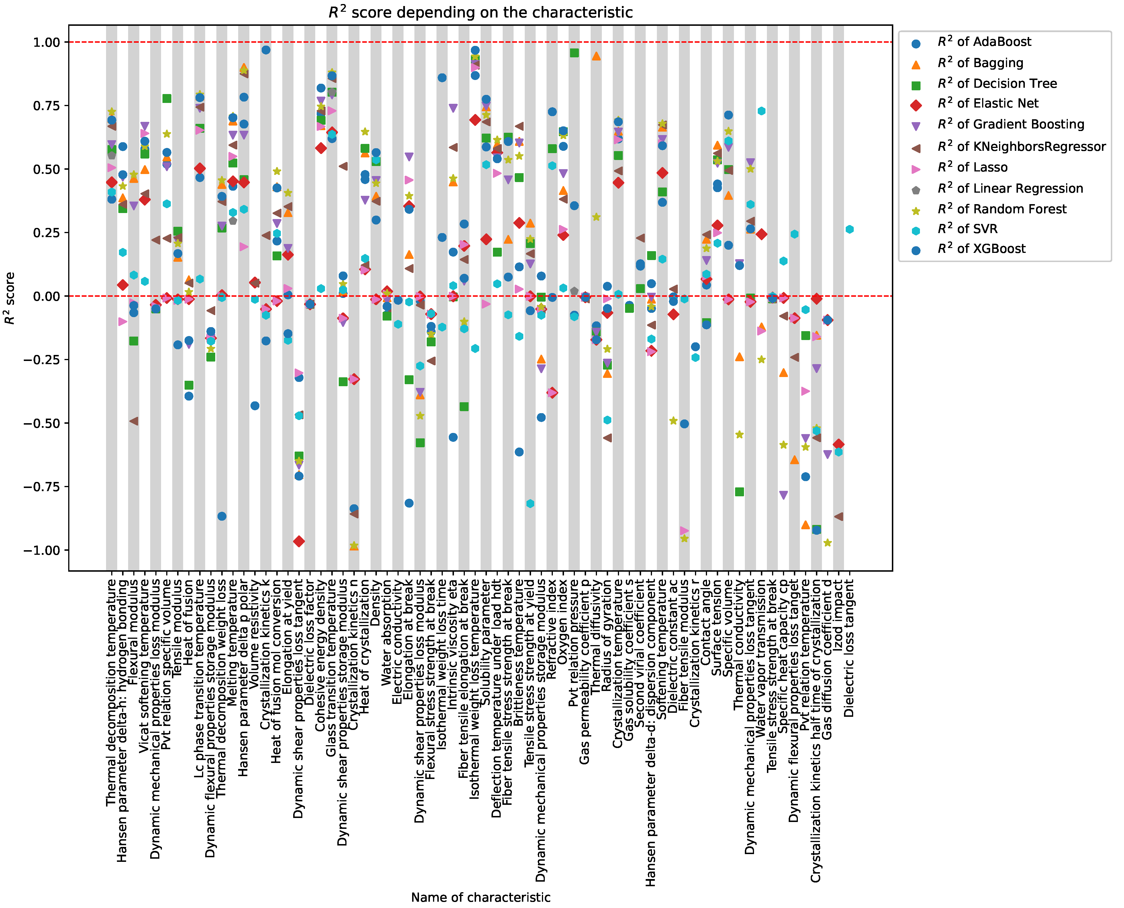
| Characteristic | Data Size 1 | Best Regressor | Max | MPE |
|---|---|---|---|---|
| Glass transition temperature | 8092 | Random Forest | 0.88 | 1.23 |
| Thermal decomposition temperature | 6325 | Random Forest | 0.73 | 2.25 |
| Melting temperature | 3844 | Random Forest | 0.71 | 1.05 |
| Intrinsic viscosity ETA | 1978 | Gradient Boosting | 0.74 | |
| Specific volume | 1739 | XGBoost | 0.71 | 2.75 |
| Density | 1739 | XGBoost | 0.56 | 0.5 |
| Elongation at break | 1139 | Gradient Boosting | 0.55 | |
| LC phase transition temperature | 961 | Random Forest | 0.79 | 3.02 |
| Softening temperature | 777 | Random Forest | 0.68 | 20.73 |
| Refractive index | 685 | XGBoost | 0.73 | 0.91 |
| Crystallization temperature | 457 | Random Forest | 0.69 | 6.3 |
| Surface tension | 348 | Bagging | 0.59 | 0.06 |
| Solubility parameter | 324 | XGBoost | 0.77 | 0.04 |
| Cohesive energy density | 324 | XGBoost | 0.82 | 0.96 |
| Dynamic mechanical properties loss tangent | 301 | Gradient Boosting | 0.52 | |
| Isothermal weight loss temperature | 273 | XGBoost | 0.97 | 0.13 |
| Isothermal weight loss time | 228 | XGBoost | 0.86 | |
| Oxygen index | 176 | XGBoost | 0.65 | 12.24 |
| Dynamic shear properties storage modulus | 141 | KNeighborsRegressor | 0.51 | |
| Heat of crystallization | 124 | Random Forest | 0.65 | |
| Deflection temperature under load HDT | 99 | Random Forest | 0.61 | 4.0 |
| Fiber tensile stress strength at break | 91 | Decision Tree | 0.63 | 1.1 |
| Vicat softening temperature | 82 | Gradient Boosting | 0.67 | 0.45 |
| Brittleness temperature | 81 | KNeighborsRegressor | 0.67 | 1.2 |
| Thermal diffusivity | 80 | Bagging | 0.94 | 4.13 |
| Water vapor transmission | 73 | SVR | 0.73 | |
| Hansen parameter delta p polar | 59 | Bagging | 0.9 | 0.45 |
| Hansen parameter delta-h: hydrogen bonding | 59 | AdaBoost | 0.59 | 2.56 |
| Crystallization kinetics k | 59 | XGBoost | 0.97 | |
| PVT relation specific volume | 56 | Decision Tree | 0.78 | 0.01 |
| PVT relation pressure | 53 | Decision Tree | 0.96 |
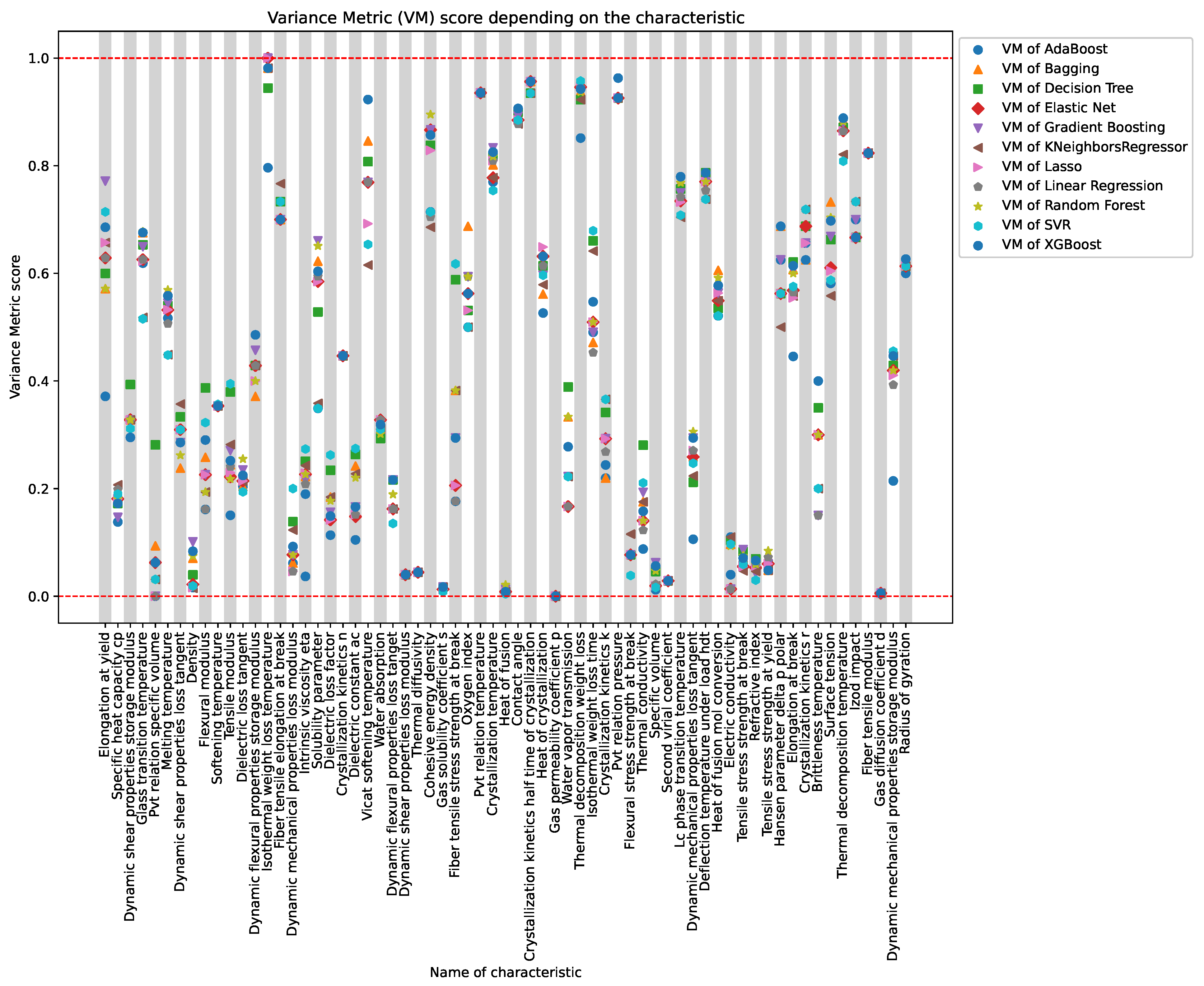
| Characteristic | Data Size 1 | Best Regressor | Max VM |
|---|---|---|---|
| Isothermal weight loss temperature | 219 | Elastic Net | 1.0 |
| PVT relation pressure | 26 | AdaBoost | 0.96 |
| Thermal decomposition weight loss | 3567 | SVR | 0.96 |
| Crystallization kinetics half time of crystallization | 26 | AdaBoost | 0.96 |
| PVT relation temperature | 26 | AdaBoost | 0.94 |
| Vicat softening temperature | 56 | Random Forest | 0.92 |
| Contact angle | 116 | Random Forest | 0.91 |
| Cohesive energy density | 219 | Random Forest | 0.9 |
| Thermal decomposition temperature | 2968 | XGBoost | 0.89 |
| Crystallization temperature | 331 | Gradient Boosting | 0.83 |
| Fiber tensile modulus | 40 | AdaBoost | 0.82 |
| Deflection temperature under load HDT | 38 | Bagging | 0.79 |
| LC phase transition temperature | 430 | XGBoost | 0.78 |
| Elongation at yield | 49 | Gradient Boosting | 0.77 |
| Fiber tensile elongation at break | 31 | KNeighborsRegressor | 0.77 |
| Izod impact | 23 | KNeighborsRegressor | 0.73 |
| Surface tension | 176 | Bagging | 0.73 |
| Crystallization kinetics r | 21 | KNeighborsRegressor | 0.72 |
| Oxygen index | 144 | Bagging | 0.69 |
| Hansen parameter delta p polar | 43 | Bagging | 0.69 |
| Isothermal weight loss time | 175 | SVR | 0.68 |
| Glass transition temperature | 6278 | Random Forest | 0.68 |
| Solubility parameter | 218 | Gradient Boosting | 0.66 |
| Heat of crystallization | 67 | Lasso | 0.65 |
| Radius of gyration | 45 | Bagging | 0.63 |
| Elongation at break | 854 | Decision Tree | 0.62 |
| Fiber tensile stress strength at break | 57 | SVR | 0.62 |
| Heat of fusion mol conversion | 154 | Bagging | 0.61 |
| Melting temperature | 2182 | Random Forest | 0.57 |
Disclaimer/Publisher’s Note: The statements, opinions and data contained in all publications are solely those of the individual author(s) and contributor(s) and not of MDPI and/or the editor(s). MDPI and/or the editor(s) disclaim responsibility for any injury to people or property resulting from any ideas, methods, instructions or products referred to in the content. |
© 2023 by the authors. Licensee MDPI, Basel, Switzerland. This article is an open access article distributed under the terms and conditions of the Creative Commons Attribution (CC BY) license (https://creativecommons.org/licenses/by/4.0/).
Share and Cite
Malashin, I.P.; Tynchenko, V.S.; Nelyub, V.A.; Borodulin, A.S.; Gantimurov, A.P. Estimation and Prediction of the Polymers’ Physical Characteristics Using the Machine Learning Models. Polymers 2024, 16, 115. https://doi.org/10.3390/polym16010115
Malashin IP, Tynchenko VS, Nelyub VA, Borodulin AS, Gantimurov AP. Estimation and Prediction of the Polymers’ Physical Characteristics Using the Machine Learning Models. Polymers. 2024; 16(1):115. https://doi.org/10.3390/polym16010115
Chicago/Turabian StyleMalashin, Ivan Pavlovich, Vadim Sergeevich Tynchenko, Vladimir Aleksandrovich Nelyub, Aleksei Sergeevich Borodulin, and Andrei Pavlovich Gantimurov. 2024. "Estimation and Prediction of the Polymers’ Physical Characteristics Using the Machine Learning Models" Polymers 16, no. 1: 115. https://doi.org/10.3390/polym16010115
APA StyleMalashin, I. P., Tynchenko, V. S., Nelyub, V. A., Borodulin, A. S., & Gantimurov, A. P. (2024). Estimation and Prediction of the Polymers’ Physical Characteristics Using the Machine Learning Models. Polymers, 16(1), 115. https://doi.org/10.3390/polym16010115