
Single and Multiple Gate Design Optimization Algorithm for Improving the Effectiveness of Fiber Reinforcement in the Thermoplastic Injection Molding Process

 ,
, 

Abstract
1. Introduction
2. Materials and Methods
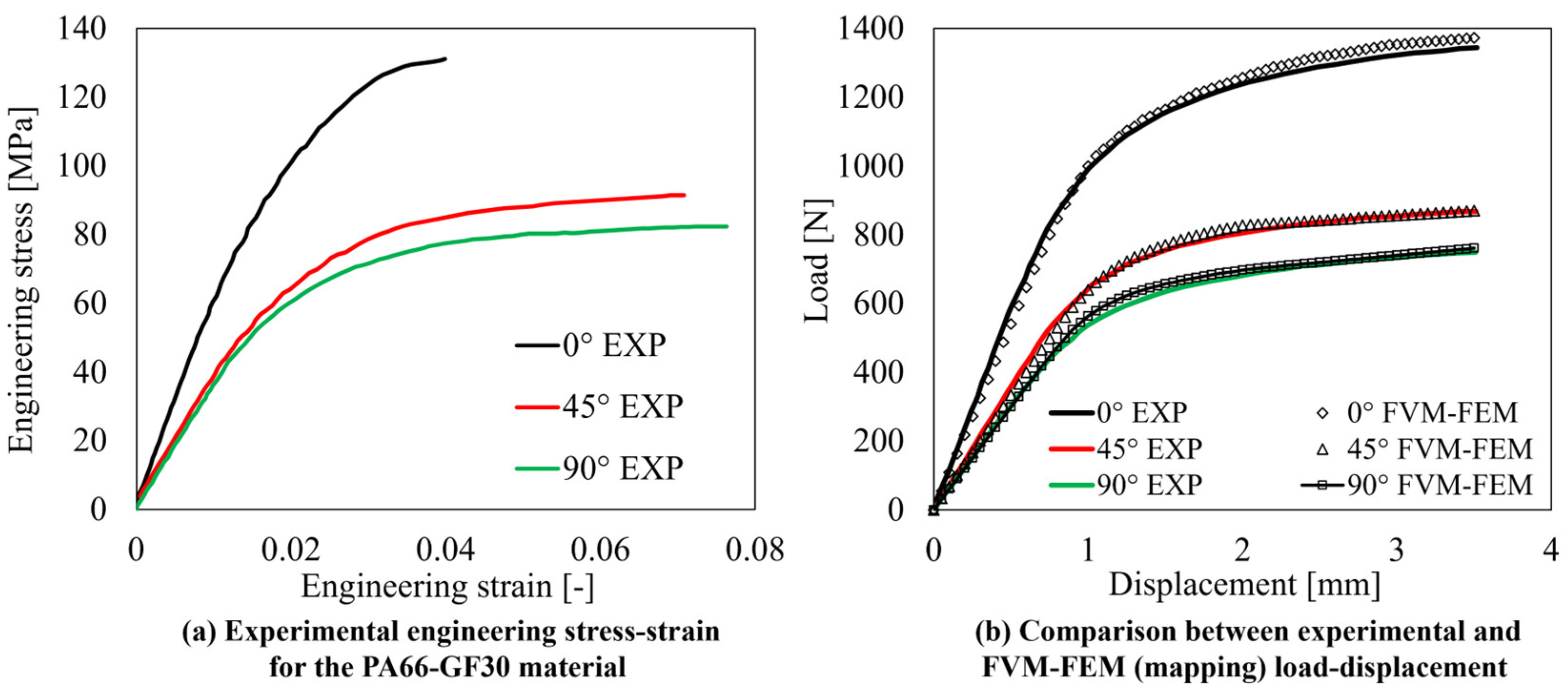
2.1. PA66-30GF Properties and FVM Simulation Settings
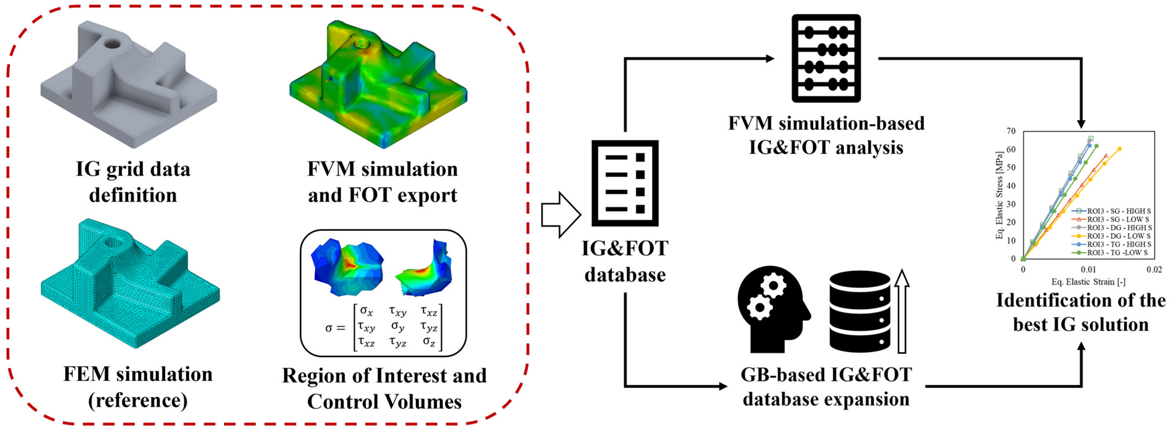
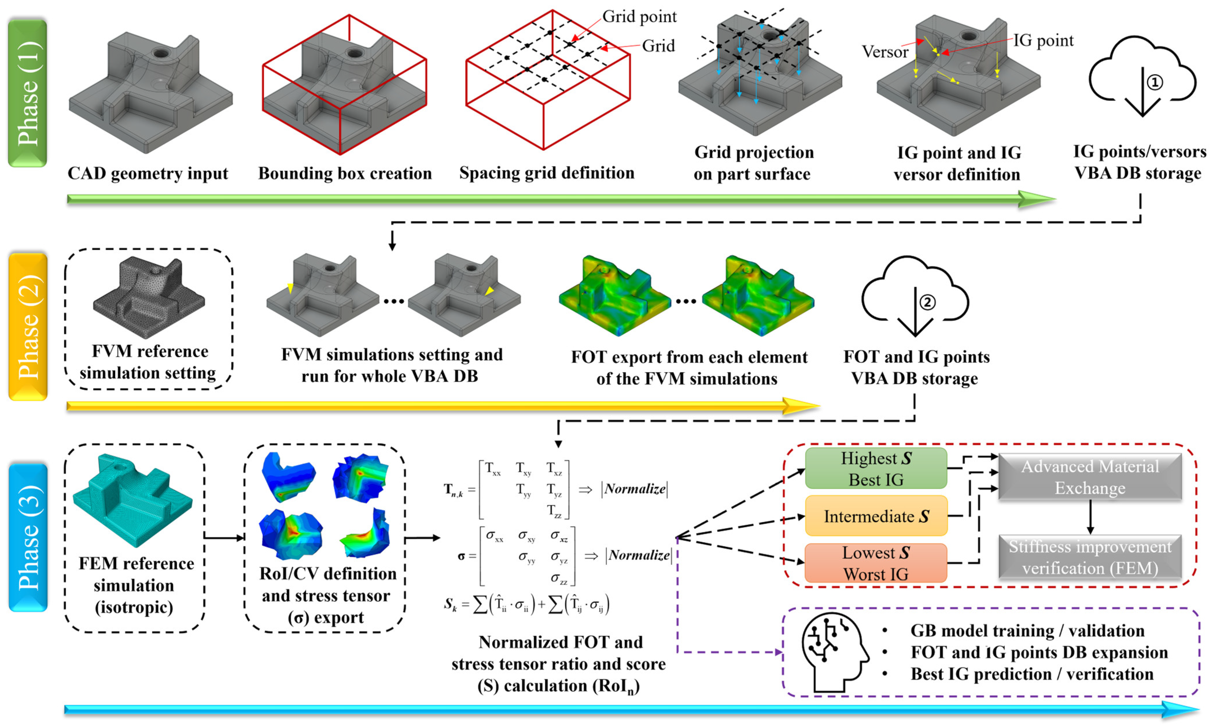
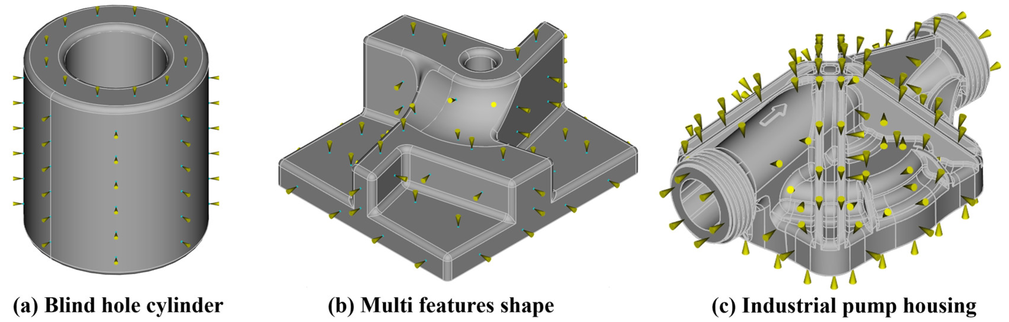
2.2. Single and Multiple Injection Gate Design Algorithm
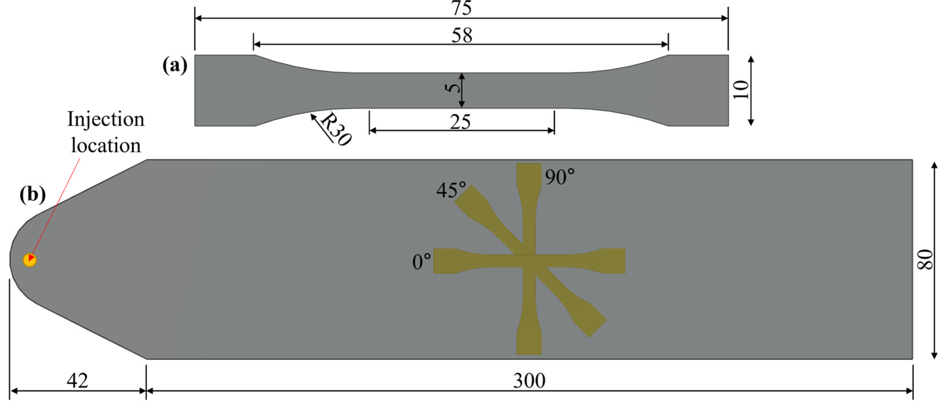
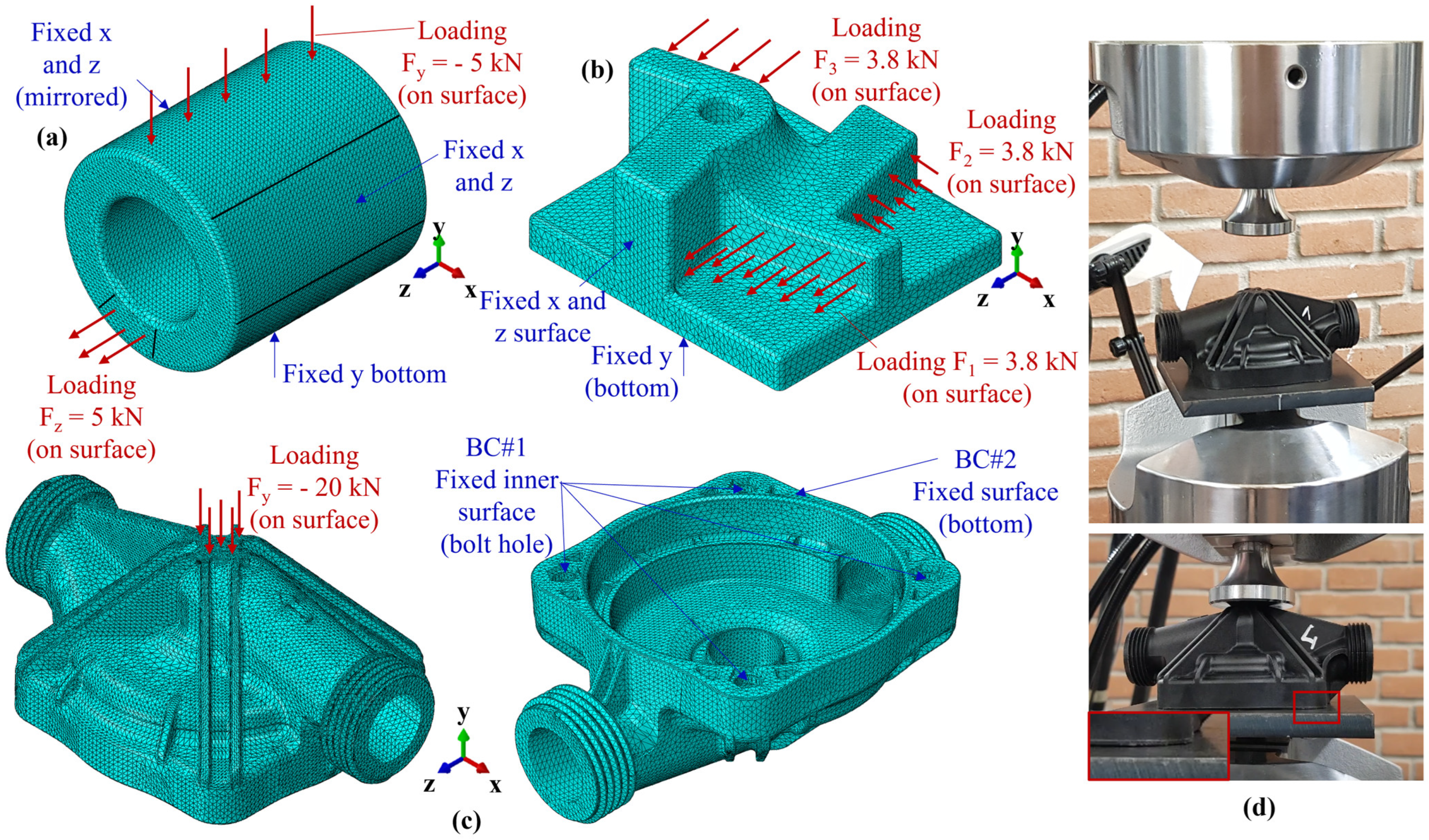
2.3. FEM Simulation Settings and Validation Experiments
3. Results
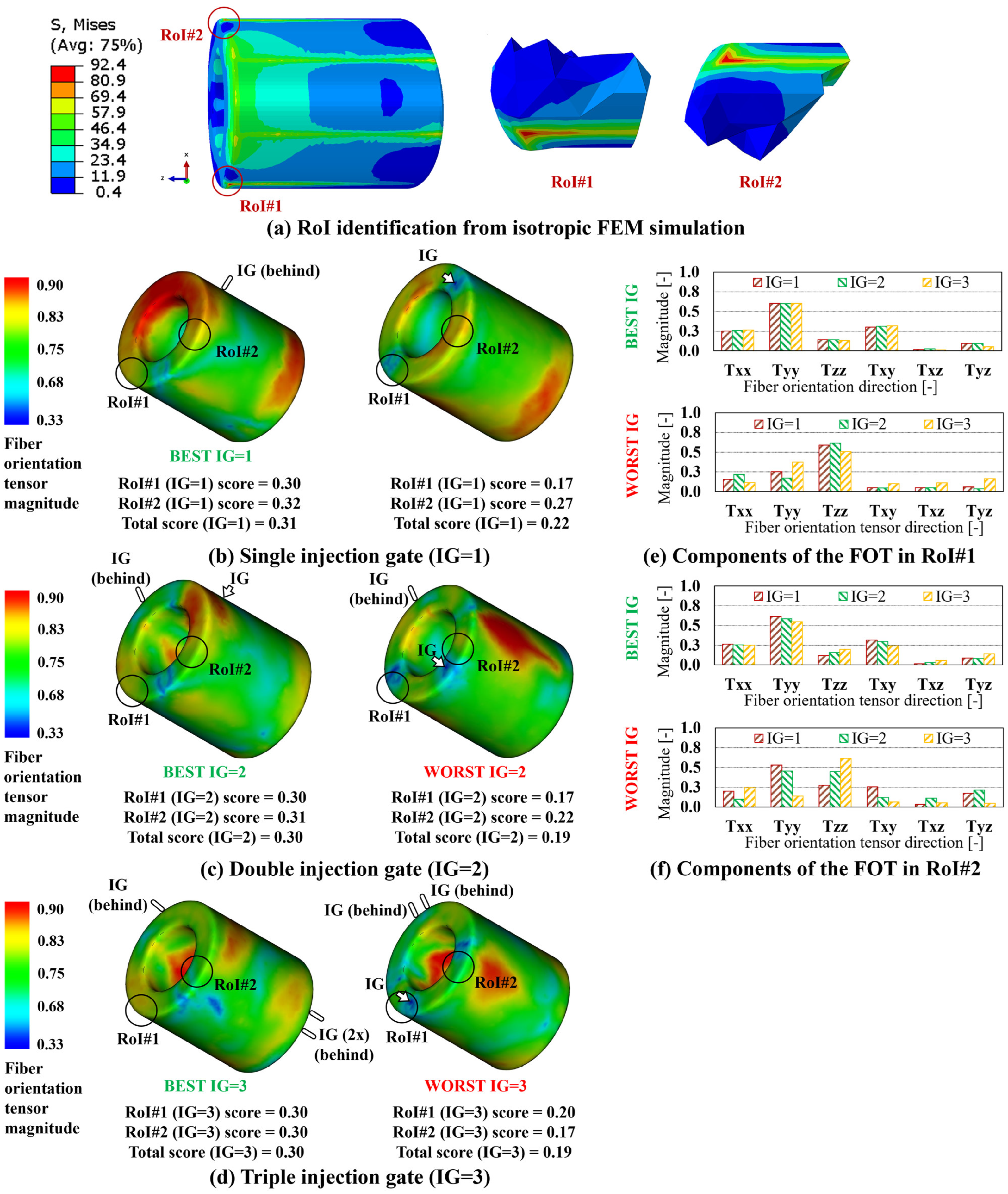
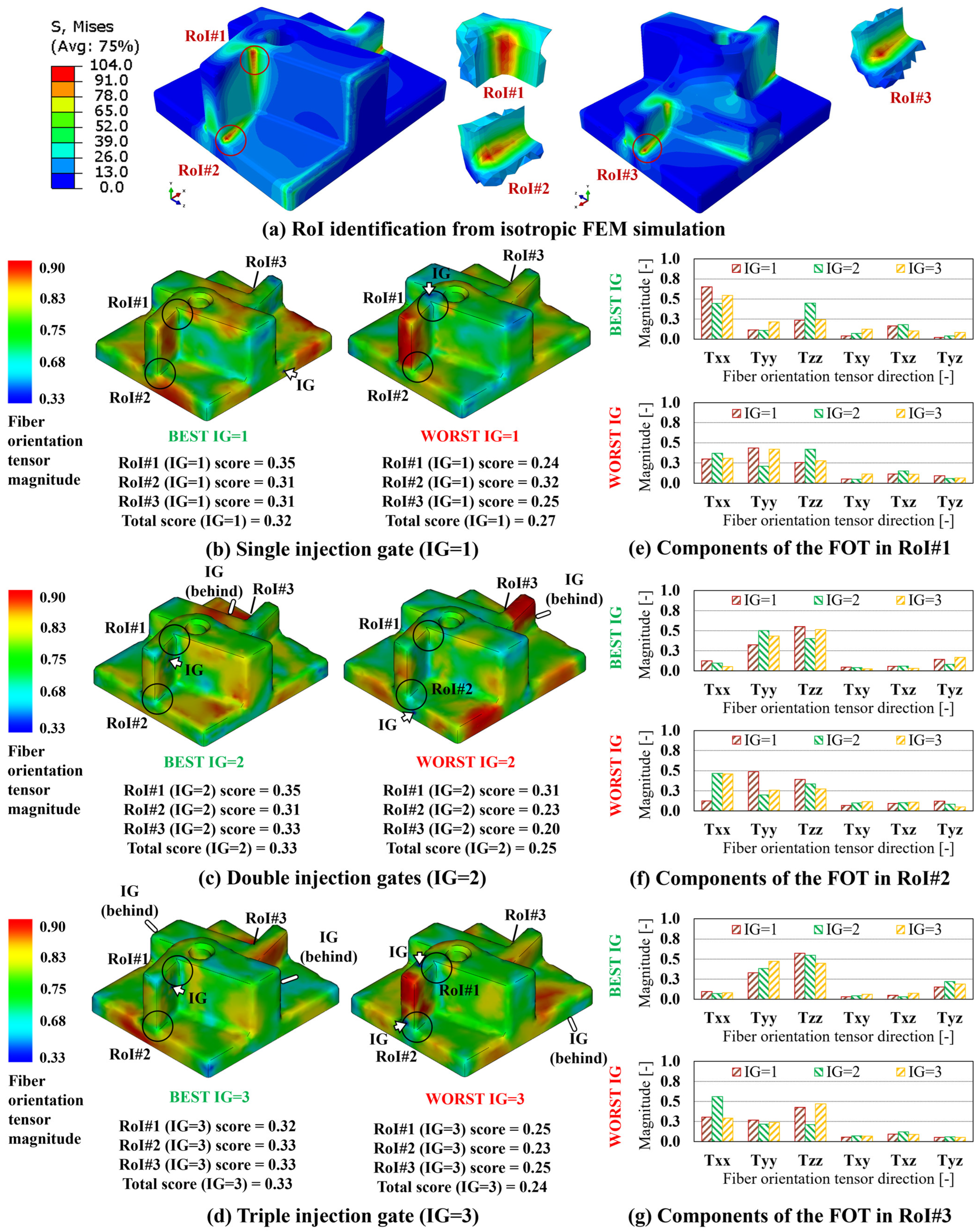
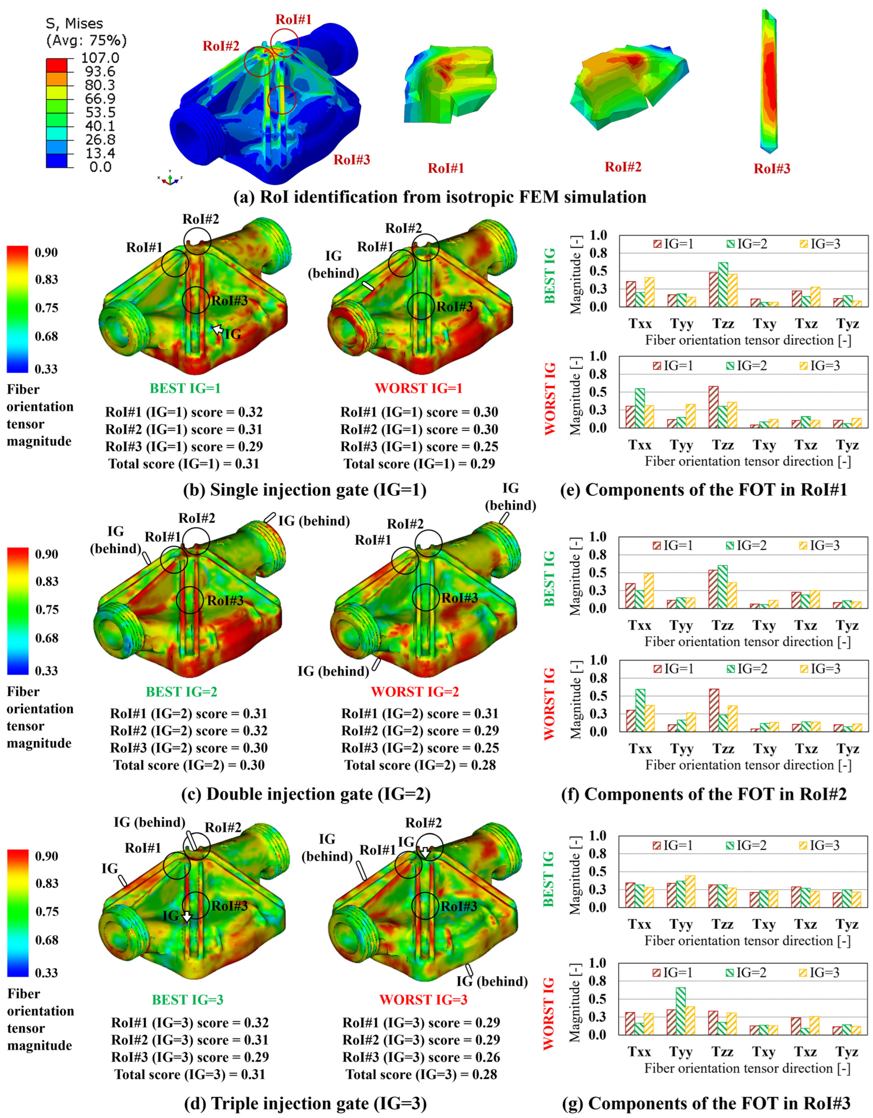
3.1. IG Solutions and RoI Scores Calculation
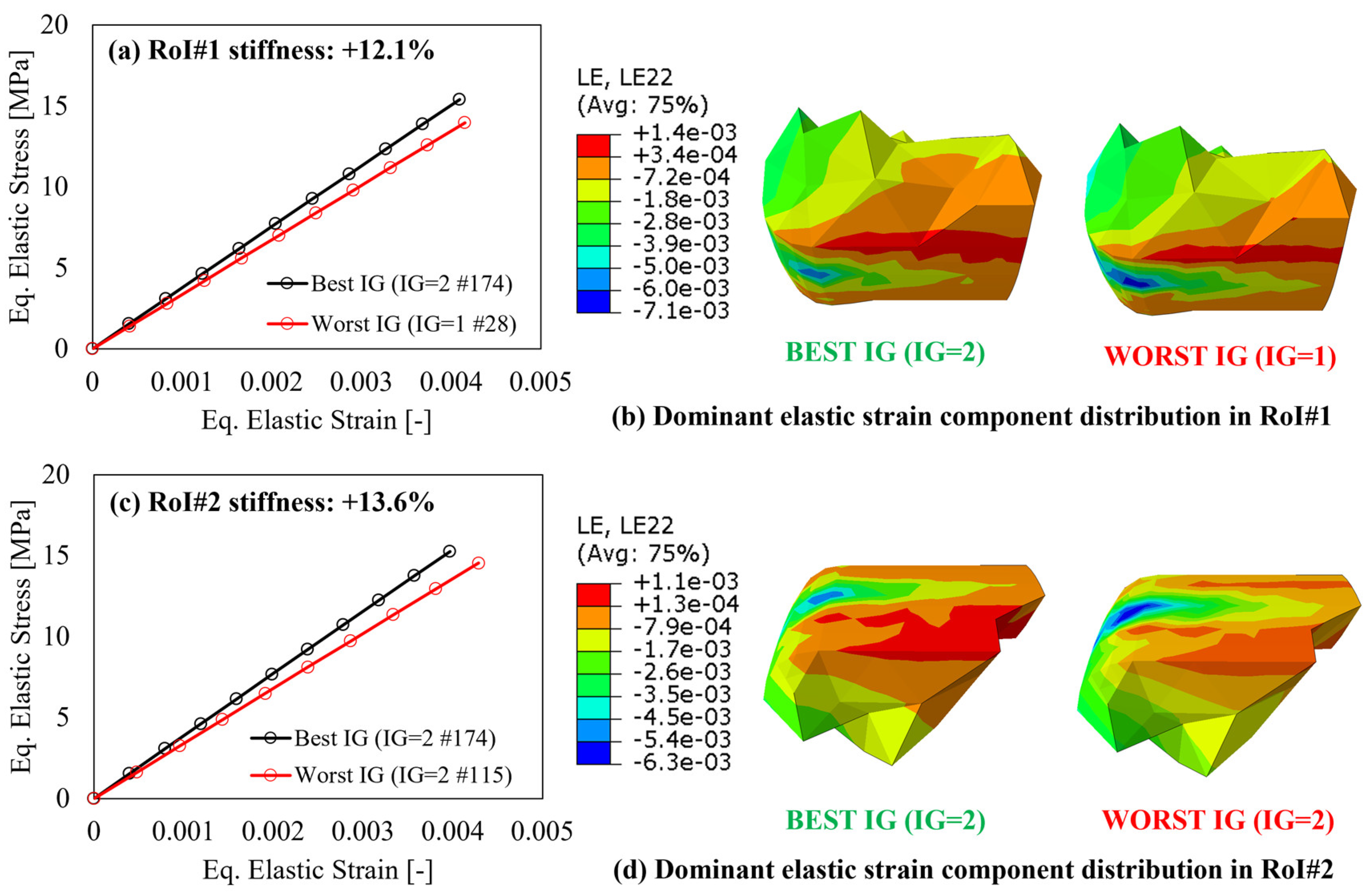
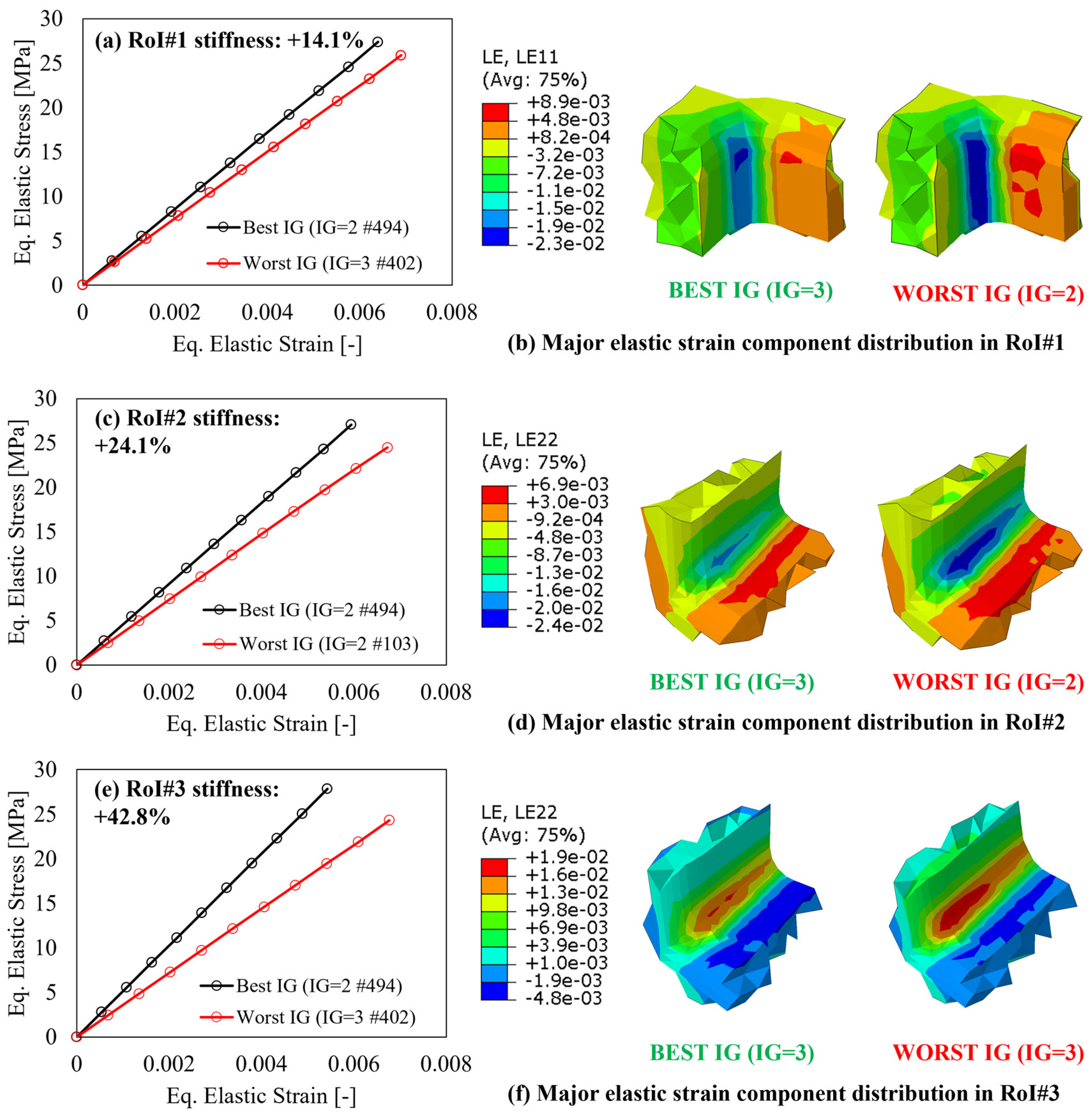
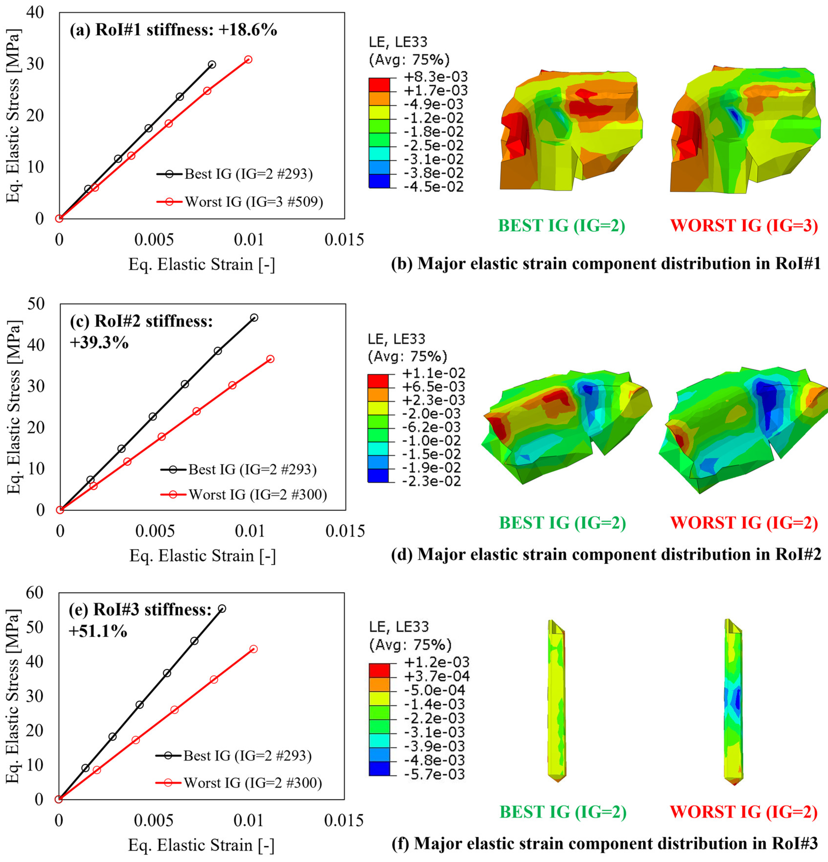
3.2. FVM-FEM-Based IG Design and Stiffness Improvement
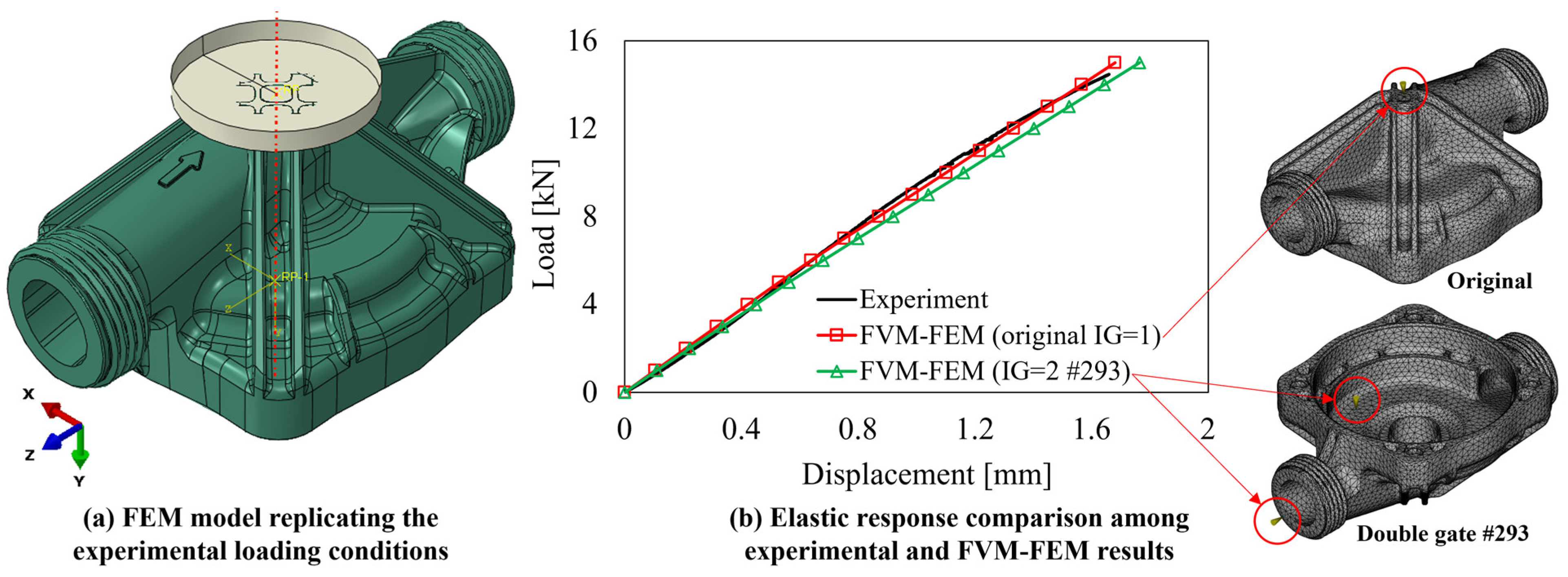
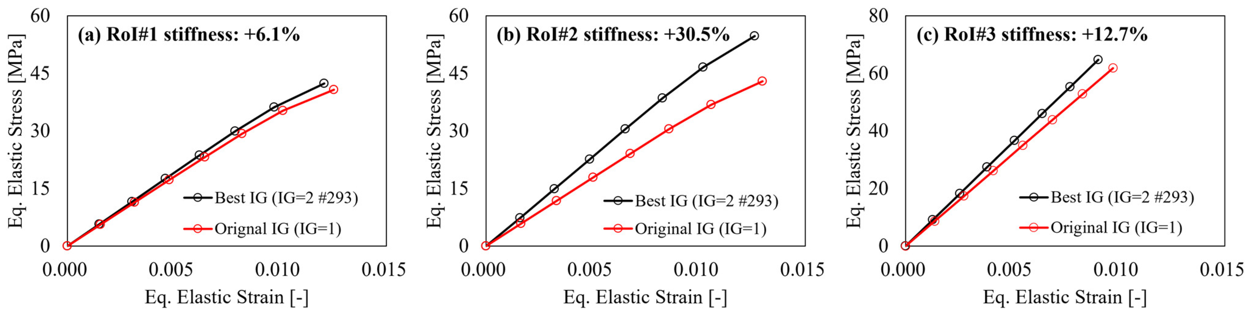
3.3. FVM/FEM Validation and Benefits of IG Design Improvement
3.4. Gradient Boosting-Based IG Design Optimization
4. Discussion
5. Conclusions
Author Contributions
Funding
Institutional Review Board Statement
Data Availability Statement
Conflicts of Interest
References
- Evens, T.; Bex, G.J.; Yigit, M.; De Keyzer, J.; Desplentere, F.; Van Bael, A. The influence of mechanical recycling on properties in injection molding of fiber-reinforced polypropylene. Int. Polym. Process. 2019, 34, 398–407. [Google Scholar] [CrossRef]
- Gajdoš, I.; Slota, J.; Kaščák, L.; Grytsenko, O.; Jachowicz, T. Utilization of analytical methods for the failure analysis of injection molded parts. Acta Metall. Slov. 2020, 26, 122–125. [Google Scholar] [CrossRef]
- Fu, Y.; Yao, X. A review on manufacturing defects and their detection of fiber reinforced resin matrix composites. Compos. Part C Open Access 2022, 8, 100276. [Google Scholar] [CrossRef]
- Zhao, N.; Lian, J.; Wang, P.; Xu, Z. Recent progress in minimizing the warpage and shrinkage deformations by the optimization of process parameters in plastic injection molding: A review. Int. J. Adv. Manuf. Technol. 2022, 120, 85–101. [Google Scholar] [CrossRef] [PubMed]
- Hashimoto, S.; Kitayama, S.; Takano, M.; Kubo, Y.; Aiba, S. Simultaneous optimization of variable injection velocity profile and process parameters in plastic injection molding for minimizing weldline and cycle time. J. Adv. Mech. Des. Syst. Manuf. 2020, 14, JAMDSM0029. [Google Scholar] [CrossRef]
- Jeong, E.; Kim, Y.; Hong, S.; Yoon, K.; Lee, S. Innovative Injection Molding Process for the Fabrication of Woven Fabric Reinforced Thermoplastic Composites. Polymers 2022, 14, 1577. [Google Scholar] [CrossRef]
- Pegoretti, A. Recycling concepts for short-fiber-reinforced and particle-filled thermoplastic composites: A review. Adv. Ind. Eng. Polym. Res. 2021, 4, 93–104. [Google Scholar] [CrossRef]
- Fonseca, J.H.; Lee, J.; Jang, W.; Han, D.; Kim, N.; Lee, H. Manufacturability-constrained optimization for enhancing quality and suitability of injection-molded short fiber-reinforced plastic/metal hybrid automotive structures. Struct. Multidiscip. Optim. 2023, 66, 113. [Google Scholar] [CrossRef]
- Mao, H.; Wang, Y.; Yang, D. Study of injection molding process simulation and mold design of automotive back door panel. J. Mech. Sci. Technol. 2022, 36, 2331–2344. [Google Scholar] [CrossRef]
- Ishikawa, T.; Amaoka, K.; Masubuchi, Y.; Yamamoto, T.; Yamanaka, A.; Arai, M.; Takahashi, J. Overview of automotive structural composites technology developments in Japan. Compos. Sci. Technol. 2018, 155, 221–246. [Google Scholar] [CrossRef]
- Quagliato, L.; Kim, Y.; Fonseca, J.H.; Han, D.; Yun, S.; Lee, H.; Park, N.; Lee, H.; Kim, N. The influence of fiber orientation and geometry-induced strain concentration on the fatigue life of short carbon fibers reinforced polyamide-6. Mater. Des. 2020, 190, 108569. [Google Scholar] [CrossRef]
- Lee, C.S.; Kim, H.J.; Amanov, A.; Choo, J.H.; Kim, Y.K.; Cho, I.S. Investigation on very high cycle fatigue of PA66-GF30 GFRP based on fiber orientation. Compos. Sci. Technol. 2019, 180, 94–100. [Google Scholar] [CrossRef]
- Vicente, M.A.; Ruiz, G.; González, D.C.; Mínguez, J.; Tarifa, M.; Zhang, X. Effects of fiber orientation and content on the static and fatigue behavior of SFRC by using CT-Scan technology. Int. J. Fatigue 2019, 128, 105178. [Google Scholar] [CrossRef]
- Quagliato, L.; Lee, J.; Fonseca, J.H.; Han, D.; Lee, H.; Kim, N. Influences of stress triaxiality and local fiber orientation on the failure strain for injection-molded carbon fiber reinforced polyamide-6. Eng. Fract. Mech. 2021, 250, 107784. [Google Scholar] [CrossRef]
- Tanaka, K.; Kitano, T.; Egami, N. Effect of fiber orientation on fatigue crack propagation in short-fiber reinforced plastics. Eng. Fract. Mech. 2014, 123, 44–58. [Google Scholar] [CrossRef]
- Lee, J.; Lee, H.; Kim, N. Fiber Orientation and Strain Rate-Dependent Tensile and Compressive Behavior of Injection Molded Polyamide-6 Reinforced with 20% Short Carbon Fiber. Polymers 2023, 15, 738. [Google Scholar] [CrossRef]
- Quagliato, L.; Ricotta, M.; Zappalorto, M.; Ryu, S.C.; Kim, N. Notch effect in 20% short carbon fibre-PA reinforced composites under quasi-static tensile loads. Theor. Appl. Fract. Mech. 2022, 122, 103649. [Google Scholar] [CrossRef]
- Ricotta, M.; Sorgato, M.; Zappalorto, M. Tensile and compressive quasi-static behaviour of 40% short glass fibre—PPS reinforced composites with and without geometrical variations. Theor. Appl. Fract. Mech. 2021, 114, 102990. [Google Scholar] [CrossRef]
- Huang, D.; Zhao, X. A generalized distribution function of fiber orientation for injection molded composites. Compos. Sci. Technol. 2020, 188, 107999. [Google Scholar] [CrossRef]
- Wang, J.; O’Gara, J.F.; Tucker, C.L. An objective model for slow orientation kinetics in concentrated fiber suspensions: Theory and rheological evidence. J. Rheol. 2008, 52, 1179–1200. [Google Scholar] [CrossRef]
- Phelps, J.H.; Tucker, C.L. An anisotropic rotary diffusion model for fiber orientation in short- and long-fiber thermoplastics. J. Nonnewton. Fluid Mech. 2009, 156, 165–176. [Google Scholar] [CrossRef]
- Favaloro, A.J.; Tucker, C.L. Analysis of anisotropic rotary diffusion models for fiber orientation. Compos. Part A Appl. Sci. Manuf. 2019, 126, 105605. [Google Scholar] [CrossRef]
- Ivan, R.; Sorgato, M.; Zanini, F.; Lucchetta, G. Improving Numerical Modeling Accuracy for Fiber Orientation and Mechanical Properties of Injection Molded Glass Fiber Reinforced Thermoplastics. Materials 2022, 15, 4720. [Google Scholar] [CrossRef] [PubMed]
- Tseng, H.C.; Chang, R.Y.; Hsu, C.H. Comparison of recent fiber orientation models in injection molding simulation of fiber-reinforced composites. J. Thermoplast. Compos. Mater. 2020, 33, 35–52. [Google Scholar] [CrossRef]
- Hopmann, C.; Weber, M.; Van Haag, J.; Schöngart, M. A validation of the fibre orientation and fibre length attrition prediction for long fibre-reinforced thermoplastics. AIP Conf. Proc. 2015, 1664, 050008. [Google Scholar] [CrossRef]
- Wang, J.; Jin, X. Comparison of recent Fiber Orientation Models in Autodesk Moldflow Insight Simulations with measured Fiber Orientation Data. In Proceedings of the Polymer Processing Society 26th Annual Meeting, Banff, AB, Canada, 4–8 July 2010. [Google Scholar]
- Zhai, M.; Lam, Y.; Au, C. Gate location optimization scheme for plastic injection molding. E-Polymers 2009, 9, 127. [Google Scholar] [CrossRef]
- Zhai, M.; Xie, Y. A study of gate location optimization of plastic injection molding using sequential linear programming. Int. J. Adv. Manuf. Technol. 2010, 49, 97–103. [Google Scholar] [CrossRef]
- Wang, J.; Mao, Q. Methodology Based on the PVT Behavior of Polymer for Injection Molding. Adv. Polym. Technol. 2012, 32, 474–485. [Google Scholar] [CrossRef]
- Huszar, M.; Belblidia, F.; Davies, H.M.; Arnold, C.; Bould, D.; Sienz, J. Sustainable injection moulding: The impact of materials selection and gate location on part warpage and injection pressure. Sustain. Mater. Technol. 2015, 5, 1–8. [Google Scholar] [CrossRef]
- Li, K.; Yan, S.L.; Pan, W.F.; Zhao, G. Optimization of fiber-orientation distribution in fiber-reinforced composite injection molding by Taguchi, back propagation neural network, and genetic algorithm-particle swarm optimization. Adv. Mech. Eng. 2017, 9, 1687814017719221. [Google Scholar] [CrossRef]
- Mirandola, I.; Berti, G.A.; Caracciolo, R.; Lee, S.; Kim, N.; Quagliato, L. Machine learning-based models for the estimation of the energy consumption in metal forming processes. Metals 2021, 11, 833. [Google Scholar] [CrossRef]
- Lee, S.; Park, J.; Kim, N.; Lee, T.; Quagliato, L. Extreme gradient boosting-inspired process optimization algorithm for manufacturing engineering applications. Mater. Des. 2023, 226, 111625. [Google Scholar] [CrossRef]
- Moayyedian, M.; Dinc, A.; Mamedov, A. Optimization of injection-molding process for thin-walled polypropylene part using artificial neural network and Taguchi techniques. Polymers 2021, 13, 4158. [Google Scholar] [CrossRef]
- Finkeldey, F.; Volke, J.; Zarges, J.C.; Heim, H.P.; Wiederkehr, P. Learning quality characteristics for plastic injection molding processes using a combination of simulated and measured data. J. Manuf. Process. 2020, 60, 134–143. [Google Scholar] [CrossRef]
- Isaincu, A.; Dan, M.; Ungureanu, V.; Marsavina, L. Numerical investigation on the influence of fiber orientation mapping procedure to the mechanical response of short-fiber reinforced composites using Moldflow, Digimat and Ansys software. Mater. Today Proc. 2020, 45, 4304–4309. [Google Scholar] [CrossRef]
- Folgar, F.; Tucker, C.L. Orientation Behavior of Fibers in Concentrated Suspensions. J. Reinf. Plast. Compos. 1984, 3, 98–119. [Google Scholar] [CrossRef]


| Symbol [Unit] | Definition | Value |
|---|---|---|
| Strength coefficient | 60.81 | |
| Hardening exponent | 15.97 | |
| Polymer matrix elastic modulus | 2.21 | |
| Fibers’ elastic modulus | 36.52 | |
| Weight factor for the fiber direction | 1.42 | |
| Weight factor for the direction normal to the fibers | 1.17 | |
| First eigenvalue of the fiber orientation matrix in the region of the model with the highest fiber alignment with the polymer flow | 0.85 |
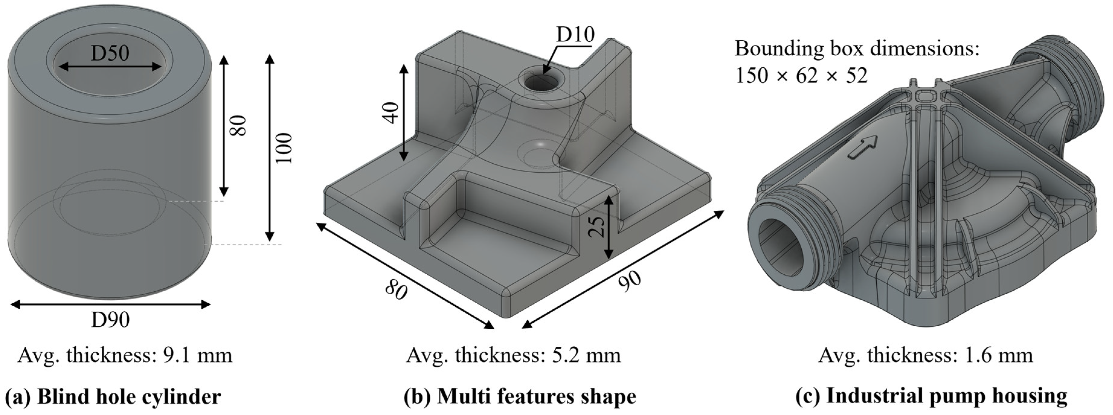
| Parameter | Injection Molded Plate | Blind Hole Cylinder | Multi Features Shape | Industrial Pump Housing |
|---|---|---|---|---|
| Molten material temperature | 290 °C | 285 °C | 285 °C | |
| Mold temperature | 85 °C | 110 °C | 110 °C | |
| Injection time | 1.51 s | Automatic | Automatic | |
| Velocity/pressure switch-over | 98.7% | 99% | 98% | |
| Packing–cooling time | 10 s | 20 s | 30 s | |
| Post-pressure | 80% | 80% | 85% | |
| Component | IG = 1 | IG = 2 | IG = 3 |
|---|---|---|---|
| Blind hole cylinder | 90 | 90 | 90 |
| Multi features shape | 110 | 110 | 110 |
| Industrial pump housing | 160 | 160 | 160 |
| Parameter | Blind Hole Cylinder | Multi Features Shape | Industrial Pump Housing |
|---|---|---|---|
| Max depth | 10 | 9 | 9 |
| Min samples leaf | 7 | 7 | 7 |
| Min samples split | 8 | 6 | 5 |
| Estimators number (M) | 100 | 100 | 100 |
| Learning rate (η) | 0.1 | 0.1 | 0.1 |
| Loss function (δ) | 0.9 | 0.9 | 0.9 |
| Training accuracy (5-fold average) | 94% | 97.7% | 98.1% |
| Validation accuracy (5-fold average) | 91.4% | 97.4% | 97.8% |
| IG Coordinates | Blind Hole Cylinder | Multi Features Shape | Industrial Pump Housing | |||||||
|---|---|---|---|---|---|---|---|---|---|---|
| x | y | z | x | y | z | x | y | z | ||
| Pre GB-ML | IG = 2 (#1) | 76.8 | 76.8 | 72.0 | 13.7 | 28.0 | 41.6 | 10.45 | 13.96 | 36.8 |
| IG = 2 (#2) | 13.8 | 76.8 | 87 | 60 | 10 | 60 | 22.7 | 25.2 | 57.2 | |
| Post GB-ML | IG = 2 (#1) | 73.9 | 79.5 | 67.4 | 63.8 | 10 | 56 | 15.5 | 18.4 | 45.8 |
| IG = 2 (#2) | 60.6 | 79.7 | 0 | 12.9 | 31.6 | 41.8 | 24.8 | 25.2 | 36.0 | |
| Average ROI Stiffness improvement | 8.6% | 5.1% | 6.3% | |||||||
Disclaimer/Publisher’s Note: The statements, opinions and data contained in all publications are solely those of the individual author(s) and contributor(s) and not of MDPI and/or the editor(s). MDPI and/or the editor(s) disclaim responsibility for any injury to people or property resulting from any ideas, methods, instructions or products referred to in the content. |
© 2023 by the authors. Licensee MDPI, Basel, Switzerland. This article is an open access article distributed under the terms and conditions of the Creative Commons Attribution (CC BY) license (https://creativecommons.org/licenses/by/4.0/).
Share and Cite
Perin, M.; Lim, Y.; Berti, G.A.; Lee, T.; Jin, K.; Quagliato, L. Single and Multiple Gate Design Optimization Algorithm for Improving the Effectiveness of Fiber Reinforcement in the Thermoplastic Injection Molding Process. Polymers 2023, 15, 3094. https://doi.org/10.3390/polym15143094
Perin M, Lim Y, Berti GA, Lee T, Jin K, Quagliato L. Single and Multiple Gate Design Optimization Algorithm for Improving the Effectiveness of Fiber Reinforcement in the Thermoplastic Injection Molding Process. Polymers. 2023; 15(14):3094. https://doi.org/10.3390/polym15143094
Chicago/Turabian StylePerin, Mattia, Youngbin Lim, Guido A. Berti, Taeyong Lee, Kai Jin, and Luca Quagliato. 2023. "Single and Multiple Gate Design Optimization Algorithm for Improving the Effectiveness of Fiber Reinforcement in the Thermoplastic Injection Molding Process" Polymers 15, no. 14: 3094. https://doi.org/10.3390/polym15143094
APA StylePerin, M., Lim, Y., Berti, G. A., Lee, T., Jin, K., & Quagliato, L. (2023). Single and Multiple Gate Design Optimization Algorithm for Improving the Effectiveness of Fiber Reinforcement in the Thermoplastic Injection Molding Process. Polymers, 15(14), 3094. https://doi.org/10.3390/polym15143094