Abstract
Periodic arrays in one, two, and three dimensions, made of magnetic spheres embedded in a fluid matrix, are considered in this study and utilized as phononic structures. The propagation of acoustic waves through these structures is analyzed experimentally, in low- and high-frequency region, via laser vibrometry, as well as standard underwater acoustic measurements. A first comparison to theoretical calculations obtained through multiple-scattering techniques and multipole models reveals a distinct behavior depending on the immersion fluid and/or frequency regime. Our results show that the elastodynamic response of these systems can be, under conditions, simply described by classical elastic theory without taking directly (ab initio) into account the magnetic character of the spherical particles. The structures considered above could offer several possibilities including facility of construction and use in filtering applications, but they are also of interest from a theoretical point of view, as a means to investigate the validity of several approximate theoretical descriptions.
Keywords:
phononic crystals; layer-multiple-scattering; magnetic spheres; Hertz contact; underwater acoustics; laser Doppler vibrometry PACS:
43.40.Fz; 46.40.Cd; 63.20.D-
1. Introduction
Phononic crystals are composite materials with a periodic modulation of their elastic properties (mass density and propagation velocities of the longitudinal and transverse elastic waves) leading to formation of frequency regions where the elastic waves cannot propagate whatever the direction of propagation, known as phononic band gaps. Though this property motivated the primary interest for these structures by analogy with energy band gaps in crystalline solids, in the last two decades, phononic crystals and related structures have become popular and continuously attract a growing interest [1,2], especially after the triggering of several new physical ideas such as cloaking [3], negative refraction [4], and acoustic and thermal diodes [5], often transferred from their electromagnetic counterpart, the photonic crystals.
Most of the work, experimental as well as theoretical, has initially been focused on structures with cylindrical scatterers embedded in a, solid or fluid, host medium, due to their facility of construction and relative simplicity in the theoretical description. However, systems with spherical or other finite-shape scatterers (ellipsoids, cubes, pillars, etc) become nowadays interesting since they offer the possibility of constructing low-dimensional arrays or metasurfaces [6], which are of practical importance for applications in small-sized devices. On the other hand, these kinds of scatterers are massively used at the nanoscale to fabricate three-dimensional (3D) colloidal crystals by self-assembly techniques [7,8,9], while experiments at macroscale are less frequent especially due to difficulties in fabrication. They concern mostly structures made of solid spheres immersed in a fluid (water or air) [4,10], apart from cases of all-solid [11] or all-fluid [12] component structures. In the above cases, spheres are not consolidated between each other to form a continuous closed periodic network. The latter constitutes a special category of the well-known granular media, merging the physics of periodic materials to that of the elastic contact between solids [13]. Periodic granular materials have been extensively studied up to now [14,15,16,17,18,19], especially from the point of view of the nonlinear waves appearing in the structures as a result of strong applied forces in static and dynamic regime. In these works, discrete models [15,16,17,18,19] or finite element techniques [14] are used for the theoretical description of the elastic response of the system.
Here, we propose the use of rare-earth permanent magnetic spheres to construct one, two, and three-dimensional phononic crystals. We exploit the magnetic force between adjacent spheres to keep the structure in touch, the network of spheres forming a solid continuous frame. These kinds of scatterers have already been used to construct one-dimensional chains made of an alternation of magnetic and not magnetic supercells (each of them consisting of several spheres) [20]. In our case, the applied magnetic forces are weak, thus allowing for operation in the linear elastic regime. We study, experimentally and theoretically, the elastic response of the arrays and analyze the underlying physical mechanisms. The elastic contact between spheres is not involved in our theoretical calculations based on multiple-scattering techniques that utilize the vectorial multipole character of the elastic wavefields, not taken into account in the discrete models. Our results show that the elastic contact effect is not prominent in some cases, depending on the manner the system is excited and/or the immersion fluid.
2. Method of Calculation
We shall briefly outline the basic ideas of the method used for the theoretical calculations, namely the layer-multiple-scattering method (LMS) as applied to phononic crystals and related structures [21,22]. This method follows the principles of the KKR formalism [23,24], first applied to describe the electronic structure of crystalline solids and appropriately modified to treat also surface state physical phenomena [25]. Its power and efficiency lie in the multipole character of the expansions of the waves, modes and all derived physical quantities, thus offering the possibility of revealing the underlying physical mechanisms.
The essence of the method is tightly connected to the multiple scattering of the elastic waves propagating in a host medium containing more than one, well-defined and non-overlapping inclusions (scatterers) in its interior, the scatterers having different elastic parameters from those of the matrix. Two key quantities are necessary in this rigorous, exact description: the transition, -matrix, describing the scattering of an elastic wave by a single specific object, and the free propagator matrix, Ω, describing the propagation of an elastic wave from one point of the host medium to an other. For a more qualitative description of the method, the reader can refer to, e.g., References [26,27], while the full quantitative, detailed and complete description can be found in [21,22].
Before describing the essential steps of the LMS method, we note that this method can treat infinite periodic structures, or even heterostructures, consisting of a sequence of layers, along a specific direction, say z-axis. Each layer—a two-dimensional (2D) array of spheres embedded in a host matrix, an interface separating two homogeneous and isotropic media, a homogeneous and isotropic plate, or a combination of them—is supposed to extend to infinity along -plane and must have the same 2D periodicity (if any), thus leading to conservation of the wavevector component, , parallel to the layer’s characteristic surface (-plane). The LMS, being an on-shell method, calculates all necessary physical quantities for a given, specific frequency ω (we assume an dependence), each calculation being independent. Thus, ω and constitute two external variables to be determined for each calculation and all calculated quantities depend on these two parameters.
A second characteristic of major importance for the LMS method is the combination of two vector representations, the vector spherical-wave basis characterized by the angular momentum numbers ℓ and m, and the vector plane-wave basis characterized by the 2D reciprocal lattice vectors defining the diffracted beams. For instance, for a square (2D) array with lattice constant a, , where .
The following basic steps are involved in the LMS method. First, after expanding all vector waves in the spherical-wave basis, multiple-scattering is used on the 2D periodic array (monolayer) of spheres, to calculate the wave-solution at every point as a function of and Ω matrices. Second, the solution is transformed into the plane-wave representation, to facilitate, later, the combination of several layers. Thus, the four matrices, and describing, respectively, the transmission and reflection of a plane wave incident from the left (right) on the layer, are produced. These matrices are indexed in the space , each component corresponding to a vector plane-wave beam characterized by a wavevector
for a fluid host medium, with longitudinal wave propagation velocity . Note here that the z-component can be real or imaginary, corresponding to propagative or evanescent along z-direction waves. When these matrices are obtained, we can calculate the band structure by resolving an eigenvalue problem of the form
where are the eigenvectors directed to the right (left) in the space between the N-th and ()-th (()-th and ()-th) unit cell, and is the Bloch wavevector. The lattice vector connects the unit cells (layers) along the z-direction.
The method can also provide us with the transmittance, reflectance and absorbance, , and , respectively, of an incident plane wave, characterized by wavevector , through a N-layers thick slab of the infinite crystal. We have
where is the z-component of the wavevector given by Equation (1) (we assumed here, for simplicity, the same medium at the left and the right of the slab), and are now the -matrices of the N-layers thick slab, calculated through a simple one-dimensional (1D) multiple scattering technique (Debye series expansion) [21,22].
Finally, the change in the density-of-states (DOS) of the elastic field for one sphere, , or for a layer of spheres, , with respect to the host medium can be obtained from the relations [28]:
3. Results and Discussion
We use millimeter-scale rare-earth magnetic spheres to construct two kinds of periodic structures, in one, two, and three dimensions (denoted as 1D, 2D and 3D, respectively): linear chains, square arrays and cubic crystals, respectively. The first system is immersed in air and excited by contact transducers, while the transmitted signal is recorded via laser Doppler vibrometry (LDV). The two other systems are immersed in water, and, for both emitted and received signals, standard underwater experiments are performed and immersion transducers are used. The spheres are made of a Neodymium-Iron-Boron (Nd-Fe-B) magnetic alloy and have diameters and , with different corresponding magnetic strengths, N42, N35 and N40, respectively. Their properties, as well as the sample code used in the experiments, are given in the first four columns of Table 1. The elastic properties of the materials used in the calculations are summarized in Table 2, after experimental verification of the samples. We note here that the elastic parameters of the magnetic material are quite close to those found typically for steel.

Table 1.
Magnetic spheres: manufacturer specifications and deduced physical parameters.
Table 2.
Materials’ elastic parameters used in the calculations.
3.1. Crystal Structures Immersed in Water
3.1.1. Three-Dimensional Structure
We first consider the case of a 3D simple cubic (sc) crystal made of touching D5N35 spheres, with lattice parameter . The finite-size fabricated array, shown in Figure 1a, is a succession of seven (001) sc layers of spheres, each one consisting of a square array of spheres. Magnetic attractive force is used to keep spheres in touch.
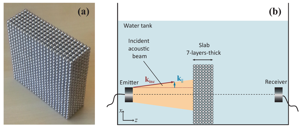
Figure 1.
(a) the finite three-dimensional (3D) sc structure made of touching magnetic spheres of diameter , with dimensions , before its immersion in water; and (b) schematic representation of the experimental setup. The emitter-beam angular spreading (shaded region) is characterized by a wavevector component parallel to the (001) surface of the slab, , varying from zero (normal incidence) to a maximum value depending on frequency.
To analyze the frequency response of this structure, a standard underwater transmission measurement technique is used in the first stage. The corresponding experimental setup is shown in Figure 1b. The sample is immersed in water and placed at the bottom of a sufficiently big water tank to optimally delay side-wall reflections. Both emitting and receiving transducers are broadband -centered Panametrics immersion transducers ( diameter) (Panametrics, Tokyo, Japan). Each one is located at from the (001) surface side of the sample, their mean-beam axis passing at the center of the slab and coinciding with the z-axis, i.e., the incidence is, apart from a symmetric angular spreading, assumed to be in the first order normal to the (001) surface. The emitter transducer is excited by a 5058PR Olympus pulse generator/receiver (Olympus, Tokyo, Japan), providing a high and wide electric pulse. The generator acts also as a trigger for a Yokogawa Numeric Oscilloscope (Yokogawa, Tokyo, Japan) recording signals measured by the receiver transducer and amplified by the 5058PR. The transmitted signals, sampled at and captured within a duration window, are next averaged using 512 acquisitions in order to minimize noise.
The ratio between the Fast Fourier transforms (using eventually zero-padded data in order to decrease the Fourier transform frequency step, and consequently increase the accuracy of the obtained spectra) of the signal transmitted through the slab and the signal transmitted without the slab, i.e., directly from the emitter transducer to the receiver, is formed to obtain a pseudo-transmission coefficient. The corresponding experimental transmittance spectrum is presented in Figure 2a. One observes three pass-band frequency regions separated by relatively large forbidden bands (transmission-gaps) extending from to , from to , and from to , these limits are found if a transmittance level is imposed. These are, in general, in accordance with multiple-scattering theoretical predictions [22], shown in Figure 2b. In the theoretical calculations, the sc (001) planes extend to infinity and a longitudinal acoustic plane wave is considered to be incident normally () on the structure. The main difference when comparing the plots (a) and (b) of Figure 2 is the absence of well constructed Fabry–Perot (FP) resonances in the experimental spectrum within the first transmission band extending up to . Additionally, the experimental gaps are slightly narrower and the whole transmittance spectrum is slightly shifted towards higher frequencies, with the first and second transmission bands leaking within the gap regions, as predicted from the theoretical calculations at normal incidence (Figure 2b). A possible explanation could be the simultaneous generation of several incident waves with different components and amplitudes, due to the angular spreading of the emitter transducer beam, as schematically displayed in Figure 1b. An attempt to reproduce this behavior, theoretically, is given in Figure 2c. We sum the transmittances corresponding to several components along the direction, precisely over , where q varies from 0 to with a step of . Next, we normalize the total-sum curve with respect to its maximum value within the frequency window of interest. The obtained curve mimics quite successfully the behavior of the experimental spectrum at the edges of the two first transmission-gaps. As we move towards higher frequencies, the effect of the transducer-beam angular spreading should weaken, the angular spreading being proportional to the emitted wavelength. This approach does not constitute of course a rigorous proof, especially that the sum should be performed by integrating over the whole irreducible part of the surface Brillouin zone (see Figure 3). Here, we used for simplicity only a part of the direction to match the upper frequency limit of the first transmission band. A complete picture of the transmittance along the whole direction is given in Figure 3.
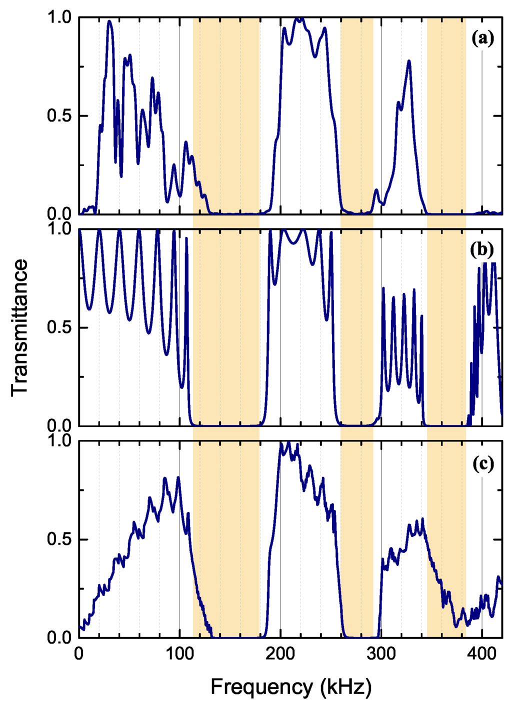
Figure 2.
(a) measured transmittance of an acoustic beam incident on the seven-(001)-layers thick slab of the 3D sc crystal immersed in water; (b) calculated transmittance of a longitudinal plane wave incident normally () on the structure; and (c) normalized sum of the calculated transmittances over several components, with q varying from 0 to with a step of . Shaded regions show gap positions for (b) to guide the eye.
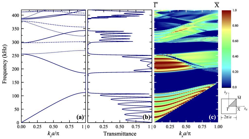
Figure 3.
(a) calculated frequency band structure for the 3D cubic crystal of touching D5N35 spheres (lattice parameter ), immersed in water, along the direction [001] (). Solid, dotted and dashed lines denote, respectively, active non-degenerate bands (symmetry ), inactive non-degenerate bands (symmetry , , ) and inactive double degenerate bands (symmetry ); (b) the corresponding transmittance of a longitudinal plane wave incident normally on a seven-(001)-layers thick slab of the crystal; and (c) color map of the transmittance spectra along the direction () of the surface Brillouin zone shown in the margin.
For a deeper understanding of the behavior of this 3D system and of the origin of the transmission-bands, we calculate the frequency band structure for the sc crystal along the [001] direction (we consider a (001) plane to be the unit cell for the infinite structure and put ). The results are displayed in Figure 3a together with the calculated transmittance of a normally incident plane acoustic wave through a finite slab of seven (001) planes of spheres (see Figure 3b), the same curve as the one of Figure 2b to facilitate comparison. The analysis of the band structure reveals some active bands of symmetry , which represent modes that couple with an external acoustic plane wave, incident normally on a finite (001) slab of the crystal; indeed, perfect agreement exists between these bands and the corresponding transmittance. Additionally, we observe the existence of several inactive (deaf) bands, of symmetry , , , and , which represent modes that do not couple with the above-mentioned external wave incident on the same finite slab. These bands transform into active ones (though, usually, with a weak transmission level) at off-normal incidence (). The first two gaps are Bragg gaps and vary slightly along (see Figure 3c); the third one, around , is a hybridization (or avoided-crossing) gap originating from the existence of some localized modes at this frequency region for the system under study and closes quickly along (see Figure 3c). The role of the symmetry of these bands will become clearer in the following.
As a first remark, we can say that the magnetic character of the spheres does not seem to influence their elastic behavior, as described by the classical theory of elasticity used in the calculation method. The magnetic force which keeps spheres in contact, is not apparent when the experimental results are compared to the corresponding calculations, at least at these frequency scales and with the given degree of accuracy in the obtained spectra. The next step is to study closer the elastodynamic properties of a single sc (001) layer of spheres (i.e., a square array) for two principal reasons. First, the plane, being the unit cell of the 3D crystal, contains by its own, some fundamental properties useful for the analysis of the behaviour of the structure. Often, localized resonances have their origin in the single plane or in the single sphere, whose separate study can illuminate the physical origin of the phenomena. Second, such a plane can offer a lower-dimension structure than the corresponding 3D case. In addition, the question to answer is: does the main conclusion of this part concerning the magnetic character of the spheres still remain valid? For these reasons, we will focus next on the corresponding 2D case: a single sc (001) plane of touching magnetic spheres, immersed in water.
3.1.2. Two-Dimensional Structure
In this part, we present some experiments concerning the single square array of touching D5N35 spheres (lattice constant ), immersed in water, together with the theoretical analysis of the underlying physical mechanisms. Precisely, two different experiments have been realized: transmission at normal incidence and guided-wave detection, both involving the same transducers, electronics and time signal processing, as for the case of the measured, at normal incidence, transmittance through the slab of the 3D crystal of spheres.
We begin with the study of the transmission properties of the monolayer of spheres. We compute the corresponding transmittance of an acoustic plane wave through the array for the case of normal incidence (). The results are shown in Figure 4a. We observe a transmission resonance peak at , which corresponds to the first FP resonance of an equivalent homogeneous fluid plate of effective thickness D and whose effective elastic parameters, mass density and longitudinal propagation velocity , can be estimated as follows. Applying theoretical developments for disordered arrays of spherical particles, with a 3D spatial distribution, embedded in a host medium [30], for the case of the 3D sc crystal with , the volume filling fraction occupied by the spheres, we find that the crystal can be described, at the long-wavelength limit, by an equivalent effective medium with parameters and . The latter is in very good agreement with the corresponding slope, as calculated from the band structure diagram () given in Figure 3a. However, we expect that when the dimensions of the system become lower, going from the 3D cubic crystal to the single 2D square array, the assumption of isotropic 3D spatial distribution of the spheres is not valid anymore and these effective parameters cannot describe the behaviour of the array at low frequencies. We calculate the transmittance of an acoustic plane wave through a fluid plate of thickness and with elastic parameters and (dashed line in Figure 4a), where the thickness has been adjusted in order to produce the FP at the same frequency position (). Of course, the pair (D,) is not unique. For instance, putting and (i.e., with constant ) reproduces perfectly the low-frequency behaviour of the array, with only a slight adjustment of (dotted line in Figure 4a). At higher than the FP frequencies, this effective picture fails to describe the response of the composite layer. Other phenomena such as resonances originating from the spheres and/or lattice effects will appear, giving a more complex structure in the calculated transmittance of the square array. We observe some prominent peaks at and and two clear dips at and , which occur slightly below the cut-off frequencies for the generation of the first two non-zero orders of the diffracted beams, and (corresponding to reciprocal-lattice vectors , i.e., with , and , i.e., with , respectively). These dips are, in other words, associated to lattice resonances, localized in the plane passing at the center of the spheres, the first of them corresponding to the first lattice resonance along , i.e., with wavelength , and the second to the first lattice resonance along , i.e., with wavelength . The same phenomenology has been observed for monolayers of solid spherical particles embedded in a solid matrix [31].
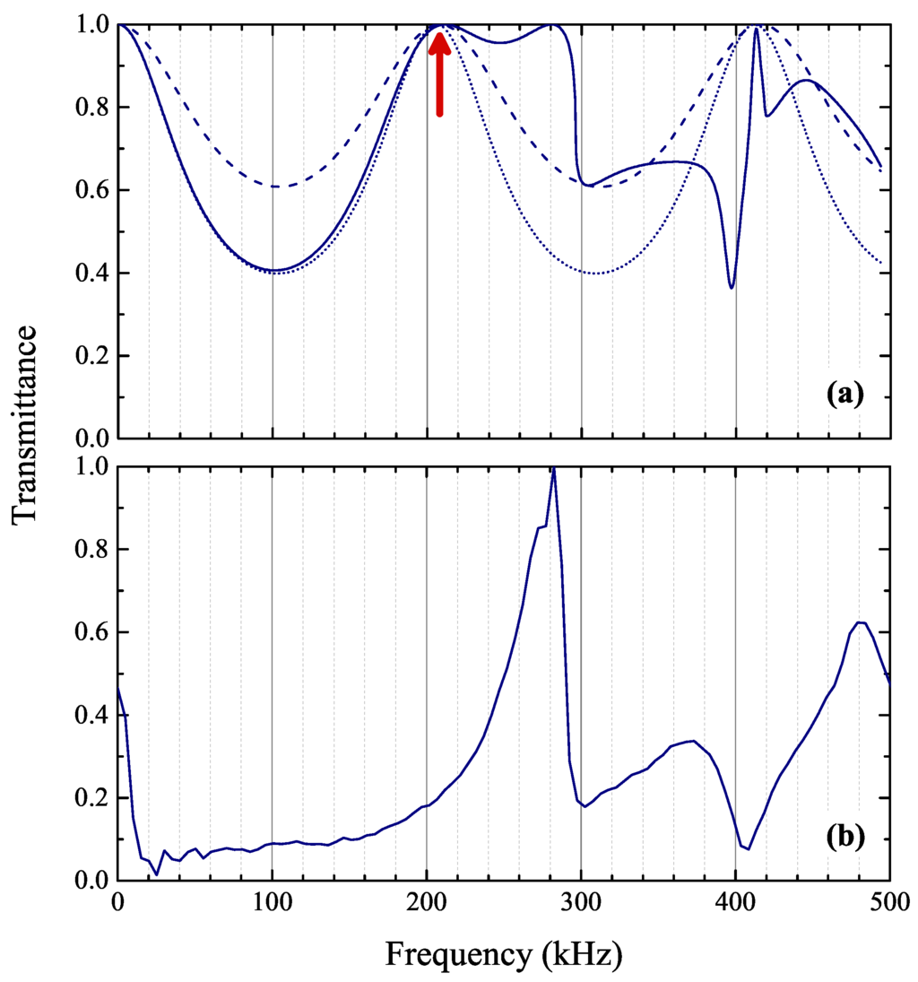
Figure 4.
(a) calculated transmittance (solid line) of a plane acoustic wave through a (001) layer of D5N35 touching spheres (), immersed in water. With dashed (dotted) line we show the calculated transmittance of such a wave through an effective, homogeneous fluid plate of thickness () with elastic parameters () and (). The red arrow indicates the position of the first FP resonance; and (b) the corresponding measured transmitted pressure of a (001) layer of spheres excited by an immersion transducer beam.
Following the same experimental procedure as that described in the previous section, we obtain the transmitted pressure through a sc (001) plane of spheres excited by the transducer’s acoustic central beam incident normally on the plane. The results, normalized to their maximum value in the frequency window , are plotted in Figure 4b. Apart from the low frequency region (i.e., below ) where the transducers sensibility vanishes, most of the features predicted by the theoretical curve are present. We observe a sharp transition about 280–300 and a transmission dip at . The main difference seems to be the absence of the FP peak at about . In fact, the very strong narrow peak at obscures the FP resonance that is hidden in the background. We verified this hypothesis by calculating the transmitted pressure through the square array, where the FP peak is found to be relatively weakened in amplitude, in accordance with the picture obtained experimentally.
Next, we focus on the study of the guided wave response of the monolayer. We proceed to its experimental characterization by measuring the transmitted pressure through the layer, adopting for the transducers a transmission configuration, as the one shown in Figure 5a, i.e., with their axis making an angle of with the normal to the plane, in order to probe elastic modes propagating along the layer and being localized in it with respect to the z-direction. We note in passing that the choice of the angle ensures that guided waves will be excited and thus observed in the frequency region of interest, without completely losing the symmetry advantages of the normal incidence. Both transducers’ mean beams belong to the same plane as the normal to the plane; the projection of the wavevector component parallel to the layer lies on the direction of the surface Brillouin zone (see inset of Figure 3), , q varying from 0 to . The receiver is translated parallel to the layer (x-axis), and the pressure scattered by the plate is captured every , from to (we set at the location of maximal forced transmission regime). After a double time-space FFT in the free time and space regime of the signal, we obtain the transmitted pressure in the frequency-wavenumber space, , whose modulus is plotted in Figure 5b. We observe a more or less continuous transmission band of relatively weak amplitude, extending up to ∼300 , interrupted by two transmission-gap regions, from 140 to and from 225 to . This physical picture is in accordance with the one shown in the transmission plot along direction (Figure 3c), for . The nature of these modes is of FP type; in this frequency region, i.e., below , no localized modes exist originating from the spheres or from one plane of spheres, and the behaviour of the real system is practically the same to that of an array of rigid (impenetrable) scatterers. Acoustic waves hardly penetrate within the sphere and its interior is not seen. The most important feature of the guided-response plot of Figure 5b is the appearance of three isolated, well-defined, and relatively high-amplitude spots centered at 308, 394, and . We note here that the peak level of the second spot (the strongest one) has been saturated in order to better visualize the two others.
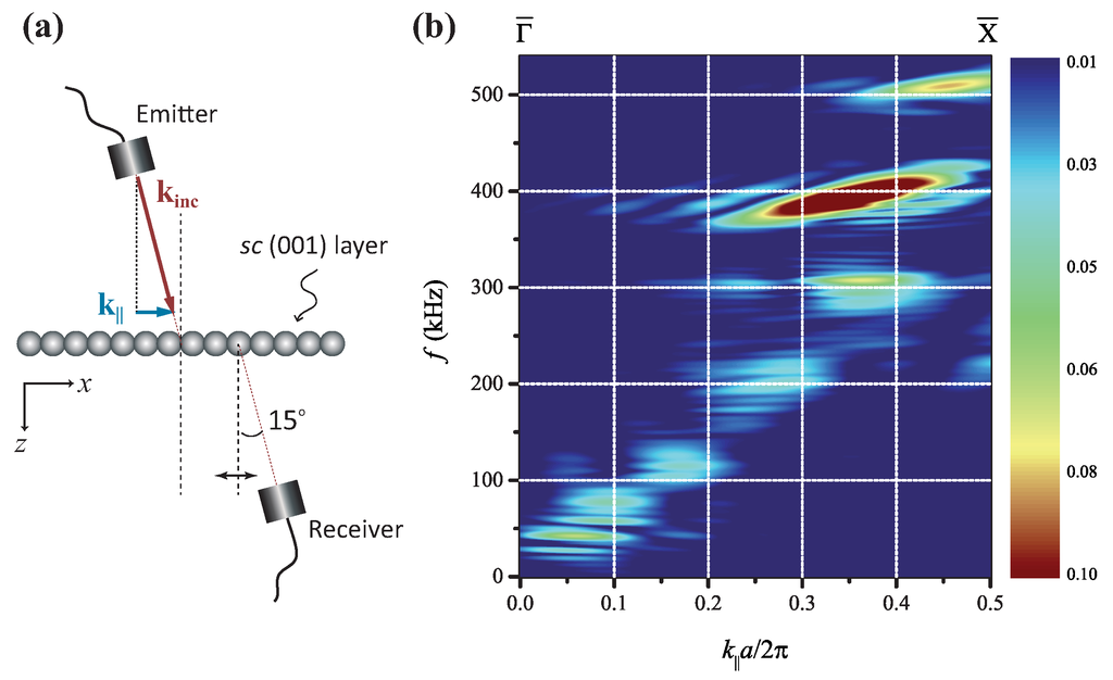
Figure 5.
(a) schematic representation of the transmission configuration used to measure the guided wave response of the square monolayer of spheres. The incident and transmitted central beam axes lie on a plane containing the normal to the monolayer; the wavevector component parallel to the layer, , is along the direction of the square array; and (b) the modulus of the space-time (x-t) Fourier transform of the pressure transmitted in the free guided regime along the x-direction, plotted versus the reduced wavevector along the direction.
In order to clarify the origin of these three observed peaks, we need to analyze theoretically the resonant behaviour of one single sphere and of a square-array monolayer of such touching spheres. In Figure 6a, we show the calculated change in the density-of-states of the elastic field (Equation (5)) for a D5N35 sphere () immersed in water, with respect to the infinitely extended water. In the frequency window that interests us here, , there is only an (quadrupole-like) five-fold spheroidal mode at about , manifested as a Lorentzian-shape peak in the DOS spectrum and whose elastic field spatial distribution (see inset plot in Figure 6a) reveals a -like orbital form corresponding to angular momentum numbers. When bringing spheres close to form a 2D square array of spheres, the high, spherical symmetry of the system lowers, and we expect that the five-fold degeneracy (, for ) splits up to five non-degenerated modes. Indeed, for a lying, for instance, on the direction, we obtain five non-degenerate modes, corresponding to five Lorentzian peaks, each of them of different height and width, as shown in Figure 6b for , through DOS calculations for the monolayer (Equations (5) and (6)).
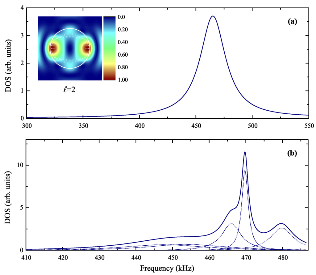
Figure 6.
(a) calculated difference in the density-of-states of the elastic field for a D5N35 sphere (diameter ) immersed in water, with respect to the infinitely extended host medium (water), revealing an five-fold resonant mode. In the inset, we give, after extraction of the incident component, the color map of the modulus of the elastic field at resonance (), in a plane passing at the center of the sphere (incidence is assumed along the horizontal axis directed from left to right); the white arrows show the direction of the elastic field; and (b) calculated difference in the density-of-states of the elastic field for a square array of touching D5N35 spheres (diameter ) immersed in water, with respect to the infinitely extended host medium (water) for , revealing the splitting of the five-fold resonant modes of the individual sphere to five non-degenerate modes (dotted lines).
The physical meaning of these modes can become clearer if we go back to a high-symmetry point in the -space. Following group theory basic arguments, we can show [32] that an , five-fold, spherical mode at the Γ point, , splits into a double-degenerated mode of symmetry and a triple-degenerated mode of symmetry . Considering now along the [001] direction, lowers further the symmetry of the system to the symmetry, and these modes split as and . In other words, flat localized bands originating from an resonant mode of the sphere will split along the [001] direction to three non-degenerate bands of symmetry , , and and one double-degenerate band of symmetry . We remember, at this point, the connection between these symmetries and the d-orbitals. transforms like a orbital (angular momentum numbers , ), and it has a spatial distribution along the z-axis, perpendicular to the (001) plane of spheres. This mode couples with a longitudinal wave incident normally on the plane. and transform like and orbitals (, ), respectively, lying both on the -plane. The former has its lobes aligned along x- and y-axes and can thus be excited by a incident wave with a component along the direction; the latter has its lobes aligned along the lines and can thus be excited by an incident wave with a component along direction. Finally, transforms like a or orbital (, ), both having their lobes on the planes and at with respect to the z-axis. From the above, it is thus evident that only modes with symmetry will be localized on the (001) plane along the direction. After analysis of the eigenmodes for the band structure of Figure 3a, we find that there exists a flat mode of symmetry at about originating from the mode of the individual sphere. This mode corresponds to the one bright experimental spot at .
The other two bright experimental spots, at 308 and , do not originate from resonant modes of the individual sphere. They correspond to lattice resonances, and both of them constitute the evolution with of the first dip at about , observed in the transmission spectrum of the monolayer at normal incidence () shown in Figure 4a. We remember that this dip is associated with a lattice resonance corresponding to reciprocal lattice vectors with . The dispersion relation of these lattice resonances can be approximately described by setting the z-component of the wavevector (Equation (1)) equal to zero, i.e., . For lying along , , and we have . The first bright spot, at , is very close to the value of obtained from this dispersion relation for and . In other words, this spot corresponds to the first lattice resonances along and whose dispersion relation varies very little with along . Of course, this double-degenerated mode, lying outside should not be observed; however, it produces a weak spot due to some angular spreading of the emitter transducer, thus exciting slightly modes out of the . The second bright spot, at , is very close to the value of obtained from this dispersion relation for and . In other words, this spot corresponds to the first lattice resonance along and its dispersion relation varies significantly with along . This mode produces a high-amplitude spot since the corresponding lattice resonance is naturally aligned along . We note in passing that, following similar analysis, close to the third experimental spot at about , there exists a branch corresponding to a lattice resonance: for , we obtain , which could probably interfere with the mode originating from the sphere resonance.
3.2. Linear Chain Immersed in Air
We close this study by considering a 1D periodic array, a linear chain with lattice constant a, composed of N touching magnetic spheres of diameter . An example of the fabricated samples used in the experiments, is shown in Figure 7a, together with the experimental setup. The chain is placed horizontally onto a PVC substrate in order to facilitate the positioning of the experimental apparatus and ensure the straight alignment of the chain.
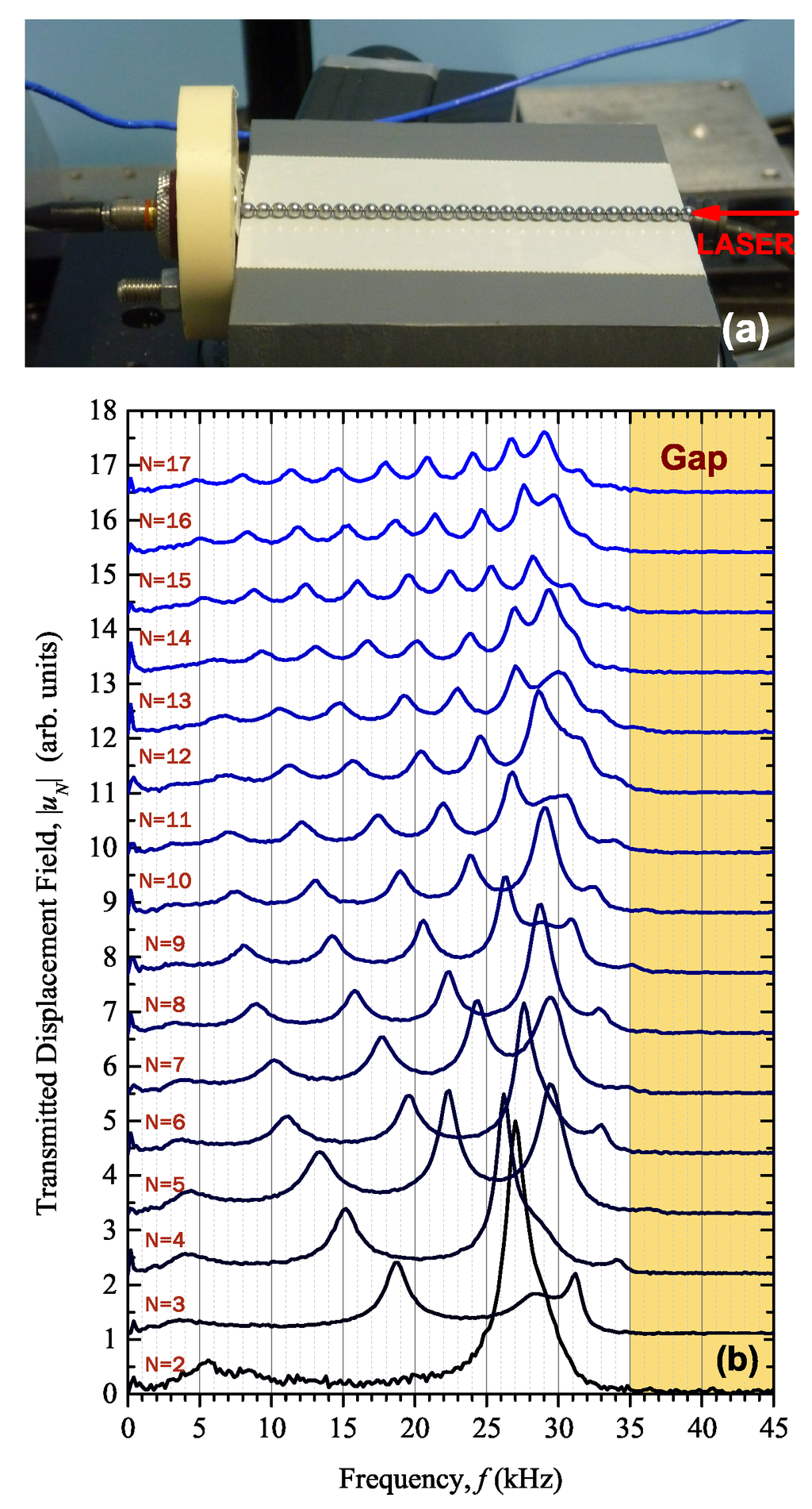
Figure 7.
(a) chain of N metallic spheres of diameter , excited by a longitudinal transducer (left) with the transmitted signal recorded at the end of the chain through LDV (right); (b) the modulus of the transmitted displacement field measured at the end of the chain, , as a function of frequency f, for various chain lengths, . The different spectra are displaced vertically to improve visibility.
A broadband longitudinal wave contact transducer is put in contact with the spherical bead located at one extremity of the chain, the axes of the transducer and the linear chain being identical. The transducer (Panametrics, Tokyo, Japan), central frequency: , diameter: ), acting as an emitter, is plugged to a Sofranel high voltage pulser/receiver (Sartrouville, France) delivering a high and wide pulse. An OFV-505 Polytec laser velocimeter (Waldbronn, Germany) is used to measure the normal displacement at the end of the chain: the laser beam of the velocimeter is reflected at normal incidence at the point diametrically opposite to the contact point of the chain with the transducer. The elastic response of the chain provided by the velocimeter is recorded by a 12-bit hro 66zi Teledyne LeCroy oscilloscope (New York, NY, USA) over a time window at sampling frequency. The fast Fourier transform (FFT) is processed “as is” on the signal recorded for each chain, revealing two well separated frequency regions with distinct response: a low-frequency region below ∼100 and a high-frequency region beyond ∼400 . In all cases discussed here, the horizontally aligned, normal to the surface of the sphere, component of the elastic field, , is thus obtained, as a function of frequency f. We study several chain lengths, , for three different sphere types, D10N40, D5N35 and D3N42 (see Table 1).
3.2.1. Low-Frequency Response
The experimentally obtained transmitted elastic field at the end of the chain, , in the low (kHz-range) frequency region is presented in Figure 7b, for chain lengths varying from 3 to 18 D5N35 beads (). One observes a Fabry–Perot (FP) type pass-band extending up to characterized by an, increasing with N, number of FP resonance peaks; the band is followed by a transmission-gap (shaded region in Figure 7b).
The phase of the previous FFT signal transmitted through a sufficiently long chain of length , when plotted as a function of frequency f, can provide an experimental dispersion relation. In Figure 8a, we plot (solid line) the normalized phase after averaging for chains from to 18-beads long in order to minimize residual fluctuations in the plot. The result is in accordance with the pairs where , , some discrete wavenumbers (open symbols in Figure 8a) associated to the frequency positions of the FP peaks, , in the corresponding displacement field spectrum for a finite chain made of spheres (Figure 8b). This discrete wavenumber rule is based on a simple physical picture, taking into account the specific boundary conditions applied for the longitudinal displacement field at both ends of the finite chain, as schematically shown in Figure 8c. Following this picture, one should write that the FP resonances must occur when , where . The two methods described above to obtain the experimental dispersion plot, i.e., the phase-deduced band structure and the FP-based discrete model, should be in good agreement for sufficiently long chains, at least for the lower frequency bands; and this is indeed the case here. As a guide to the eye and to facilitate the comparison, we plot a smoothed curve passing at the points (see dotted line in Figure 8a). Again, a transmission-gap region is confirmed, with lower frequency limit at , in accordance with the conclusions drawn when studying the transmission spectra (see Figure 7).

Figure 8.
(a) experimental dispersion plot of a linear chain of lattice parameter a, made of N touching spheres (diameter ) deduced from the FFT phase (solid line) compared to a discrete model description represented by the pairs with (open symbols). The dotted line is a non-linear interpolation connecting the discrete points , revealing a clear propagative band ranging from 0 to ; (b) experimental transmitted displacement field spectrum for the case of a finite chain (). Horizontal dashed lines are guides to the eye, associating the frequency positions of the FP resonance peaks, , to the discrete wavenumbers , for the case of spheres (see text); (c) a schematic representation of the FP resonances in the linear chain configuration with open-closed boundary conditions applied at the extremities of the chain.
However, the most important characteristic is the linear dispersion at the long-wavelength limit (), allowing for the determination of the effective medium slope, which is found to be . This result does not agree with calculations based on multiple-scattering techniques [28] extended here to include the case of an infinite chain of metallic beads immersed in air. The theoretical dispersion relation gives, at , an effective medium propagation velocity . This discrepancy is related to the existence of the magnetic force between spheres producing a weak Hertzian contact. The radius of the circular-shaped contact region, β, is calculated from the relation (A2) given in Appendix A to be of the order of of the sphere’s radius (see Table 1), where and are the Poisson ratio and the Young modulus of the magnetic alloy, respectively, obtained from the values of Table 2. The dispersion plot based on the above discrete picture (dotted line in Figure 8a) is in very good agreement with a mass-spring monatomic linear chain model providing the relation , being the cut-off frequency of the acoustic branch and (see Appendix A). Following this description, we obtain after non-linear fitting an effective velocity and a cut-off frequency .
The deviation of the experimental band structure (solid line, Figure 8a) from the simple discrete developed model (dotted line, Figure 8a) at the region of the gap is due to finite-size effects and some attenuation in air. Beyond the gap region, no higher-order propagative effective medium bands are observed, as expected from a monatomic chain image. We also note here that, in the low-frequency region, the chosen combination of materials (metallic spheres in air) follows the typical behavior of a rigid-scatterer assembly and does not exhibit any resonances originating from the individual sphere. These are expected to appear at about , where d is the diameter of the sphere expressed in meters, as predicted from DOS calculations (see also Figure 6a).
The same analysis is repeated for a chain made of D3N42 spheres. The results, following the same methodology, are presented in Figure 9. Again, the FP resonance peaks in the spectrum of the transmitted field (we consider the case of a chain with spheres), shown in Figure 9b, in conjunction with the discrete wavenumber model provide a set of pairs which, after interpolation (dotted line in Figure 9a), compare well with the normalized-phase curve (solid line in Figure 9a). As previously, we obtain at the long-wavelength limit an effective-medium velocity = 456 ; the cut-off frequency is at about . The main difference, however, with the previously studied case (D5N35 spheres) is the existence of a pronounced dip in the transmission spectrum around , corresponding to an S-like form in the dispersion plot (a qualitative explanation is given in Appendix A). This is the fingerprint of an avoided-crossing gap originating from the interaction of the first longitudinal waveguide mode of the PVC substrate with the effective-medium propagating band. Indeed, for a -thick PVC plate, whose elastic parameters are shown in Table 2, the first FP resonance occurs at . Finally, this dispersion plot (dotted line in Figure 9a) can be described by the mass-spring monatomic linear chain model ; we obtain after non-linear fitting an effective velocity and a cut-off frequency .
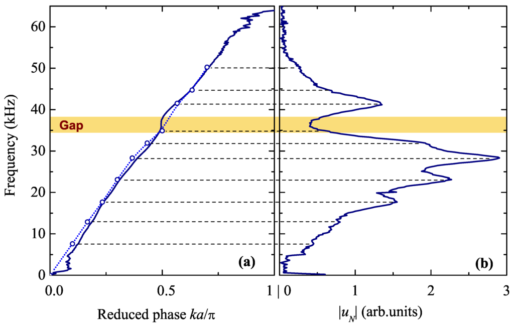
Figure 9.
(a) experimental dispersion plot of a linear chain of lattice parameter a, made of N touching spheres (diameter ); (b) experimental transmitted displacement field spectrum for the case of a finite chain (). All symbols, methods and analysis follow the same scheme as the one used in Figure 8.
Similar results were obtained for a chain made of bigger spheres (D10N40). The effective medium slope has been found to be . The values for the effective-medium velocity together with the radius of the contact area (see Equation (A2) of Appendix A) are summarized, for all samples studied, in Table 1. Knowledge of can be used to extract the power law relating the effective propagation velocity to the applied force. With the help of Equations (A9) and (A10) and if we set to be the same for all samples, we calculate the exponent n to be close to six (see Table 1), this specific value characterizing a Hertz-type elastic contact. We note that a different power law () has been recently observed for the same kind of spheres, without variation of the diameter [20].
The low-frequency study concludes the following remarks. Two main differences are to be noted between the 1D configuration and the two previous cases (2D and 3D phononic crystals). First, the 1D array is immersed in air instead of water, and second, the excitation of the system is realized through contact of the transducer directly with the solid material of the spheres. These two points mean that we can neglect, at a first approximation, the existence of air in our analysis. The 1D system should behave like a periodically corrugated cylindrical waveguide, since the spheres are in elastic contact, forming a continuous network. Multiple-scattering calculations fail to describe, in this case, the dispersion relation of the longitudinal mode, along the chain, since the scattering is considered to take place in the air region and not in the interior of the spheres. When chains, made of rare earth magnetic spheres, are excited by contact transducers (i.e., propagation and scattering take place mainly in the material of the spheres), the system behaves as predicted by Hertz’s theory of elastic contact, at least for weak applied static forces of the order of GPa. When 2D and 3D periodic structures made of magnetic spheres in contact are immersed in water, the excitation process (and subsequently the scattering of acoustic waves) is realized in the water region; the elastic contact does not produce an observable effect, as compared to multiple-scattering calculations, which do not take into account in any case the elastic contact between spheres.
3.2.2. High-Frequency Response
As expected from the linear chain image, described previously, no higher propagative bands exist beyond the cut-off frequency of the acoustic branch. However, at higher frequencies (MHz-range), localized flat resonant modes are expected to appear; they propagate along the chain, originating from the corresponding resonances of the individual sphere. For a chain made of spheres with , we experimentally observe the formation of narrow, high-amplitude resonant bands around the and resonances of spheroidal modes of the individual sphere, as confirmed by DOS calculations and a multipole mode analysis for the system [22,28]. These bands are centered at and , respectively, as shown in the left panel of Figure 10; the theoretical calculation (right panel of Figure 10) predicts and , for the individual sphere, if the elastic parameters of Table 1 are used. Similar results are found for chains made of D5N35 and D10N42 spheres, confirming this high-frequency-response image.
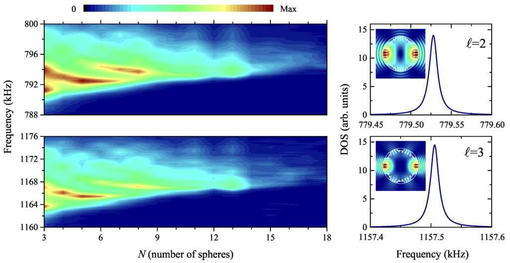
Figure 10.
(left): color map of the transmitted displacement field measured at the end of a chain made of N D3N42 magnetic spheres (), as a function of frequency and number of spheres. Two narrow localized bands are observed, originating from (top) and (bottom) resonance modes of the individual sphere; (right), the corresponding DOS calculations for one sphere, together with the elastic field on resonance, at a cut passing at the center of the sphere (incidence is considered from left to right).
4. Conclusions
In the present paper, we studied experimentally the elastic response of 1D, 2D and 3D phononic crystals, made of rare-earth magnetic spheres in contact, immersed in a fluid (air for the 1D and water for the 2D and 3D structures). The excitation process (immersion or contact transducers) has been shown to differentiate the behavior of the system, regarding the influence of the elastic contact between adjacent spheres on the obtained dispersion relation of the structures. In particular, we have shown that, although the magnetic force is present in all cases, producing the contact between spheres that form a close solid network, its effect seems to vanish when excitation takes place in the immersion fluid (water), while it cannot be neglected when excitation takes place in the magnetic material (the immersion fluid is air). Our experimental results have been successfully compared to theoretical predictions using multiple-scattering techniques, in the first case. The multiple-scattering description fails. In the second case, Hertz contact cannot be neglected. The structures considered here are easy to fabricate, since they do not necessitate any adhesion treatment and their technique of construction is non-destructive. They can be ideal candidates for practical applications where one needs to use phononic structures immersed in a fluid host medium and are shown to exhibit interesting properties as narrow frequency filters in the case of 1D arrays. Their study, from a theoretical point of view, is also of interest, especially in the case of several elastic or plastic contact models.
Author Contributions
All authors conceived, designed and performed the experiments; Pascal Rembert and Rebecca Sainidou performed the theoretical calculations, analyzed the data, and wrote the paper.
Conflicts of Interest
The authors declare no conflict of interest.
Abbreviations
The following abbreviations are used in this manuscript:
| 1D | one-dimensional |
| 2D | two-dimensional |
| 3D | three-dimensional |
| FP | Fabry–Perot |
| DOS | density of states |
| FFT | fast Fourier transform |
| LDV | laser Doppler vibrometer |
| LMS | layer multiple scattering |
Appendix A
We assume two identical elastic spheres of diameter d, made of the same material that is characterized by a mass density ρ, Poisson ratio ν and Young modulus E. The two spheres are in contact with a mutual compressive static force, , applied between each other along the line connecting their centers; this force transforms the point contact to a circular-shaped area of radius β and the center-to-center distance decreases by δ, the indentation depth, as schematically depicted in Figure A1. For δ small enough as compared to the diameter d, following Hertz’s theory of elastic contact [33], we can calculate the indentation depth
and the radius of the contact area
expressed as functions of the compressive applied force [34]. We note here that the applied force scales as ∼, this non-linear, power-law relation being only a purely geometrical effect: linear elasticity is considered. Combining Equations (A1) and (A2), we obtain the following useful relation:
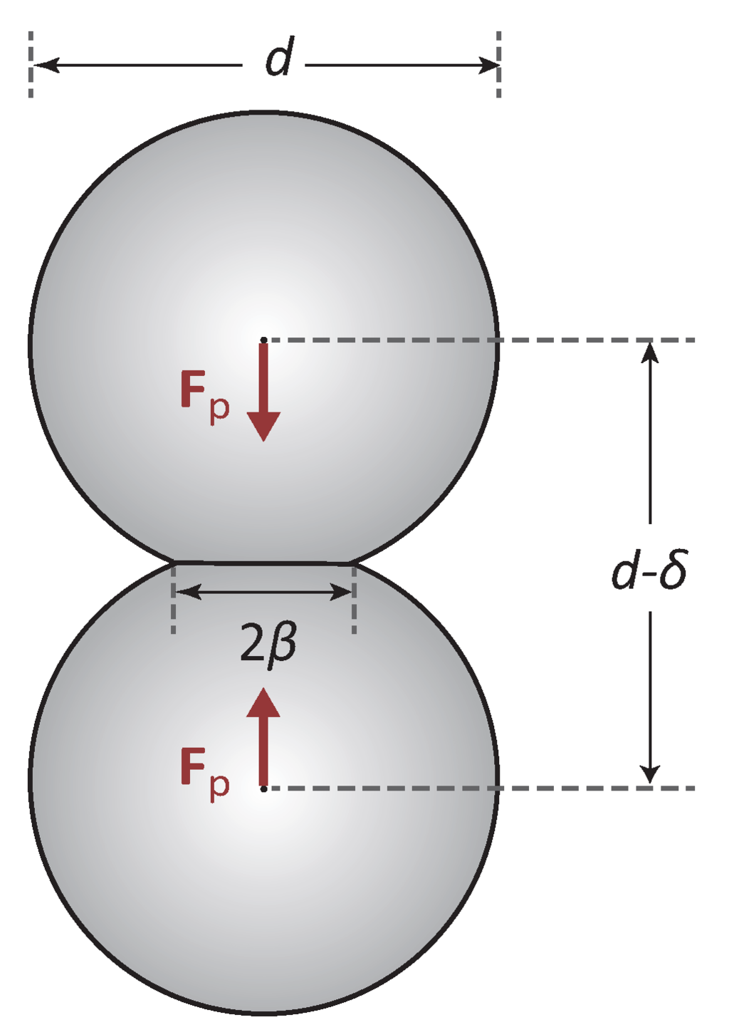
Figure A1.
geometry of the problem of two elastic spheres in contact under the action of an applied compressive force.
For and (see Table 2), we compute β and δ to be, respectively, of the order of and of the sphere’s radius, in all cases.
The relation (A1) written appropriately allows for the determination of the effective contact stiffness K defined as . We find
A linear chain of identical spheres in Hertzian contact can be described in the linear regime as a mass-spring periodic array of lattice constant , the masses being those of the spheres, i.e., , and the springs having stiffness K given by (A4). The dispersion relation of such a chain is
where is the cut-off frequency denoting the upper frequency limit of the acoustic branch (see Figure A2a) beyond which no modes exist (gap region extending to infinity). The cut-off frequency is related to a chain’s characteristics through the relation
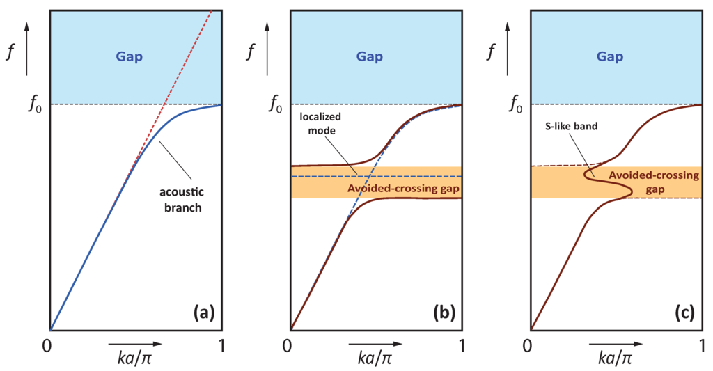
Figure A2.
(a) schematic representation of the dispersion relation for a periodic mass-spring array of lattice constant a. The acoustic branch (solid line) is perfectly described, at the long-wavelength limit, by a linear dispersion corresponding to an effective-medium propagation velocity (broken line), while the cut-off frequency delimits the lower frequency limit of the extended to infinity band gap (shaded area); (b) as in (a) but with the presence of a localized flat mode which, after interaction with the acoustic branch of the chain’s dispersion relation, gives rise to an avoided-crossing gap (shaded area) below the cut-off frequency. Broken lines: the bands before hybridization; (c) modification of the dispersion plot shown in (b) when absorption is taken into account (see text) leading to an S-like band within the avoided-gap region, which corresponds to modes with complex wavenumber.
The dispersion relation (A5) is linear at the long-wavelength limit (dotted line in Figure A2a) corresponding to a constant with frequency effective-medium velocity
This last equation should describe the long-wavelength limit behaviour of a linear chain of touching spheres under a static applied force generating a Hertz-type elastic contact between adjacent spheres. We can then write
where
in the case of Hertz contact, as it turns out after comparison to Equation (A8). Equations (A9) and (A10) are of practical importance, when is deduced from the experimental results (as is the case here) in order to confirm or reject a Hertz-type contact.
Finally, a last comment on the possible variants of the form that the dispersion plot can take, worth pointing out at this point. We expect that a chain of touching spheres with elastic contact between them due to an applied static force would present, in a good approximation, a dispersion plot as the one shown schematically in Figure A2a. In practice, some deviations from this form can also occur, such as the appearance of an avoided-crossing gap, after hybridization between the acoustic branch mode and some flat localized mode. The latter originates from some resonances of the scatterers (spheres) or even from those of a substrate used to support the chain. This is indeed the case encountered here: the acoustic-branch frequency region is free of resonances localized in the spheres, the first of them occurring at about ∼230 for magnetic spheres of diameter , but there are some originating from the PVC substrate. Precisely, the first FP resonance occurs at about and will therefore be visible in the acoustic branch region as schematically presented in Figure A2b. When absorption is present in the system, this avoided-crossing gap will transform to an S-like band (see Figure A2c) whose elastic modes exhibit a Bloch wavevector with a small non-zero imaginary part; an analog is observed in the case of surface plasmons polaritons at a metal/insulator interface [35].
References
- Khelif, A.; Adibi, A. Phononic Crystals: Fundamentals and Applications; Springer Science + Business Media: New York, NY, USA, 2016. [Google Scholar]
- Deymier, P. (Ed.) Acoustic Metamaterials and Phononic Crystals. In Springer Series in Solid-State Sciences; Springer-Verlag: Berlin, Germany; Heidelberg, Germany, 2013.
- Farhat, M.; Enoch, S.; Guenneau, S.; Movchan, A.B. Broadband Cylindrical Acoustic Cloak for Linear Surface Waves in a Fluid. Phys. Rev. Lett. 2008, 101, 134501. [Google Scholar] [CrossRef] [PubMed]
- Yang, S.; Page, J.H.; Liu, Z.; Cowan, M.L.; Chan, C.T.; Sheng, P. Focusing of Sound in a 3D Phononic Crystal. Phys. Rev. Lett. 2004, 93, 024301. [Google Scholar] [CrossRef] [PubMed]
- Maldovan, M. Sound and heat revolutions in phononics. Nature 2013, 503, 209–217. [Google Scholar] [CrossRef] [PubMed]
- Addouche, M.; Al-Lethawe, M.A.; Choujaa, A.; Khelif, A. Superlensing effect for surface acoustic waves in a pillar-based phononic crystal with negative refractive index. Appl. Phys. Lett. 2014, 105, 023501. [Google Scholar] [CrossRef]
- Cheng, W.; Wang, J.J.; Jonas, U.; Fytas, G.; Stefanou, N. Observation and tuning of hypersonic bandgaps in colloidal crystals. Nat. Mater. 2006, 5, 830–836. [Google Scholar] [CrossRef] [PubMed]
- Akimov, A.V.; Tanaka, Y.; Pevtsov, A.B.; Kaplan, S.F.; Golubev, V.G.; Tamura, S.; Yakovlev, D.R.; Bayer, M. Hypersonic Modulation of Light in Three-Dimensional Photonic and Phononic Band-Gap Materials. Phys. Rev. Lett. 2008, 101, 033902. [Google Scholar] [CrossRef] [PubMed]
- Alonso-Redondo, E.; Schmitt, M.; Urbach, Z.; Hui, C.M.; Sainidou, R.; Rembert, P.; Matyjaszewski, K.; Bockstaller, M.R.; Fytas, G. A new class of tunable hypersonic phononic crystals based on polymer-tethered colloids. Nat. Commun. 2015, 6, 8309. [Google Scholar] [CrossRef] [PubMed]
- Caleap, M.; Drinkwater, B.W. Acoustically trapped colloidal crystals that are reconfigurable in real time. Proc. Natl. Acad. Sci. USA 2014, 111, 6226–6230. [Google Scholar] [CrossRef] [PubMed]
- Kinra, V.K.; Henderson, B.K.; Maslov, K.I. Elastodynamic response of layers of spherical particles in hexagonal and square periodic arrangements. J. Mech. Phys. Solids 1999, 47, 2147. [Google Scholar] [CrossRef]
- Leroy, V.; Strybulevych, A.; Scanlon, M.G.; Page, J.H. Transmission of ultrasound through a single layer of bubbles. Eur. Phys. J. E 2009, 29, 123–130. [Google Scholar] [CrossRef] [PubMed]
- Johnson, K.L. Contact Mechanics; Cambridge University Press: Cambridge, UK, 1985; pp. 84–106. [Google Scholar]
- Hladky-Hennion, A.-C.; Cohen-Tenoudji, F.; Devos, A.; de Billy, M. On the existence of subresonance generated in a one-dimensional chain of identical spheres. J. Acoust. Soc. Am. 2002, 112, 850–855. [Google Scholar] [CrossRef]
- Coste, C.; Falcon, E.; Fauve, S. Solitary waves in a chain of beads under Hertz contact. Phys. Rev. E 1997, 56, 6104–6117. [Google Scholar]
- Tournat, V.; Gusev, V.E.; Castagnède, B. Self-demodulation of elastic waves in a one-dimensional granular chain. Phys. Rev. E 2004, 70, 056603. [Google Scholar] [CrossRef] [PubMed]
- Daraio, C.; Nesterenko, V.F.; Herbold, E.B.; Jin, S. Tunability of solitary wave properties in one-dimensional strongly nonlinear phononic crystals. Phys. Rev. E 2006, 73, 026610. [Google Scholar] [CrossRef] [PubMed]
- Merkel, A.; Tournat, V.; Gusev, V. Experimental Evidence of Rotational Elastic Waves in Granular Phononic Crystals. Phys. Rev. Lett. 2011, 107, 225502. [Google Scholar] [CrossRef] [PubMed]
- Sanchez-Morcillo, V.J.; Perez-Arjona, I.; Romero-Garcıa, V.; Tournat, V.; Gusev, V.E. Second-harmonic generation for dispersive elastic waves in a discrete granular chain. Phys. Rev. E 2013, 88, 043203. [Google Scholar] [CrossRef] [PubMed]
- Sierra-Valdez, F.J.; Pacheco-Vázquez, F.; Carvente, O.; Malloggi, F.; Cruz-Damas, J.; Rechtman, R.; Ruiz-Suárez, J.C. Acoustic gaps in a chain of magnetic spheres. Phys. Rev. E 2010, 81, 011301. [Google Scholar] [CrossRef] [PubMed]
- Psarobas, I.E.; Stefanou, N.; Modinos, A. Scattering of elastic waves by arrays of spherical bodies. Phys. Rev. B 2000, 62, 278–291. [Google Scholar] [CrossRef]
- Sainidou, R.; Stefanou, N.; Psarobas, I.E.; Modinos, A. A layer-multiple-scattering method for phononic crystals and heterostructures of such. Comput. Phys. Commun. 2005, 166, 197–240. [Google Scholar] [CrossRef]
- Korringa, J. On the calculation of the energy of a Bloch wave in a metal. Physica 1947, 13, 392–400. [Google Scholar] [CrossRef]
- Kohn, W.; Rostoker, N. Solution of the Schrödinger Equation in Periodic Lattices with an Application to Metallic Lithium. Phys. Rev. 1954, 94, 1111–1120. [Google Scholar] [CrossRef]
- Pendry, J.B. Low Energy Electron Diffraction; Academic Press: London, UK, 1974. [Google Scholar]
- Sainidou, R.; Stefanou, N.; Psarobas, I.E.; Modinos, A. The layer-multiple-scattering method applied to phononic crystals. Z. Kristallogr. 2005, 220, 848–858. [Google Scholar] [CrossRef]
- Assouar, B.; Sainidou, R.; Psarobas, I.E. The Three-Dimensional Phononic Crystals. In Phononic Crystals: Fundamentals and Applications; Khelif, A., Adibi, A., Eds.; Springer Science + Business Media: New York, NY, USA, 2016; pp. 51–84. [Google Scholar]
- Sainidou, R.; Stefanou, N.; Modinos, A. Green’s function formalism for phononic crystals. Phys. Rev. B 2004, 69, 064301. [Google Scholar] [CrossRef]
- Dadon, D.; Dariel, M.P.; Gefen, Y.; Klimker, H.; Rosen, M. Low temperature elastic properties of the permanent magnet compound Nd2Fe14B. Appl. Phys. Lett. 1986, 48, 1444–1445. [Google Scholar] [CrossRef]
- Gaunaurd, G.C.; Wertman, W. Comparison of effective medium theories for inhomogeneous continua. J. Acoust. Soc. Am. 1989, 85, 541–554. [Google Scholar] [CrossRef]
- Maslov, K.I.; Kinra, V.K.; Henderson, B.K. Lattice resonances of a planar array of spherical inclusions: An experimental study. Mech. Mater. 1999, 31, 175–186. [Google Scholar] [CrossRef]
- Dresselhaus, M.S.; Dresselhaus, G.; Jorio, A. Group Theory: Application to the Physics of Condensed Matter; Springer-Verlag: Berlin, Germany; Heidelberg, Germany, 2008. [Google Scholar]
- Hertz, H. On the contact of elastic solids. In Miscellaneous Papers; Macmillan and Co., Ltd.: London, UK; New York, NY, USA, 1896; pp. 146–183. [Google Scholar]
- Timoshenko, S.; Goodier, J.N. Theory of Elasticity; McGraw-Hill: New York, NY, USA; Toronto, ON, Canada; London, UK, 1951; pp. 372–376. [Google Scholar]
- Maier, S.A. Plasmonics: Fundamentals and Applications; Springer Science + Business Media LLC: New York, NY, USA, 2007; pp. 25–30. [Google Scholar]
© 2016 by the authors; licensee MDPI, Basel, Switzerland. This article is an open access article distributed under the terms and conditions of the Creative Commons Attribution (CC-BY) license (http://creativecommons.org/licenses/by/4.0/).