
Yield Prediction Model for Ingot Samples Based on Machine Learning and Data Augmentation


Abstract
1. Introduction
2. Data Description
3. Methods
3.1. Problem Definition
3.2. Machine Learning Algorithms
3.3. Regression Models
3.4. Feature Engineering
3.5. Intra-Ingot Bootstrap Augmentation
3.6. Hyperparameter Tuning
4. Practical Validation
4.1. Data Collection and Preparation
4.2. Model Development and Evaluation
4.3. Experimental Results
4.4. Visualization Analysis
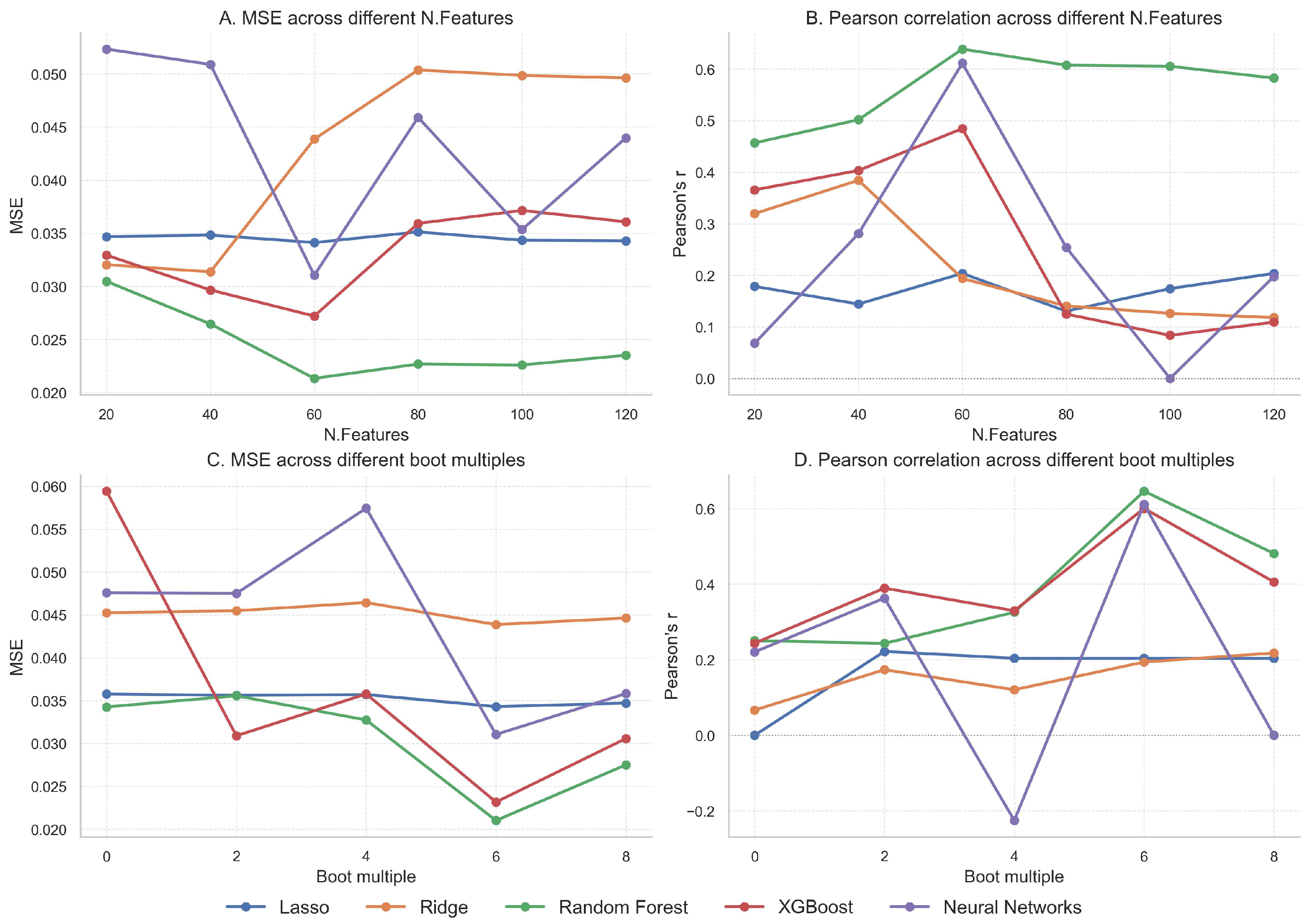
4.4.1. Effects of Feature Number and Bootstrap Augmentation
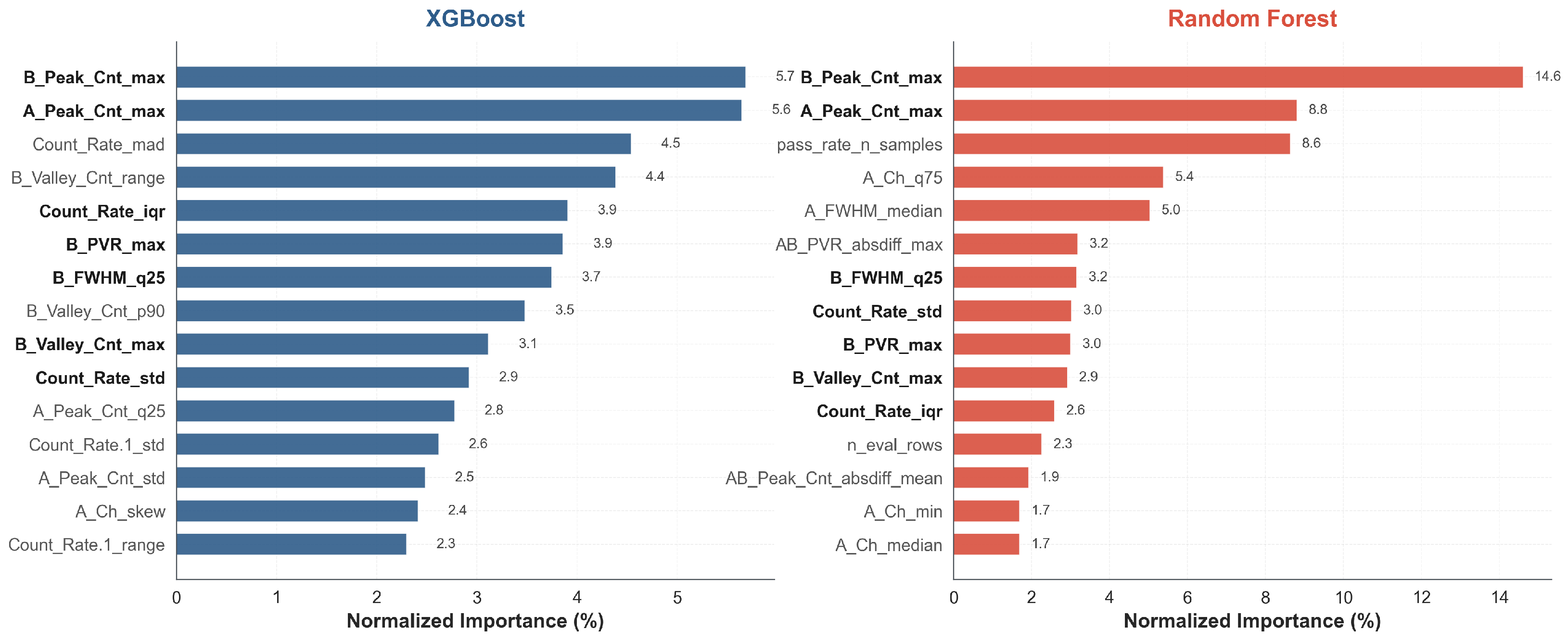
4.4.2. Feature Importance Analysis
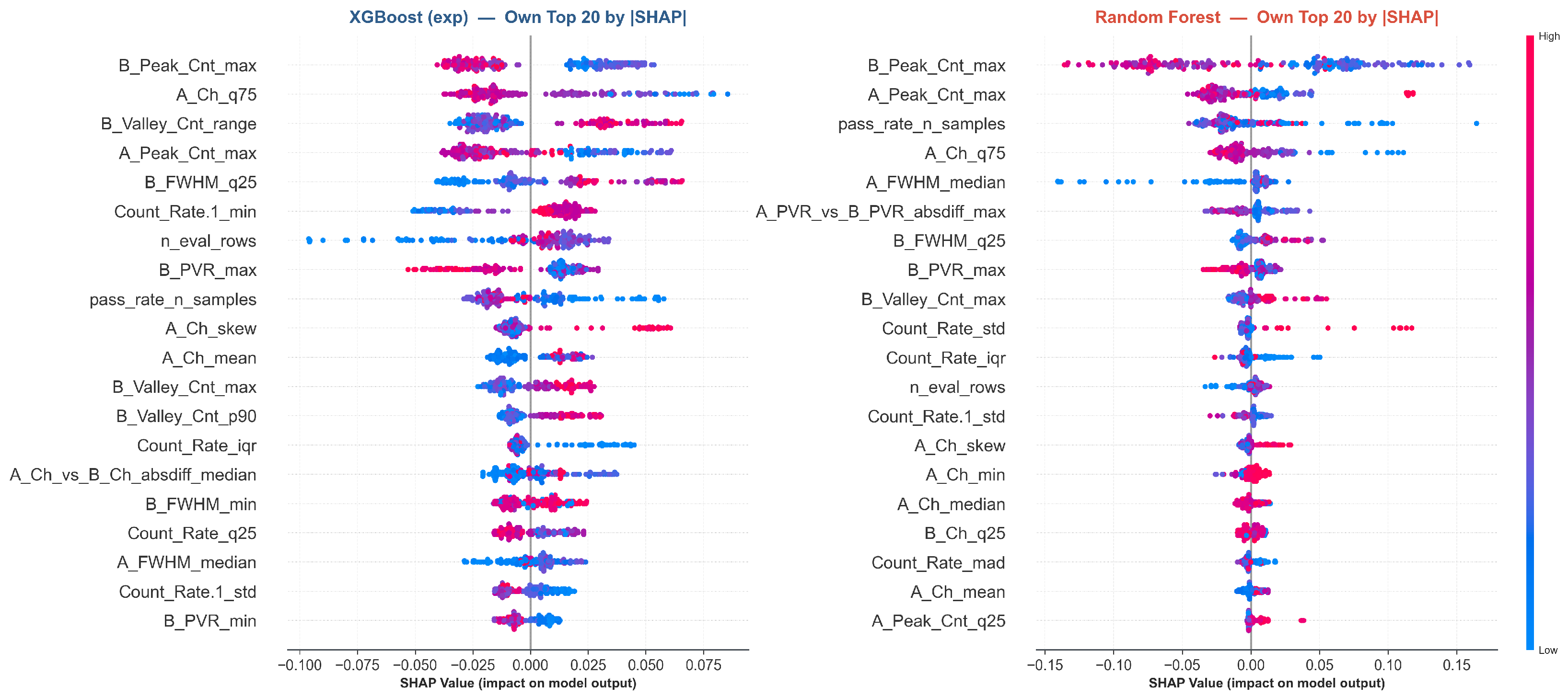
4.4.3. SHAP-Based Model Interpretation
4.5. Evaluation Experiment of Model Prediction and Empirical Rules
5. Discussion
6. Conclusions
Author Contributions
Funding
Institutional Review Board Statement
Informed Consent Statement
Data Availability Statement
Acknowledgments
Conflicts of Interest
Abbreviations
| CZT | Cadmium Zinc Telluride |
| IV | Current–Voltage |
| FWHM | Full Width at Half Maximum |
| RF | Random Forest |
| LR | Linear Regression |
| MLR | Multiple Linear Regression |
| FNN | Feedforward Neural Network |
| MAE | Mean Absolute Error |
| RMSE | Root Mean Squared Error |
| MSE | Mean Squared Error |
Appendix A. Raw Dataset Format

| Block | Example Raw Columns | Description |
|---|---|---|
| Product/test-wafer block | Code, Spec, IV_Voltage, IV_Neg, IV_Pos, IV_Graph, Result | Downstream product-wafer records. These fields describe the product/test-wafer specification, IV testing condition, IV current response, IV-curve morphology, and final pass/fail judgement. The pass/fail judgements in this block were aggregated at the ingot level to construct the regression target. |
| Evaluation-wafer identification and acquisition block | Eval_Code, Eval_Spec, Source, Eval_IV_Voltage, Eval_IV_Neg, Eval_IV_Pos, Eval_IV_Graph, Pref_Side | Evaluation-wafer identifiers, standardized evaluation-wafer specification, radiation source, IV acquisition parameters, IV responses, IV-curve morphology, and preferred measurement orientation. These fields provide standardized characterization information for each ingot. |
| Evaluation-wafer A-surface spectral block | A_Bias, A_Ch, A_FWHM, A_Res, A_Peak_Cnt, A_Valley_Cnt, A_PVR, A_Peak_Desc, Front_Ch(A), A_Noise_keV, A_Count_Rate | A-surface electrical and spectral measurements of evaluation wafers, including bias voltage, peak-channel position, FWHM, energy resolution, peak and valley counts, peak-to-valley ratio, peak description, front-channel value, noise level, and count rate when available. |
| Evaluation-wafer B-surface spectral block | B_Bias, B_Ch, B_FWHM, B_Res, B_Peak_Cnt, B_Valley_Cnt, B_PVR, B_Peak_Desc, Front_Ch(B), B_Noise_keV, B_Count_Rate | B-surface electrical and spectral measurements of evaluation wafers. Together with the A-surface block, these fields enable the quantification of double-sided response consistency and surface asymmetry. |
Appendix B. Feature Abbreviations and Raw-Feature Correlation Analysis
Appendix B.1. Feature Abbreviation Rules
| Feature Name or Suffix | Meaning and Interpretation |
|---|---|
| A_, B_ | Measurements from the A or B surface of the wafer. They represent double-sided detector responses and may reflect surface-dependent electrical or spectral behavior. |
| IV | Current–voltage or leakage-current-related descriptor. It reflects electrical leakage behavior under the specified bias condition. |
| FWHM | Full width at half maximum, describing spectral energy resolution. Smaller values generally indicate better resolution. |
| Peak_Cnt | Photopeak count, representing spectral signal strength. Its effect may depend on noise level, FWHM, and count-rate stability. |
| Valley_Cnt | Valley or background count, characterizing background contribution near the spectral valley and related noise behavior. |
| PVR | Peak-to-valley ratio, a signal-to-background descriptor derived from peak and valley counts. |
| Count_Rate | Count-rate measurement, reflecting detection rate and measurement stability. |
| Ch | Channel or peak-channel-related descriptor, associated with spectral peak position or calibration behavior. |
| _mean, _median | Mean or median across evaluation wafers within an ingot, describing the central tendency of an ingot-level measurement. |
| _std, _cv | Standard deviation or coefficient of variation, quantifying wafer-to-wafer variability within an ingot. |
| _min, _max, _range | Minimum, maximum, or range across evaluation wafers, capturing extreme values and overall dispersion. |
| _q10, _q25, _q75, _q90 | Percentile-based descriptors that characterize the within-ingot distribution and reduce sensitivity to isolated outliers. |
| _iqr | Interquartile range, measuring the spread between the 25th and 75th percentiles. |
| _mad | Median absolute deviation, a robust descriptor of within-ingot variability. |
| _skew, _kurtosis | Skewness and kurtosis, describing asymmetry and tail behavior of the within-ingot distribution. |
| _absdiff_ | Absolute difference between corresponding A- and B-side descriptors, quantifying surface-to-surface asymmetry. |
| pass_rate | Proportion of evaluation wafers satisfying a predefined threshold or empirical pass/fail rule. |
| n_eval_rows | Number of valid evaluation-wafer records for an ingot, indicating the amount of available evaluation information. |
| pass_rate_n_samples | Sample-size-related descriptor associated with pass-rate estimation. It helps account for different numbers of evaluation wafers. |
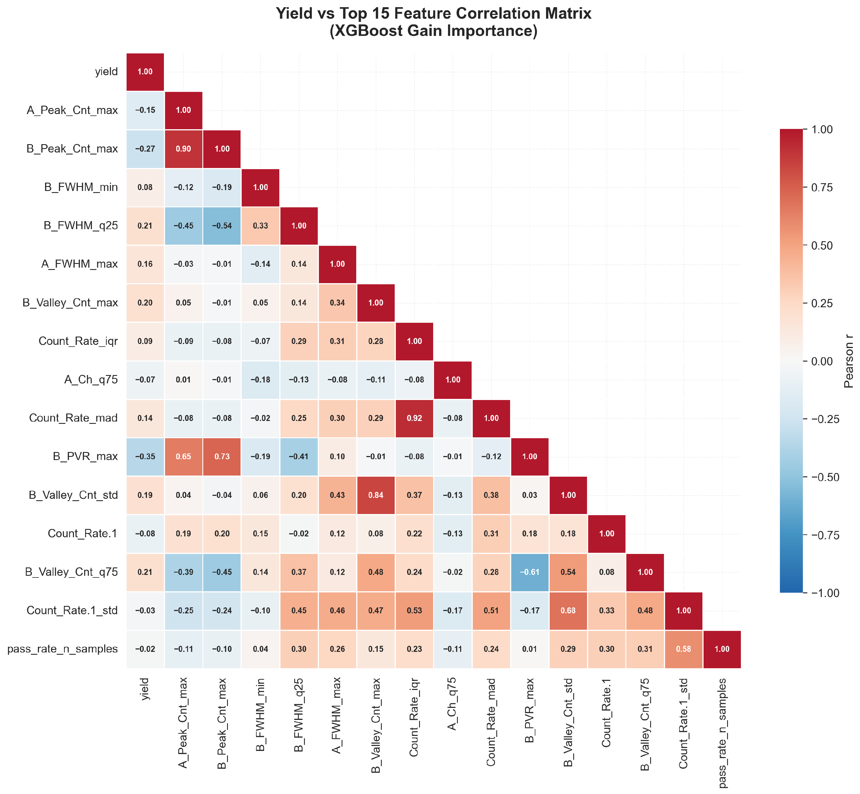
Appendix B.2. Correlation Analysis of Top-Ranked Engineered Features Selected by XGBoost Importance

Appendix C
| Model | MSE (CI) | MAE (CI) | Pearson’s r (CI) | Spearman’s (CI) |
|---|---|---|---|---|
| Boot = 0 | ||||
| Mean | 0.036 (0.016–0.060) | 0.144 (0.090–0.203) | 0.000 (0.000–0.000) | 0.000 (0.000–0.000) |
| MLR | 0.270 (0.128–0.473) | 0.414 (0.287–0.571) | 0.145 (−0.115–0.383) | 0.183 (−0.264–0.497) |
| Lasso | 0.036 (0.016–0.060) | 0.144 (0.090–0.203) | 0.000 (0.000–0.000) | 0.000 (0.000–0.000) |
| Ridge | 0.045 (0.019–0.075) | 0.166 (0.106–0.228) | 0.067 (−0.417–0.517) | 0.061 (−0.420–0.568) |
| RF | 0.034 (0.017–0.054) | 0.147 (0.094–0.200) | 0.251 (−0.188–0.591) | 0.282 (−0.230–0.651) |
| XGBoost | 0.059 (0.033–0.096) | 0.207 (0.151–0.271) | 0.244 (−0.134–0.571) | 0.316 (−0.108–0.647) |
| NN | 0.048 (0.022–0.074) | 0.178 (0.118–0.233) | 0.221 (−0.202–0.609) | 0.261 (−0.181–0.670) |
| Boot = 2 | ||||
| Mean | 0.036 (0.016–0.060) | 0.144 (0.090–0.203) | 0.000 (0.000–0.000) | 0.000 (0.000–0.000) |
| MLR | 0.057 (0.036–0.082) | 0.209 (0.158–0.261) | 0.284 (0.004–0.592) | 0.251 (−0.134–0.667) |
| Lasso | 0.036 (0.016–0.059) | 0.144 (0.090–0.202) | 0.222 (−0.356–0.690) | 0.247 (−0.422–0.751) |
| Ridge | 0.046 (0.025–0.069) | 0.183 (0.136–0.234) | 0.174 (−0.214–0.555) | 0.141 (−0.294–0.566) |
| RF | 0.036 (0.020–0.054) | 0.160 (0.113–0.207) | 0.243 (−0.201–0.592) | 0.131 (−0.402–0.552) |
| XGBoost | 0.031 (0.015–0.049) | 0.136 (0.086–0.189) | 0.390 (−0.032–0.696) | 0.323 (−0.183–0.730) |
| NN | 0.048 (0.027–0.069) | 0.185 (0.133–0.238) | 0.363 (−0.003–0.633) | 0.375 (−0.065–0.729) |
| Boot = 4 | ||||
| Mean | 0.036 (0.016–0.060) | 0.144 (0.090–0.203) | 0.000 (0.000–0.000) | 0.000 (0.000–0.000) |
| MLR | 0.046 (0.019–0.075) | 0.159 (0.105–0.220) | 0.295 (−0.026–0.601) | 0.401 (−0.087–0.742) |
| Lasso | 0.036 (0.016–0.059) | 0.144 (0.090–0.203) | 0.204 (−0.312–0.652) | 0.189 (−0.399–0.707) |
| Ridge | 0.046 (0.020–0.080) | 0.170 (0.116–0.234) | 0.121 (−0.368–0.535) | 0.183 (−0.349–0.626) |
| RF | 0.033 (0.017–0.052) | 0.147 (0.099–0.194) | 0.326 (0.026–0.654) | 0.356 (−0.057–0.784) |
| XGBoost | 0.036 (0.019–0.053) | 0.155 (0.107–0.202) | 0.330 (0.056–0.618) | 0.328 (−0.029–0.670) |
| NN | 0.057 (0.021–0.101) | 0.173 (0.105–0.249) | -0.226 (−0.700–0.299) | -0.129 (−0.662–0.504) |
| Boot = 6 | ||||
| Mean | 0.036 (0.016–0.059) | 0.144 (0.090–0.203) | 0.000 (0.000–0.000) | 0.000 (0.000–0.000) |
| MLR | 0.041 (0.018–0.071) | 0.155 (0.092–0.219) | 0.296 (−0.160–0.616) | 0.335 (−0.131–0.700) |
| Lasso | 0.034 (0.016–0.055) | 0.142 (0.089–0.197) | 0.204 (−0.312–0.652) | 0.189 (−0.399–0.707) |
| Ridge | 0.044 (0.021–0.073) | 0.164 (0.106–0.231) | 0.194 (−0.278–0.583) | 0.152 (−0.374–0.563) |
| RF | 0.021 (0.011–0.032) | 0.125 (0.090–0.163) | 0.646 (0.346–0.839) | 0.595 (0.262–0.817) |
| XGBoost | 0.023 (0.012–0.039) | 0.128 (0.089–0.168) | 0.601 (0.227–0.845) | 0.490 (0.011–0.796) |
| NN | 0.031 (0.018–0.047) | 0.149 (0.111–0.187) | 0.611 (0.272–0.824) | 0.643 (0.209–0.892) |
| Boot = 8 | ||||
| Mean | 0.036 (0.016–0.060) | 0.144 (0.090–0.203) | 0.000 (0.000–0.000) | 0.000 (0.000–0.000) |
| MLR | 0.046 (0.024–0.073) | 0.176 (0.127–0.234) | 0.201 (−0.240–0.587) | 0.183 (−0.276–0.643) |
| Lasso | 0.035 (0.016–0.057) | 0.143 (0.090–0.200) | 0.204 (−0.312–0.652) | 0.189 (−0.399–0.707) |
| Ridge | 0.045 (0.022–0.077) | 0.179 (0.131–0.233) | 0.218 (−0.296–0.652) | 0.222 (−0.327–0.687) |
| RF | 0.028 (0.014–0.044) | 0.139 (0.094–0.186) | 0.481 (0.024–0.754) | 0.352 (−0.140–0.750) |
| XGBoost | 0.031 (0.015–0.048) | 0.141 (0.095–0.193) | 0.406 (0.070–0.712) | 0.304 (−0.225–0.739) |
| NN | 0.036 (0.016–0.060) | 0.144 (0.090–0.203) | 0.000 (0.000–0.000) | 0.000 (0.000–0.000) |
References
- Fu, X.; Wang, F.B.; Zuo, X.R.; Wang, Z.J.; Wang, Q.R.; Wang, K.Q.; Xu, L.Y.; Xu, Y.D.; Guo, R.R.; Yu, H.; et al. Distinctive distribution of defects in CdZnTe: In ingots and their effects on the photoelectric properties. Chin. Phys. B 2018, 27, 037302. [Google Scholar] [CrossRef] [Scilit]
- Roy, U.N.; Camarda, G.; Cui, Y.; Gul, R.; Hossain, A.; Yang, G.; Zazvorka, J.; Dedic, V.; Franc, J.; James, R. Role of selenium addition to CdZnTe matrix for room-temperature radiation detector applications. Sci. Rep. 2019, 9, 1620. [Google Scholar] [CrossRef] [Scilit] [PubMed]
- Ballester, M.; Kaspar, J.; Massanés, F.; Banerjee, S.; Vija, A.H.; Katsaggelos, A.K. Characterization of Crystal Properties and Defects in CdZnTe Radiation Detectors. Crystals 2024, 14, 935. [Google Scholar] [CrossRef] [Scilit]
- Roy, U.N.; Camarda, G.S.; Cui, Y.; James, R.B. Optimization of selenium in CdZnTeSe quaternary compound for radiation detector applications. Appl. Phys. Lett. 2021, 118. [Google Scholar] [CrossRef] [Scilit]
- Kirschenmann, S.; Bezak, M.; Bharthuar, S.; Brücken, E.; Golovleva, M.; Gädda, A.; Kalliokoski, M.; Karadzhinova-Ferrer, A.; Koponen, P.; Kramarenko, N.; et al. Quality assessment of cadmium telluride as a detector material for multispectral medical imaging. J. Instrum. 2022, 17, C01070. [Google Scholar] [CrossRef] [Scilit]
- Amato, U.; Antoniadis, A.; De Feis, I.; Doinychko, A.; Gijbels, I.; La Magna, A.; Pagano, D.; Piccinini, F.; Selvan Suviseshamuthu, E.; Severgnini, C.; et al. Detecting Important Features and Predicting Yield from Defects Detected by SEM in Semiconductor Production. Sensors 2025, 25, 4218. [Google Scholar] [CrossRef] [Scilit] [PubMed]
- Chawla, N.V.; Bowyer, K.W.; Hall, L.O.; Kegelmeyer, W.P. SMOTE: Synthetic minority over-sampling technique. J. Artif. Intell. Res. 2002, 16, 321–357. [Google Scholar] [CrossRef] [Scilit]
- Kim, H.; Kim, J.; Cho, S. Application of SMOTE for semiconductor manufacturing process with class imbalance. In Proceedings of the Korean Operations Research and Management Science Conference; Korean Operations Research and Management Science Society: Seoul, Republic of Korea, 2017; pp. 345–365. [Google Scholar]
- Bai, J.; Wu, D.; Shelley, T.; Schubel, P.; Twine, D.; Russell, J.; Zeng, X.; Zhang, J. A Comprehensive Survey on Machine Learning Driven Material Defect Detection. ACM Comput. Surv. 2025, 57, 1–36. [Google Scholar] [CrossRef] [Scilit]
- Khan, K.; Walker, D.M.H. A review of yield modelling techniques for semiconductor manufacturing. Int. J. Prod. Res. 2024, 62, 6543–6562. [Google Scholar] [CrossRef] [Scilit]
- Wang, S.; Chen, Y. Improved Yield Prediction and Failure Analysis in Semiconductor Manufacturing with XGBoost and Shapley Additive exPlanations Models. In 2024 IEEE International Symposium on the Physical and Failure Analysis of Integrated Circuits (IPFA); IEEE: Piscataway, NJ, USA, 2024; p. 262. [Google Scholar] [CrossRef] [Scilit]
- Goldstein, H. Multilevel Statistical Models, 4th ed.; Wiley: Chichester, UK, 2011. [Google Scholar]
- Steele, F. Multilevel models for longitudinal data. J. R. Stat. Soc. Ser. A (Stat. Soc.) 2008, 171, 5–19. [Google Scholar] [CrossRef] [Scilit]
- Groß, J. Linear Regression; Springer Science & Business Media: Berlin/Heidelberg, Germany, 2003; Volume 175. [Google Scholar]
- Marquardt, D.W.; Snee, R.D. Ridge regression in practice. Am. Stat. 1975, 29, 3–20. [Google Scholar] [CrossRef] [Scilit]
- Ranstam, J.; Cook, J.A. LASSO regression. J. Br. Surg. 2018, 105, 1348. [Google Scholar] [CrossRef] [Scilit]
- Breiman, L. Random forests. Mach. Learn. 2001, 45, 5–32. [Google Scholar] [CrossRef] [Scilit]
- Chen, T.; Guestrin, C. XGBoost: A Scalable Tree Boosting System. In Proceedings of the 22nd ACM SIGKDD International Conference on Knowledge Discovery and Data Mining; Association for Computing Machinery: New York, NY, USA, 2016. [Google Scholar]
- LeCun, Y.; Touresky, D.; Hinton, G.; Sejnowski, T. A theoretical framework for back-propagation. In Proceedings of the 1988 Connectionist Models Summer School; Carnegie Mellon University: Pittsburgh, PA, USA, 1988; Volume 1, pp. 21–28. [Google Scholar]
- Bebis, G.; Georgiopoulos, M. Feed-forward neural networks. IEEE Potentials 2002, 13, 27–31. [Google Scholar] [CrossRef] [Scilit]
- Krogh, A.; Hertz, J. A simple weight decay can improve generalization. In Proceedings of the 5th International Conference on Neural Information Processing Systems; Morgan Kaufmann Publishers Inc.: San Francisco, CA, USA, 1991. [Google Scholar]
- Srivastava, N.; Hinton, G.; Krizhevsky, A.; Sutskever, I.; Salakhutdinov, R. Dropout: A simple way to prevent neural networks from overfitting. J. Mach. Learn. Res. 2014, 15, 1929–1958. [Google Scholar]
- Efron, B. Bootstrap methods: Another look at the jackknife. Ann. Stat. 1979, 7, 1–26. [Google Scholar] [CrossRef] [Scilit]
- Hesterberg, T. Bootstrap. Wiley Interdiscip. Rev. Comput. Stat. 2011, 3, 497–526. [Google Scholar] [CrossRef] [Scilit]
- Bergstra, J.; Bengio, Y. Random search for hyper-parameter optimization. J. Mach. Learn. Res. 2012, 13, 281–305. [Google Scholar]
- Snoek, J.; Larochelle, H.; Adams, R.P. Practical bayesian optimization of machine learning algorithms. In Proceedings of the 26th International Conference on Neural Information Processing Systems; Curran Associates Inc.: Red Hook, NY, USA, 2012. [Google Scholar]
- Browne, M.W. Cross-validation methods. J. Math. Psychol. 2000, 44, 108–132. [Google Scholar] [CrossRef] [Scilit] [PubMed]
- Pedregosa, F.; Varoquaux, G.; Gramfort, A.; Michel, V.; Thirion, B.; Grisel, O.; Blondel, M.; Prettenhofer, P.; Weiss, R.; Dubourg, V.; et al. Scikit-learn: Machine learning in Python. J. Mach. Learn. Res. 2011, 12, 2825–2830. [Google Scholar]


| Setting | Model | MSE (95% CI) | MAE (95% CI) | Pearson’s r (95% CI) |
|---|---|---|---|---|
| Baseline (Boot = 0) | Mean | 0.036 (0.016–0.060) | 0.144 (0.090–0.203) | NA |
| MLR | 0.270 (0.128–0.473) | 0.414 (0.287–0.571) | 0.145 (−0.115–0.383) | |
| Lasso | 0.036 (0.016–0.060) | 0.144 (0.090–0.203) | NA | |
| Ridge | 0.045 (0.019–0.075) | 0.166 (0.106–0.228) | 0.067 (−0.417–0.517) | |
| RF | 0.034 (0.017–0.054) | 0.147 (0.094–0.200) | 0.251 (−0.188–0.591) | |
| XGBoost | 0.059 (0.033–0.096) | 0.207 (0.151–0.271) | 0.244 (−0.134–0.571) | |
| NN | 0.048 (0.022–0.074) | 0.178 (0.118–0.233) | 0.221 (−0.202–0.609) | |
| Augmentation (Boot = 6) | Mean | 0.036 (0.016–0.059) | 0.144 (0.090–0.203) | NA |
| MLR | 0.041 (0.018–0.071) | 0.155 (0.092–0.219) | 0.296 (−0.160–0.616) | |
| Lasso | 0.034 (0.016–0.055) | 0.142 (0.089–0.197) | 0.204 (−0.312–0.652) | |
| Ridge | 0.044 (0.021–0.073) | 0.164 (0.106–0.231) | 0.194 (−0.278–0.583) | |
| RF | 0.021 (0.011–0.032) | 0.125 (0.090–0.163) | 0.646 (0.346–0.839) | |
| XGBoost | 0.023 (0.012–0.039) | 0.128 (0.089–0.168) | 0.601 (0.227–0.845) | |
| NN | 0.031 (0.018–0.047) | 0.149 (0.111–0.187) | 0.611 (0.272–0.824) |
| Method | Top22% Avg | Rest Avg | Improvement | p-Value |
|---|---|---|---|---|
| XGBoost | 60.40 | 33.87 | 26.53 | 0.0083 |
| RF | 63.71 | 32.92 | 30.79 | 0.0026 |
| Rule_IV_Abs | 59.08 | 34.23 | 24.85 | 0.0307 |
| Rule_IV_Shape | 43.15 | 38.80 | 4.36 | 0.3352 |
| XGBoost + Abs | 61.94 | 33.43 | 28.51 | 0.0052 |
| RF + Abs | 63.71 | 32.92 | 30.79 | 0.0026 |
Disclaimer/Publisher’s Note: The statements, opinions and data contained in all publications are solely those of the individual author(s) and contributor(s) and not of MDPI and/or the editor(s). MDPI and/or the editor(s) disclaim responsibility for any injury to people or property resulting from any ideas, methods, instructions or products referred to in the content. |
© 2026 by the authors. Licensee MDPI, Basel, Switzerland. This article is an open access article distributed under the terms and conditions of the Creative Commons Attribution (CC BY) license.
Share and Cite
Jie, R.; Yang, F.; Xi, S.; Tang, S.; Jie, W. Yield Prediction Model for Ingot Samples Based on Machine Learning and Data Augmentation. Crystals 2026, 16, 387. https://doi.org/10.3390/cryst16060387
Jie R, Yang F, Xi S, Tang S, Jie W. Yield Prediction Model for Ingot Samples Based on Machine Learning and Data Augmentation. Crystals. 2026; 16(6):387. https://doi.org/10.3390/cryst16060387
Chicago/Turabian StyleJie, Renlong, Fan Yang, Shouzhi Xi, Sanqi Tang, and Wanqi Jie. 2026. "Yield Prediction Model for Ingot Samples Based on Machine Learning and Data Augmentation" Crystals 16, no. 6: 387. https://doi.org/10.3390/cryst16060387
APA StyleJie, R., Yang, F., Xi, S., Tang, S., & Jie, W. (2026). Yield Prediction Model for Ingot Samples Based on Machine Learning and Data Augmentation. Crystals, 16(6), 387. https://doi.org/10.3390/cryst16060387