Development and Experimental Validation of a Thin-Film Thermocouple System for Real-Time Temperature Monitoring and Tool Wear Prediction in Cutting Processes

Abstract

A homemade NiCr/NiSi thin-film thermocouple integrated with a PCBN turning tool was developed for real-time temperature monitoring during dry turning of AISI 1045 steel. The study addresses a practical limitation of existing cutting-temperature methods, namely the difficulty of combining local in situ sensing near the cutting edge with a transient thermal analysis framework that can interpret the measured signal under repeatable cutting conditions. The sensor was fabricated on an Al₂O₃ substrate by magnetron sputtering, protected by a SiO₂ layer, and tested at cutting speeds corresponding to spindle speeds of 1000, 1500 and 2000 rpm, with a cutting depth of 0.5 mm, a feed rate of 0.1 mm/rev and cutting times of 30–90 s. A three-dimensional transient heat-conduction model and inverse heat-flux reconstruction were then used to interpret the temperature history. The maximum measured temperature increased from 342 °C to 488 °C, and VB increased from 0.082 mm to 0.295 mm, showing a strong temperature–wear association within the investigated parameter window.

1. Introduction

Cutting temperature is one of the key state variables in machining because it affects heat partition, tool wear, dimensional accuracy and surface integrity. Reliable temperature measurement close to the cutting edge is therefore essential for understanding thermo-mechanical loading and for developing online tool-condition monitoring methods. Thin-film thermocouples are attractive in this context because of their small thermal mass, fast response and ability to be integrated near the tool–chip contact zone.

Previous studies have demonstrated the feasibility of built-in or surface-deposited thin-film thermocouples for monitoring cutting temperature, and related inverse heat-conduction methods have been used to reconstruct interfacial thermal loads from measured temperature histories. However, the literature also shows two persistent limitations: first, many studies focus mainly on sensor fabrication or calibration without linking the measured signal to a physically interpretable thermal boundary condition; second, differences in sensor layout, substrate material, deposition route and cutting configuration make the reported results difficult to compare directly and limit their use for synchronous temperature–wear evaluation in turning.

Accordingly, the specific research question of this work is whether a homemade NiCr/NiSi thin-film thermocouple integrated close to the cutting edge can provide stable in situ temperature data during dry turning, and whether these data can be coupled with inverse thermal analysis to interpret the association among cutting conditions, tool temperature, interface heat flux and flank wear. Compared with broader reviews on thin-film thermocouples and Seebeck-based temperature sensing, the present study focuses specifically on the combined sensor-design-plus-application problem in turning [1,2,3].

To address this gap, the present work develops a homemade NiCr/NiSi thin-film thermocouple on an Al₂O₃ substrate with a SiO₂ protective layer and integrates it with a PCBN cutting tool for dry turning of AISI 1045 steel. The main contribution is not only the fabrication of the sensing element itself, but also the establishment of a sensor-experiment-inverse-analysis framework that enables repeatable cutting tests, signal interpretation and temperature–wear correlation analysis under clearly reported conditions.

Recent work most closely related to the present topic includes tool-integrated thin-film thermocouples for cutting temperature measurement, inverse estimation of tool–chip interface temperature fields, and thin-film thermocouple performance studies in machining environments [4,5,6,7,8]. In contrast, more general background on thin-film thermocouples is citedonly where needed to explain the sensing principle and material selection.

The remainder of the paper first explains the sensing principle and the structure of the developed sensor, then presents the fabrication and experimental methodology, followed by the inverse numerical procedure, the temperature and wear results, and the corresponding discussion of measurement reliability and thermo-mechanical interpretation.

2. Principle of Thin-Film Thermocouples

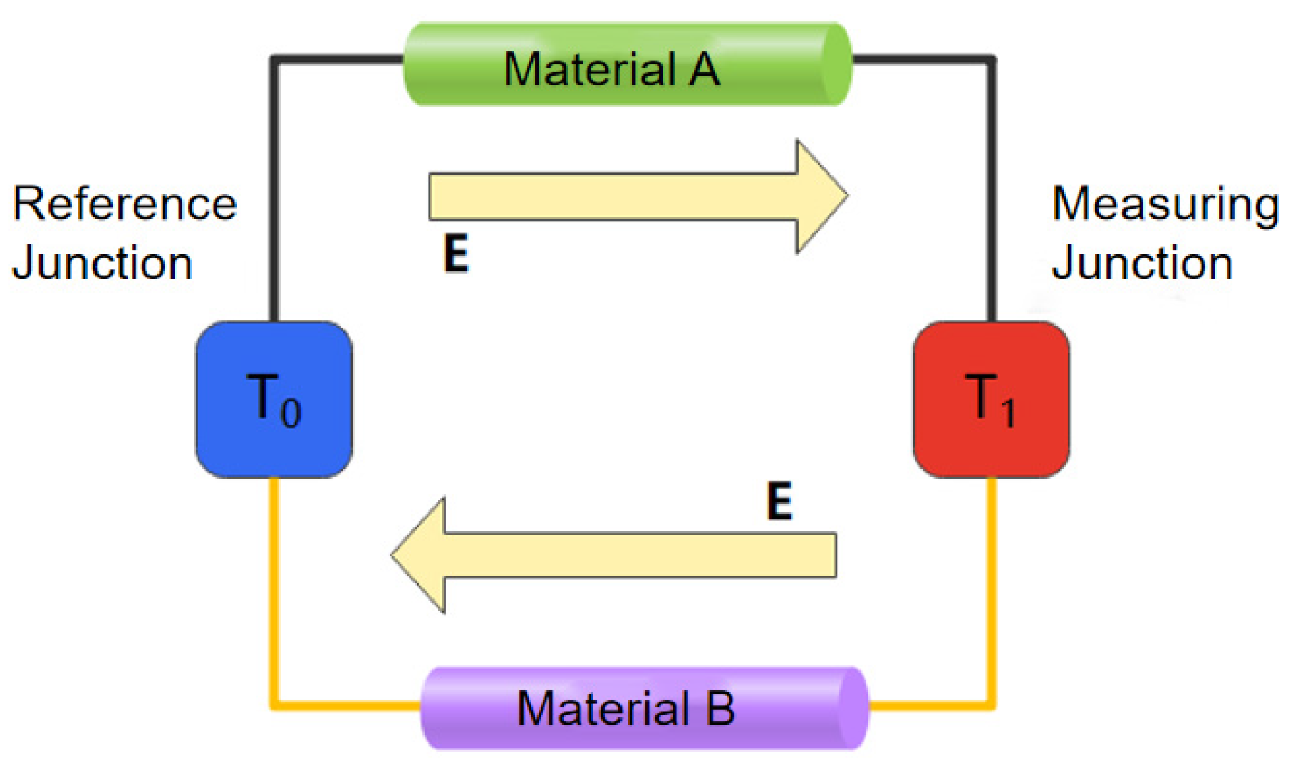
The temperature measurement principle of the developed thin-film thermocouple is based on the Seebeck effect. When two dissimilar conductive materials form a closed circuit, and the two junctions are at different temperatures, a thermoelectric potential is generated. In the present sensor, the NiCr and NiSi thin-film electrodes form the measurement loop, the hot junction is located on the rake face close to the cutting edge, and the cold junction is routed to a relatively thermally stable position inside the holder and maintained at 25 °C during calibration and testing. Standard treatments of this principle for thin-film sensors can be found in Taylor and Pollock [9] and in the review by Zhang and Wang [10].

During cutting, the hot junction senses the local transient thermal load generated near the tool–chip interface, while the cold junction provides the reference temperature. The measured thermoelectric voltage is acquired by the data-acquisition system and converted to temperature using the static calibration curve of the fabricated sensor. In this way, the sensor output is not treated as an abstract voltage signal; rather, it is used to estimate the hot-junction temperature close to the cutting zone and then serves as the experimental input for the inverse heat-conduction analysis.

$$S_{\mathrm{AB}}={ V}_1 -{ V}_2/T_{1 }-{ T}_0$$

(1)

In Equation (1), S_AB denotes the Seebeck coefficient of the NiCr/NiSi thermocouple pair, (V₁ − V₂) is the measured thermoelectric potential difference, T₁ is the hot-junction temperature, and T₀ is the cold-junction temperature. Rearrangement of the calibrated voltage–temperature relation allows T₁ to be determined when T₀ is known and the thermoelectric potential is measured. In the present work, the practical temperature calculation was based on the sensor calibration curve, while Equation (1) was used to express the governing thermoelectric relationship and to check consistency between voltage output and measured temperature difference. A schematic diagram illustrating the temperature measurement principle of a thin-film thermocouple is shown in Figure 1.

3. Design of Thin-Film Thermocouple Samples

3.1. Sensor Structure and Fabrication Process

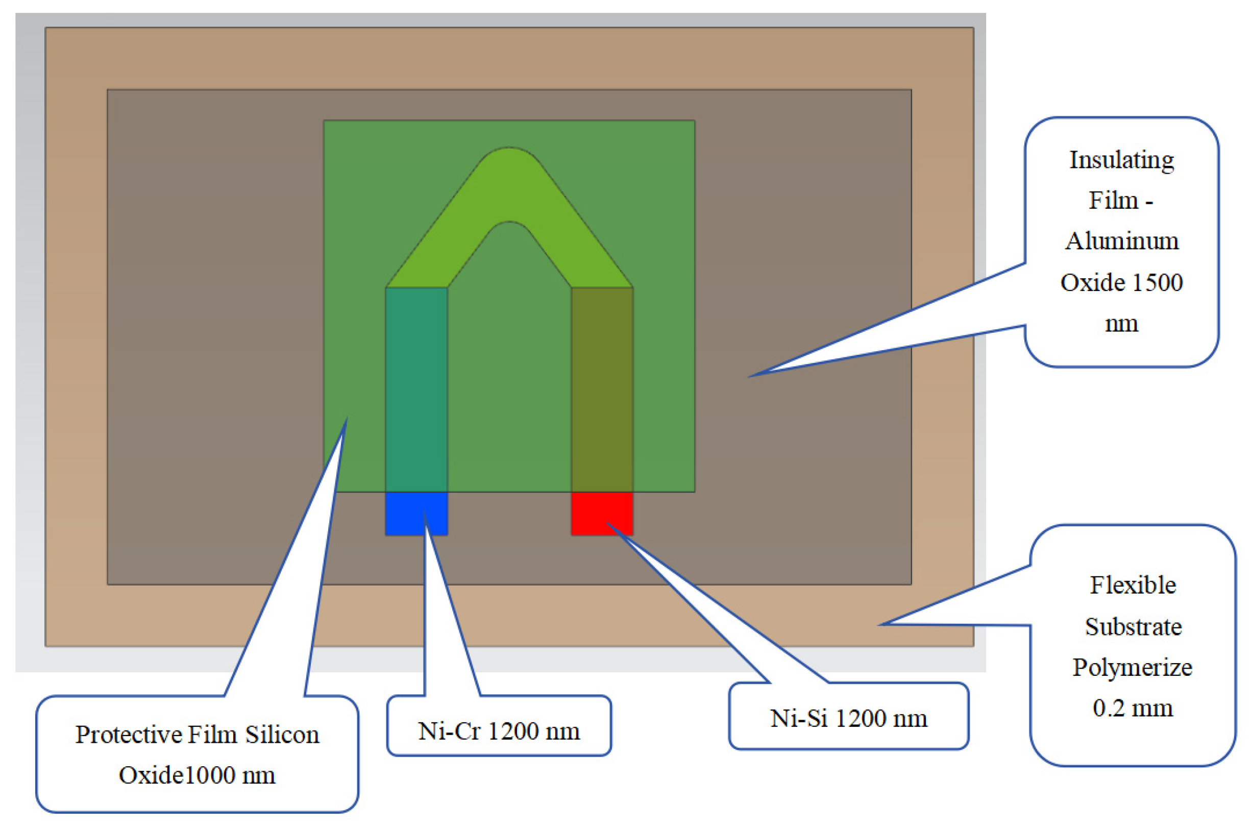
Figure 2 shows the geometry of the thin-film thermocouple sample. In this work, the sensor was homemade by depositing the functional layers on an Al₂O₃ substrate using magnetron sputtering and then integrating the fabricated sensing element with the cutting tool. The fabrication route included substrate cleaning, deposition of the insulating layer, deposition and patterning of the NiCr/NiSi thermoelectric electrodes, and deposition of the SiO₂ protective layer. Because reproducibility of the sensor strongly depends on the preparation route, the key equipment and process parameters are reported here as part of the experimental methodology rather than as a purely descriptive design note.

Magnetron sputtering was selected because it provides dense and uniform films, stable composition control and good interfacial adhesion, all of which are important for thermoelectric stability and long-term durability of thin-film sensors in cutting environments [11,12]. In the present study, the fabrication parameters are reported mainly to clarify how the designed sensing structure was actually realised and to enable reproduction of the deposited layer system.

A thin-film thermocouple’s substrate material must provide stable mechanical support for the thermoelement film, while also exhibiting excellent high-temperature resistance and reliable electrical insulation. It must also have a low thermal expansion coefficient. These properties are essential in order to prevent cracking or delamination of the thin film caused by thermal stress during temperature fluctuations, thereby ensuring measurement accuracy and extending the sensor’s service life [11,13]. Among the available substrate materials, alumina (Al₂O₃) ceramic is an ideal candidate. With a high melting point of 2054 °C, Al₂O₃ maintains its structural integrity at high temperatures without softening, deforming, or degrading [14,15,16,17]. Furthermore, its high volume resistivity (10¹⁴–10¹⁶ Ω·cm at room temperature) effectively suppresses electrical leakage between the substrate and thermoelement layers, ensuring stable signal output [18,19,20].

In addition, the thermal expansion coefficient of Al₂O₃ (7.5 × 10⁻⁶/°C) is reasonably compatible with that of commonly used thermocouple materials, such as Ni-Cr (13 × 10⁻⁶/°C) and Ni-Si (11 × 10⁻⁶/°C) [21,22,23]. A comparison of the properties of commonly used ceramic materials is shown in

Table 1. Comparison of properties of common ceramic materials (dry turning, cutting depth 0.5 mm, feed rate 0.1 mm/rev).

Material	Maximum Service Temperature (°C)	Properties
Quartz (SiO2)	1100	Good heat resistance and impact resistance; low strength, susceptible to acid–base corrosion
Alumina (Al2O3, 99%)	1800	High strength, wear resistance, corrosion resistance, and good insulation
Magnesium oxide (MgO, 97%)	-	Hydrolysis-prone, corrosion-resistant
Zirconia	2400	Strong oxidation resistance; susceptible to alkaline corrosion

.

This thermal compatibility helps minimise interfacial stress during rapid heating and cooling, thereby reducing the likelihood of film delamination or structural failure. Taking these factors into account, a high-purity Al₂O₃ ceramic with a thickness of 1500 nm and a purity of 99.999% was selected as the substrate material, meeting the stringent mechanical and thermal requirements of high-speed turning environments [17]. In this study, the specific details of the magnetron sputtering equipment used to prepare NiCr/NiSi thermoelectric electrodes, Al₂O₃ insulating layers, and SiO₂ protective layers are as follows:

Equipment Model: JGP-450C Multi-Target Magnetron Sputtering Coating Machine (Manufactured in Shenyang, China, by Shenyang Baili High Vacuum Technology Co., Ltd.).

Core Configuration: Four independent sputtering target positions (target dimensions: Ф60 mm × 3 mm), supporting both DC Magnetron Sputtering and RF Magnetron Sputtering modes. Vacuum System: Utilises a combination of molecular pumps and mechanical pumps, achieving an ultimate vacuum of 5 × 10⁻⁵ Pa. Additionally equipped with a programmable temperature controller (range: 25–300 °C) and plasma diagnostic system (Langmuir probe).

Process Adaptability: Supports continuous multi-target sputtering for integrated deposition of insulating, functional, and protective layers without sample transfer, eliminating atmospheric exposure effects on film adhesion. The high vacuum environment (≤5 × 10⁻⁵ Pa) effectively minimises oxygen impurities in the film, ensuring the electrical conductivity and thermal stability of NiCr/NiSi thermoelectric electrodes. Al₂O₃ Insulating Layer (1500 nm): Deposited using RF magnetron sputtering with 99.999% high-purity Al₂O₃ ceramic as the target. Sputtering power: 120 W. Sputtering pressure: 0.6 Pa. Argon flow rate: 30 sccm. Substrate temperature: 200 °C. Deposition rate: 0.5 nm/s.

NiCr/NiSi thermoelectric electrodes (1200 nm each): Employed DC magnetron sputtering mode with Ni80Cr20 alloy target (99.99%) and Ni97Si3 alloy target (99.99%), respectively. Sputtering power: 80 W. Sputtering pressure: 0.4 Pa. Argon flow rate: 25 cm³/min. Substrate temperature: 150 °C. Deposition rate: 0.8 nm/s. Precise alignment of both electrodes and formation of the thermal bond were achieved using the equipment’s mask positioning function.

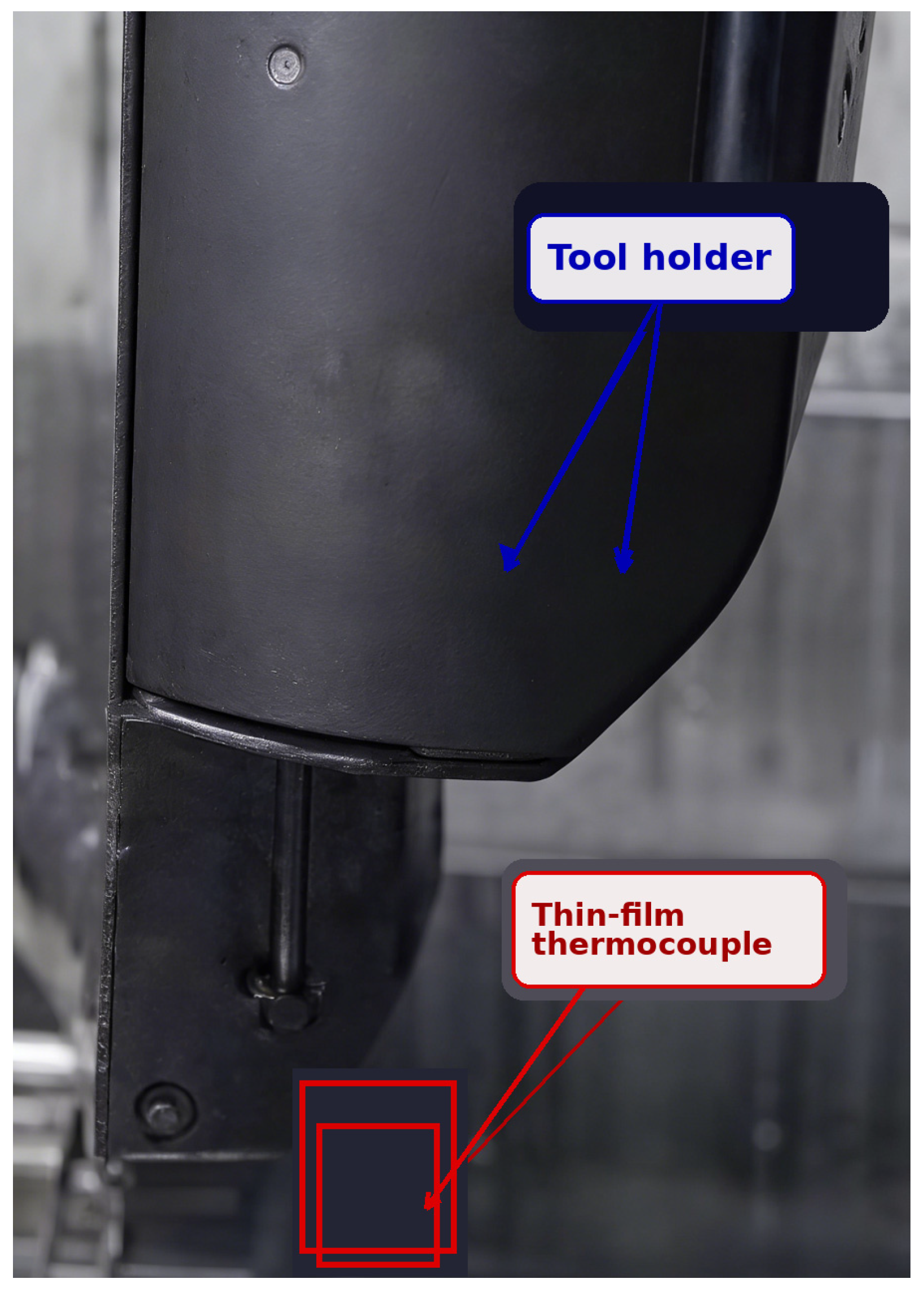
SiO₂ protective layer (1000 nm): Employed RF magnetron sputtering mode using 99.999% high-purity SiO₂ ceramic as the target material. Sputtering power: 100 W. Sputtering pressure: 0.5 Pa. Argon flow rate: 28 cm³/min. Substrate temperature: 180 °C. Deposition rate: 0.4 nm/s. The cutting tool schematic is shown in Figure 3.

3.2. Selection of Thin-Film Thermocouple Electrodes and Substrate Materials

The two dissimilar conductors that form the sensing junction of the thin-film thermocouple are made of thermoelectrode materials. According to the principles of thermoelectric conversion, any two distinct conductive materials can be combined to form a thermocouple if they are arranged in a closed circuit. In the present design, the thin-film thermocouple temperature sensor is intended for use in a turning environment where high thermal loads, rapid temperature fluctuations and mechanical stresses require robust thermoelectric and thermal properties in the materials used.

Among the thermoelement combinations used for thin-film thermocouples, NiCr/NiSi was selected because it offers a practical balance of Seebeck sensitivity, thermal stability, oxidation resistance, electrical conductivity and process compatibility with magnetron sputtering. Compared with some alternative metallic pairs, this combination is well established for medium-to-high temperature sensing and remains relatively cost-effective for tool-integrated fabrication. For the present application, these characteristics were considered more important than maximising the Seebeck coefficient alone, because stable signal output and film integrity during repeated cutting thermal cycles were critical design targets.

The substrate, serving as the core support structure for the thin-film thermocouple, must provide mechanical support, high-temperature resistance, electrical insulation and thermal-expansion compatibility. Al₂O₃ was selected not only because of its high-temperature resistance capability and insulation performance, but also because it offers a more balanced combination of thermal compatibility, surface stability and deposition suitability than quartz, MgO or zirconia for the present NiCr/NiSi film system. Thus, the contribution of the sensor design lies in the deliberate selection of a compatible electrode–substrate–protective-layer combination rather than in the use of any single material alone.

Excellent high-temperature stability: Al₂O₃ possesses a melting point of 2054 °C, significantly exceeding the measured temperature range of 342–488 °C during cutting operations. It exhibits no softening, deformation, or degradation at elevated temperatures, providing stable mechanical support for the NiCr/NiSi thermoelectric electrode film and SiO₂ protective layer while withstanding transient thermal shocks during dry cutting.

Reliable electrical insulation: At room temperature, Al₂O₃ exhibits a volume resistivity of 10¹⁴–10¹⁶ Ω·cm, effectively preventing electrical leakage between thermoelectric electrodes and tool substrates. This ensures a stable thermoelectric signal output and avoids measurement errors caused by insulation failure.

Excellent thermal expansion matching: Al₂O₃’s thermal expansion coefficient of 7.5 × 10⁻⁶/°C closely aligns with NiCr (13 × 10⁻⁶/°C) and NiSi (11 × 10⁻⁶/°C) thermoelectric materials. This minimises thermal stress at interfaces caused by rapid temperature fluctuations during cutting, reducing the risk of film delamination.

Compatibility with Magnetron Sputtering Process: High-purity Al₂O₃ exhibits excellent surface flatness and dense structure, achieving strong adhesion with magnetron-sputtered films (measured adhesion > 15 N). This ensures structural integrity after 1000 thermal shock cycles, meeting durability requirements for industrial batch processing.

Compared to other ceramic materials like quartz (SiO₂, high-temperature resistance up to 1100 °C but poor acid/alkali corrosion resistance), magnesium oxide (MgO, prone to hydrolysis), and zirconia (vulnerable to alkaline corrosion), Al₂O₃ offers superior comprehensive performance in high-temperature resistance, electrical insulation, thermal compatibility, and mechanical strength. This makes it the ideal substrate material for thin-film thermocouples used in cutting temperature measurement.

3.3. Selection of Protective Film Materials

Exposure of thermoelement films to ambient air over a long period of time can lead to oxidation through reactions with water vapour and oxygen. This results in increased electrical resistance, degraded signal accuracy and, in severe cases, delamination or peeling of the thin film [24,25]. To mitigate these effects, a protective layer is deposited after fabrication of the functional thermoelement films, providing electrical insulation and environmental protection [26,27,28].

Among the most commonly used protective materials, silicon dioxide (SiO₂) is particularly well-suited to thin-film thermocouples thanks to its dense microstructure, excellent oxidation resistance, strong corrosion and wear resistance, and stable performance at elevated temperatures [29,30]. These properties enable SiO₂ to effectively shield Ni-Cr/Ni-Si thermoelement films from oxidative degradation and mechanical damage, particularly from chip–tool interactions on the rake face during machining. Based on these advantages, a 1000 nm-thick SiO₂ film was selected as the protective layer in this study to ensure the long-term stability and reliability of the sensor under cutting conditions [31,32,33,34].

3.4. IHCP Solution and Heat Flow Inversion Workflow

A numerical procedure was used to reconstruct the transient heat flux at the tool–chip interface from the measured tool temperature. A three-dimensional transient thermal model of the PCBN insert and tool holder was established in ANSYS APDL. The insert, substrate and neighbouring holder region were discretized with three-dimensional thermal solid elements, with local mesh refinement near the rake face and the thermocouple position to capture the steep temperature gradient close to the cutting edge.

Establish control equations based on the three-dimensional transient heat conduction equation:

$${\displaystyle \frac{{\partial }^{2}T}{\partial x^2}}+{\displaystyle \frac{{\partial }^{2}T}{\partial y^2}}+{\displaystyle \frac{{\partial }^{2}T}{\partial z^2}}={\displaystyle \frac{\rho C_p}{k}}{\displaystyle \frac{\partial T}{\partial t}}$$

(2)

where $\rho$ is the tool density, $C_p$ is the specific heat capacity, and $k$ is the thermal conductivity. Define boundary conditions: The tool–chip contact zone is the heat flux density boundary $q(t)$ (unknown quantity). The exposed surface of the cutting tool serves as the boundary for convective heat transfer, as shown in Equation (3).

$$k{\displaystyle \frac{\partial T}{\partial n}}=h(T-T_{\infty })$$

(3)

where $T$ is the tool surface temperature and $T_{\infty }$ is the ambient temperature, with 25 °C adopted in this study, $n$ is the time step.

The contact surface between the cutting tool and tool holder is a thermal contact boundary condition, as shown in Equation (4).

$$k{\displaystyle \frac{\partial T}{\partial n}}=h_c(T-T_{\infty })$$

(4)

The initial temperature of the model was 25 °C. Convection to ambient air was applied to the exposed tool surfaces, thermal contact conductance was defined at the insert–holder interface, and the unknown boundary at the tool–chip contact zone was treated as a transient surface heat-flux load. Temperature-dependent thermal properties of the main materials were taken from the experimental material dataset. The measured hot-junction temperature was used as the inversion constraint, and the model output was compared with the sensor signal at each time step.

The sequential function specification (SFS) method was adopted for time discretization with a time step of 0.1 s. Within each interval, the interface heat flux was assumed constant, and the unknown heat-flux history was obtained by minimising the difference between calculated and measured temperatures through iterative least-squares updating combined with future-time regularisation to suppress oscillation caused by measurement noise.

3.5. Sequence Function Specification (SFS) Method Discretization and Solving for Unknown Heat Flux

This study employs the SFS method to discretize the three-dimensional transient heat conduction equation. Its core approach involves progressively solving for the unknown heat flux density $q_n$ at the tool–chip interface through the steps of “time-domain segmentation + constant heat flux assumption + iterative inversion.” The specific steps are as follows:

• Time-domain discretization and heat flux density assumptions

First, the entire cutting process time domain $[0,T]$ (in this study, $T$ = 90 s) is divided into $N$ equally spaced time steps with a step size of $\Delta t$ = 0.1 s. The corresponding time points are $t_0$ = 0, $t_1=\Delta t$, $t_2=2\cdot \Delta t$, …, $t_N=N\cdot \Delta t$.

Assuming that within each time interval $[t_{n-1},t_n]$, the heat flux density $q(t)$ at the tool–chip interface remains constant at $q_n$ ($n=1,2,\dots ,N$), the evolution of heat flux throughout the entire cutting process can be described by solving for the constant heat flux $q_n$ at each time step via inversion.

2.

Discretization of the Heat Conduction Equation Based on SFS

By combining the three-dimensional transient heat conduction governing equation with boundary conditions, Duhamel’s superposition integral is employed to express the temperature response as a linear superposition of heat flux densities at each time step, as shown in Equation (5).

$$T(x,y,z,t_n)=T_0+{\displaystyle \sum _{k=1}^n{q}_k}\cdot \Delta {\phi }_{n-k}$$

(5)

$T_0$ denotes the initial temperature (set at 25 °C in this study);

$\Delta {\phi }_{n-k}=\phi (x,y,z,t_n-t_{k-1})-\phi (x,y,z,t_n-t_k)$, where $\phi (x,y,z,\tau )$ represents the “unit impulse response function,” i.e., the temperature response at any measurement point $(x,y,z)$ on the tool at time $\tau$ when a unit heat flux density $q$ = 1 is applied at the tool–chip interface;

3.

Iterative Solution of Unknown Heat Flux qn

Using the measured temperature $Y_i(t_n)$ (where $i$ denotes the thermocouple number) from the tool’s built-in thermocouple as a constraint, the core process for iteratively solving $q_n$ at each time step via least squares is as follows:

(1)

Initialization: Use the heat flux density from the previous $r$ time steps as the initial estimate (in this study, $r$ = 20, representing the future time regularisation parameter determined through error analysis). Assume $q_1=q_2=\dots =q_{r-1}=0$ (no cutting heat input at the initial moment);

(2)

Predict temperature: Based on the solved heat fluxes $q_1$ to $q_{n-1}$, substitute into the discrete equation to calculate the predicted temperature ${\hat{T}}_i(t_n)$ at measurement point $i$ at time $t_n$;

(3)

Calculate error: Compute the deviation between predicted and measured temperatures: $e_i(t_n)=Y_i(t_n)-{\hat{T}}_i(t_n)$;

(4)

Heat flux update: Iteratively correct $q_n$ using the response matrix and deviation values. The iterative formula is shown in Equation (6).

$$q_n={\displaystyle \frac{{\displaystyle \sum _{i=1}^m{e}_i}(t_n)\cdot \Delta {\phi }_{i,0}}{{\displaystyle \sum _{i=1}^m{(\Delta {\phi }_{i,0})}^2}}}$$

(6)

where $m$ is the number of thermocouples ($m=10$ in this study), $\Delta {\phi }_{i,0}=\phi (x_i,y_i,z_i,\Delta t)$ represents the unit response of measurement point $i$ to the heat flux at the current time step;

(5)

Convergence criterion: If $|q_n-q_{n-1}|\le {10}^{-4}{\mathrm{MW}/\mathrm{m}}^2$ (residual threshold), the current $q_n$ is considered converged, and the next time step is solved; otherwise, repeat steps (2)–(4) until convergence is achieved.

4.

Regularisation Processing and Stability Assurance

Since IHCP is an ill-posed problem, measurement noise can easily cause oscillations in heat flux inversion results. This study employs “future-time regularisation” optimisation: when solving for $q_n$, it utilises not only the measured temperature at the current time $t_n$ but also incorporates temperature data from the subsequent $r-1$ time steps ($t_{n+1}$ to $t_{n+r-1}$). The modified formula is as follows:

$$q_n={\displaystyle \frac{{\displaystyle \sum _{j=0}^{r-1}{\displaystyle \sum _{i=1}^m{e}_i}}(t_{n+j})\cdot \Delta {\phi }_{i,j}}{{\displaystyle \sum _{j=0}^{r-1}{\displaystyle \sum _{i=1}^m{(\Delta {\phi }_{i,j})}^2}}}}$$

(7)

This approach effectively suppresses noise interference.

4. Experimental Results and Analysis of Thin-Film Thermocouples

4.1. Experimental Scheme and Test System

Turning experiments were carried out on a CK6150 CNC lathe using a PCBN insert instrumented with the homemade thin-film thermocouple. Unless otherwise stated, all tests were conducted under dry cutting conditions with a cutting depth of 0.5 mm and a feed rate of 0.1 mm/rev; the cutting speed (corresponding to spindle speeds of 1000, 1500 and 2000 rpm for the given workpiece diameter) and cutting time were varied according to the test matrix.

The workpiece was an AISI 1045 steel cylindrical bar with a diameter of 50 mm and a length of 100 mm. Before testing, both end faces were machined to ensure alignment, and the workpiece was mounted in a three-jaw chuck with tailstock support so that the cutting zone remained stable during turning.

The workpiece is a cylindrical AISI 1045 steel blank measuring Ф50 mm × 100 mm. Both ends were machined to ensure the end faces are perpendicular to the axis (perpendicularity error ≤ 0.01 mm), with an outer surface roughness Ra ≤ 0.8 μm to guarantee coaxiality during mounting.

One end of the workpiece was mounted in the lathe’s three-jaw self-centring chuck. The chuck jaws uniformly clamped the workpiece (clamping force controlled between 80 and 100 N) to prevent deformation or eccentricity.

A dial indicator was used to correct the workpiece’s outer diameter runout, ensuring that radial runout did not exceed 0.02 mm and axial runout did not exceed 0.01 mm. This guaranteed uniform tool-to-workpiece contact during cutting and prevented load fluctuations caused by eccentricity.

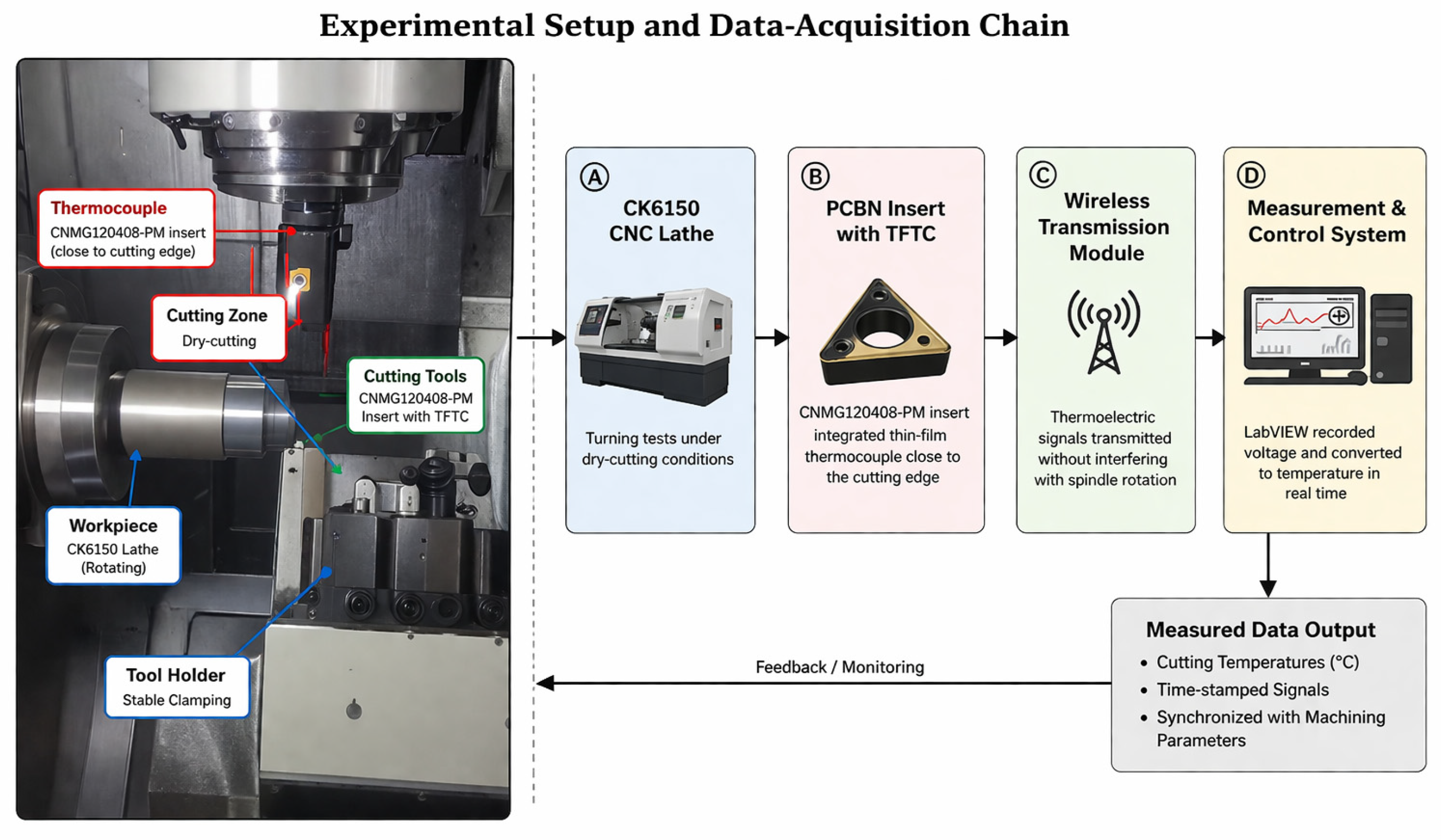
The workpiece protrusion length from the chuck was fixed at 30 mm (i.e., the cutting zone length). The remaining portion was supported by the tailstock centre of the lathe to further enhance stability during high-speed rotation (no noticeable vibration occurred at a cutting condition corresponding to a spindle speed of 2000 rpm). The physical diagram of the CK6150 CNC lathe experimental setup is shown in Figure 4.

The cutting tool system consisted of a PCBN insert (CNMG120408-PM) (Manufactured by Kyocera Corporation in Kyoto, Japan) mounted on a 25 mm × 25 mm × 150 mm tool holder. The thin-film thermocouple was positioned on the rake face at a distance of 0.5 mm from the main cutting edge, and the lead wires were routed through the holder to reduce mechanical interference during machining.

The PCBN tool (CNMG120408-PM) with integrated NiCr/NiSi thin-film thermocouple was mounted into the matching tool holder (25 mm × 25 mm × 150 mm) and secured via the holder’s locking screw (tightening torque 5 N·m) to prevent tool loosening.

The lathe turret’s automatic positioning function (repeat positioning accuracy: ±0.005 mm) was used to adjust the tool height. The cutting edge was aligned with the workpiece axis on the same horizontal plane with a height difference not exceeding 0.01 mm to prevent additional bending moments during cutting.

The mounting accuracy of the tool’s rake angle (−5°) and clearance angle (11°) was calculated. Using a tool presetter, the cutting edge was positioned 0.5 mm from the hot end of the thin-film thermocouple, consistent with design specifications.

Finally, the tool signal lead-out wire was routed through the reserved hole inside the tool holder and covered externally with high-temperature resistant insulating tubing to prevent entanglement or friction with the spindle or workpiece during cutting. The end of the signal transmission line was connected to the wireless transmission module fixed to the non-rotating section of the turret.

The workpiece material used throughout the study was AISI 1045 steel in the form of a solid cylindrical bar. The main dimensions and preparation tolerances are summarised below to facilitate reproduction of the tests.

The specimen had an overall length of 100 mm, a cutting section length of 30 mm and a nominal diameter of 50 mm. The end faces were prepared to maintain good perpendicularity relative to the axis, and the outer surface finish was controlled to ensure stable clamping and cutting conditions.

The same dimensional specification was adopted for all tests so that the influence of spindle speed and cutting time could be compared under consistent geometric conditions.

The core cutting component was a PCBN insert instrumented with the thin-film thermocouple. The insert geometry, tool reference and holder dimensions are given in

Table 2. Basic tool parameters (dry turning, cutting depth 0.5 mm, feed rate 0.1 mm/rev).

Item	Parameter Value
Tool Model	CNMG120408-PM
Material	Polycrystalline Cubic Boron Nitride (PCBN)
Tool Holder Size	25 mm × 25 mm × 150 mm
Insert Size	12 mm × 12 mm × 4.8 mm
Thin-Film Thermocouple Position	0.5 mm from the cutting edge on the rake face
Internal Drilling	Yes (for embedding cold junction or signal leads)

.

Specifically, the insert reference was CNMG120408-PM, with a nose radius of 0.8 mm, a rake angle of −5° and a clearance angle of 11°. These parameters were kept constant throughout the study.

The sensing region was arranged on the rake face close to the cutting edge so that the measured temperature would be sensitive to the thermal load generated at the tool–chip interface.

The thin-film thermocouple itself was fabricated on an Al₂O₃ substrate using NiCr and NiSi thermoelectric layers together with a SiO₂ protective layer, as described in Section 3.1.

The tool holder provided both mechanical clamping and electrical routing for the sensor leads.

An internal hole was reserved in the holder for signal transmission so that the wiring remained protected and did not affect chip flow or operator safety during the cutting tests.

The measurement system combined temperature acquisition, tool-wear observation and inverse heat-flux calculation. Temperature signals were collected through an NI cDAQ-9178/NI 9219 system (NI-DAQmx 2023 Q1), VB was measured after machining using a Keyence VHX-7000 microscope (The Keyence VHX-7000 microscope is manufactured by Keyence Corporation, Osaka, Japan.), and the recorded temperature history was used as input to the inverse numerical model.

To complete the thermocouple circuit, the tool holder was internally drilled to accommodate the cold junction and signal transmission lines, enabling stable thermoelectric signal collection. A wireless transmission module was integrated into the system to enable real-time monitoring of the cutting temperature without interfering with the machining process [9].

I.

Essential Equipment for Temperature-Related Measurements

The thin-film thermocouple signal acquisition device consisted of an NI cDAQ-9178 data acquisition card (National Instruments, Austin, TX, USA) and an NI 9219 thermocouple input module. With a sampling rate of 1000 Hz and a resolution of 0.001 mV, the system captured the thermoelectric-potential signal of the NiCr/NiSi thin-film thermocouple, while LabVIEW carried out real-time filtering and temperature conversion using the static calibration curve (R² = 0.998), so that the junction-temperature error did not exceed ±3.2 °C.

The dynamic response test device employed an Nd:YAG pulsed laser (Model CL532-100 (CVI Melles Griot, Carlsbad, CA, USA), wavelength 532 nm, pulse width 10 ns, energy 100 mJ) to provide laser-pulse excitation and simulate transient thermal shock during cutting. A high-speed infrared thermometer (Model OS3000, Omron Corporation, Kyoto, Japan, measurement range −20 to 1000 °C, response time 0.1 ms) was used simultaneously to verify that the 90% response time of the thin-film thermocouple was 0.49 s.

The cold-junction temperature control device was a high-precision constant-temperature bath (Model HWC-600, Hot Water Controls, Tulsa, OK, USA, control range 0–100 °C, control accuracy ±0.1 °C). The cold junction was fixed in the bath and maintained at 25 °C in order to eliminate the influence of ambient-temperature fluctuations on the thermoelectric-potential measurement.

II.

Heat Flux and Temperature Field Measurement/Calculation System

The IHCP inversion calculation system combined a three-dimensional thermal-conduction finite-element model of the tool established in ANSYS APDL 19.0 with a self-developed MATLAB R2022b IHCP solver integrating the SFS method and the future-time regularisation algorithm. The temperature data measured by the thin-film thermocouple were then used to invert the heat-flux density at the tool–chip interface, and the inversion time for a single dataset was kept below 3 min by using an Intel Core i9-13900K workstation.

The temperature-field verification device used a micro-thermocouple array (Omega TT-T-36-SLE, Omega Engineering, Stamford, CO, USA, wire diameter 0.1 mm, measurement range −50 to 750 °C). Thermocouples were embedded at depths of 0.5, 1, 3, and 5 mm inside the tool so that the internal temperature distribution could be measured and compared with the temperature field reconstructed by the IHCP inversion.

III.

Tool Wear and Sensor Performance Measurement Devices

The tool-wear measurement device for the VB value was a Keyence VHX-7000 ultra-depth-of-field 3D microscope (Carl Zeiss, Oberkochen, Germany) with a magnification range of 100–5000× and a measurement accuracy of ±0.1 μm. After the cutting experiments, the worn tool surface was scanned and imaged, and the built-in software (Windows 11 23H2) automatically identified the wear boundary to calculate the VB value.

The sensor performance was evaluated using the following test setup.

The static calibration device was a high-precision blackbody furnace (Model SR600, Stanford Research Systems (SRS), Sunnyvale, CA, USA, temperature-control range 50–1200 °C, control accuracy ±0.5 °C), which provided standard temperature points for calibrating the temperature-potential relationship of the thin-film thermocouple.

The interference-resistance test apparatus consisted of a high-frequency signal generator (Agilent 33220A, Agilent, Santa Clara, CA, USA, output frequency 10–20 MHz, amplitude 0–10 V) and an oscilloscope (Tektronix MDO3024, Tektronix, Beaverton, OR, USA, bandwidth 200 MHz, sampling rate 2.5 GS/s). This setup simulated industrial electromagnetic interference and monitored the output noise of the sensor, which remained within ±0.04 mV.

The thermal-shock durability test apparatus used a high–low temperature shock chamber (Model TS-408, QNAP, Taipei, China), temperature range −40 to 300 °C, switching time ≤ 5 s) to impose cyclic thermal shocks from 25 °C to 300 °C for 1000 cycles. A Fluke 8846A multimeter was used to monitor the thermoelectric-potential drift during the test.

The cutting-parameter control device was the CK6150 CNC lathe (Shenyang Machine Tool (Group) Co., Ltd., Shenyang, China), which precisely controlled the spindle speeds of 1000, 1500, and 2000 rpm together with a cutting depth of 0.5 mm and a feed rate of 0.1 mm/rev. The cutting durations of 30, 60, and 90 s were controlled by the built-in time relay so that the cutting parameters remained consistent throughout the experiments.

The workpiece and tool condition were monitored throughout the experiments.

A hardness tester (Model HV-1000, Mitutoyo Corporation, Kawasaki, Japan, test force 100–1000 g) was used to measure the initial hardness of the AISI 1045 steel workpiece, which ranged from HB 197 to HB 241. In addition, a Mitutoyo SJ-210 roughness tester (measurement range 0.01–100 μm, measurement accuracy ±0.001 μm) was used to verify that the pretreated tool surface roughness was Ra ≤ 0.05 μm before film deposition.

As shown in

Table 3. Cutting condition settings (dry turning, cutting depth 0.5 mm, feed rate 0.1 mm/rev).

Item	Setting Value
Workpiece Material	AISI 1045 steel
Spindle Speed (used here to denote the corresponding cutting-speed setting)	1000/1500/2000 rpm
Cutting Depth	0.5 mm
Feed Rate	0.1 mm/rev
Cutting/Lubrication Method	Dry cutting
Cutting Time	30 s/60 s/90 s
Cutting Speed	157/235.5/314 m/min

, AISI 1045 steel was selected as the workpiece material, with all experiments conducted under dry cutting conditions. The controlled variables were the cutting condition corresponding to spindle speeds of 1000, 1500 and 2000 rpm and cutting time (30, 60 and 90 s), while cutting depth and feed rate were held constant at 0.5 mm and 0.1 mm/revolution, respectively.

This study focuses on the dry turning of AISI 1045 steel using a PCBN tool instrumented with a thin-film thermocouple. The investigated cutting parameters correspond to spindle speeds of 1000–2000 rpm, cutting times of 30–90 s and a constant cutting depth of 0.5 mm. The analysis addresses the tool temperatures of 342–488 °C measured under these conditions, together with the friction and transient thermal loading at the tool–chip interface. Because PCBN is more commonly applied to hardened ferrous materials, the present results should be interpreted as an exploratory study of temperature monitoring and wear evolution under the selected dry-cutting condition rather than as an optimised industrial application case.

In

Table 4. Temperature-dependent mechanical and thermal properties of the principal materials at 25 °C and 450 °C (dry turning, cutting depth 0.5 mm, feed rate 0.1 mm/rev).

Material Name	Main Ingredients	Hardness (HV)	Melting Point/Maximum Operating Temperature (°C)	Coefficient of Thermal Expansion (×10−6/°C)	Thermal Conductivity (W/(m·K))
AISI 1045 steel	C 0.42–0.50%, Fe balance	200 (25 °C)/180 (450 °C)	1495	11.5 (25 °C)/13.2 (450 °C)	55 (25 °C)/48 (450 °C)
PCBN cutting tools	CBN particles + binder	3500 (25 °C)/3200 (450 °C)	1400	4.8 (25 °C)/5.5 (450 °C)	100 (25 °C)/110 (450 °C)
Thermocouple NiCr	Ni 80%, Cr 20%	220 (25 °C)/200 (450 °C)	1450	13.0 (25 °C)/14.2 (450 °C)	17 (25 °C)/20 (450 °C)
Thermocouple NiSi	Ni 97%, Si 3%	180 (25 °C)/160 (450 °C)	1410	11.0 (25 °C)/12.5 (450 °C)	25 (25 °C)/28 (450 °C)
Substrate Al2O3	Al2O3 (99.999%)	1800 (25 °C)/1750 (450 °C)	2054	7.5 (25 °C)/8.2 (450 °C)	30 (25 °C)/35 (450 °C)
Protective layer SiO2	SiO2	850 (25 °C)/800 (450 °C)	1713	0.5 (25 °C)/0.8 (450 °C)	1.4 (25 °C)/1.6 (450 °C)

, the values listed at 25 °C and 450 °C represent room-temperature and elevated-temperature properties, respectively. These temperature-dependent data were used as material-property inputs for the thermal analysis, where applicable and are also provided to characterise the materials within the investigated cutting-temperature range.

Throughout the cutting process, the measurement system simultaneously recorded the hot- and cold-junction temperatures, the thermoelectric potential and the tool wear (VB) value [35].

To ensure the reliability and accuracy of the thin-film thermocouple sensor, a comprehensive performance evaluation was carried out, including static calibration, dynamic response assessment, anti-interference testing and durability verification.

4.2. Correlation Analysis Between Cutting Temperature and Process Parameters

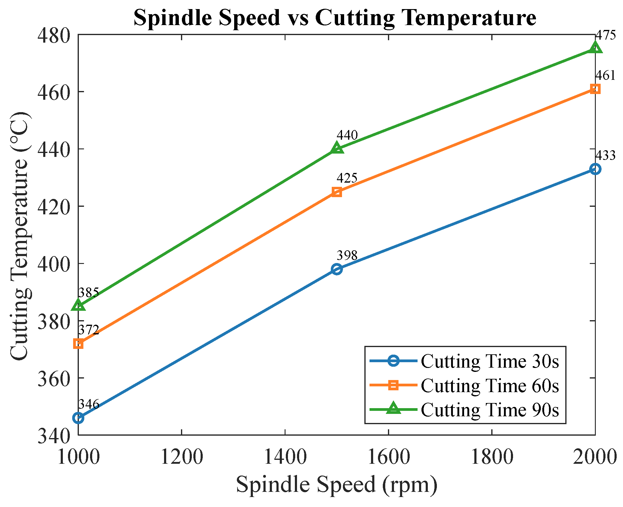
The numerical values summarised in

Table 5. Tool temperature measurement experimental data (dry turning, cutting depth 0.5 mm, feed rate 0.1 mm/rev).

No.	Spindle Speed (rpm; Corresponding Cutting-Speed Setting)	Cutting Time (s)	Hot Junction Temperature (°C)	Cold Junction Temperature (°C)	Thermoelectric Potential (mV)
T1	1000	30	342	25	1.46
T2	1000	60	368	25	1.63
T3	1500	30	382	25	1.71
T4	1500	60	405	25	1.82
T5	2000	30	428	25	1.93
T6	2000	60	445	25	2.01
T7	2000	90	466	25	2.11

and

Table 6. Temperature measurement results of tools integrated with thin-film thermocouples (dry turning, cutting depth 0.5 mm, feed rate 0.1 mm/rev).

No.	Spindle Speed (rpm; Corresponding Cutting-Speed Setting)	Cutting Time (s)	Maximum Temperature (°C)	Average Temperature (°C)	Temperature Rise Rate (°C/s)	Thermoelectric Potential (mV)	Tool Wear VB (mm)
M1	1000	30	346	324	10.7	1.48	0.082
M2	1000	60	373	352	5.8	1.65	0.135
M3	1500	30	389	370	13.4	1.75	0.119
M4	1500	60	418	396	7.2	1.88	0.181
M5	2000	30	437	421	17.0	1.98	0.172
M6	2000	60	462	443	7.0	2.10	0.237
M7	2000	90	488	468	5.0	2.23	0.295

, and the trends shown more clearly in Figure 5 and Figure 6, indicate that cutting temperature increased markedly with cutting speed. At a fixed cutting time of 30 s, increasing the cutting speed from 157 m/min to 314 m/min (corresponding to spindle speeds of 1000 rpm and 2000 rpm for the given workpiece diameter) raised the measured temperature from 342 °C to 428 °C. This result is consistent with the expected increase in frictional and plastic-deformation heat generation at the tool–chip interface.

These trends are consistent with the findings reported in [35,36,37,38], where higher tool-rotation speed was also associated with higher interface temperature. In the present turning tests, the observed temperature rise at higher cutting speed is therefore attributed to the increased conversion of mechanical energy into frictional and plastic-deformation heat at the tool–workpiece interface.

The relationship between cutting speed (reported through the corresponding spindle speed setting) and cutting temperature is shown in Figure 5.

Figure 6 illustrates the influence of cutting speed and cutting time on cutting temperature for AISI 1045 steel under dry turning conditions. As the cutting speed increased from 157 m/min to 314 m/min, the cutting temperature showed a clear upward trend. At the same time, longer cutting duration led to additional heat accumulation in the insert-workpiece system. The corrected figure description therefore refers to the combined effect of cutting speed and cutting time, not to spindle speed alone.

Influence of Cutting Time on Cutting Temperature

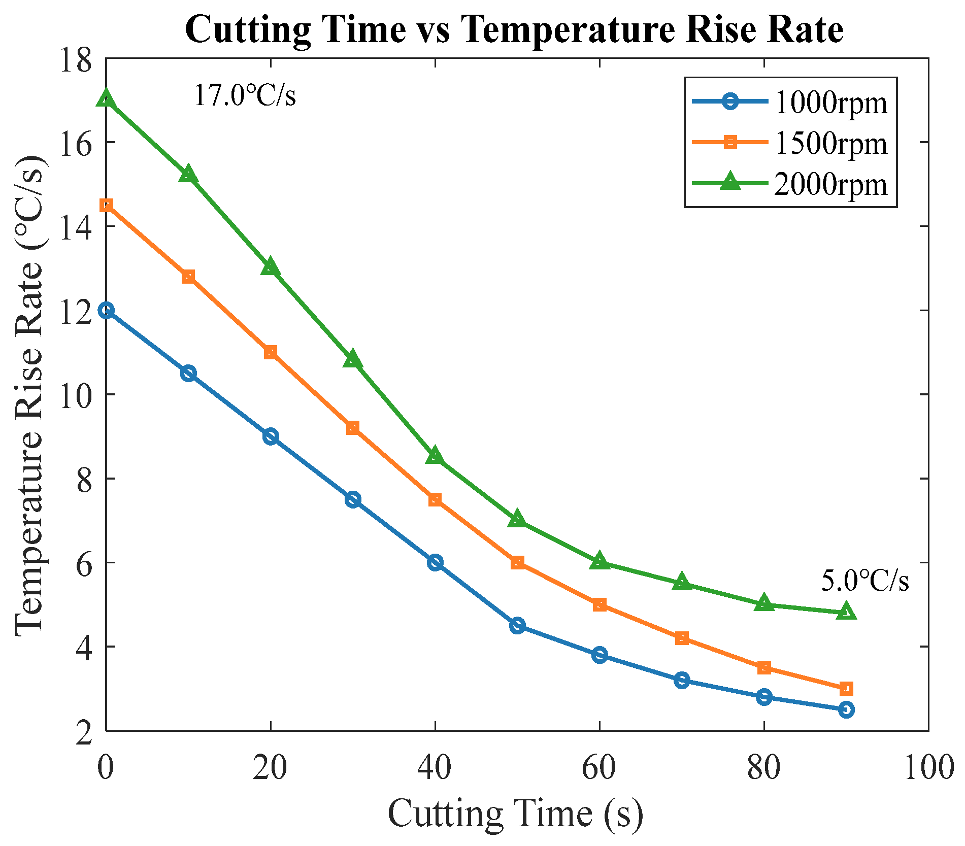
At a fixed spindle speed, the temperature also increased with cutting time, although the rate of increase gradually decreased as the tool approached a thermal quasi-steady state. The graphical trend in Figure 6 is therefore used as the main basis for discussion, while the corresponding tables are retained only to provide the original numerical values. The 90 s condition is reported only for the highest spindle-speed condition because this was the most thermally severe case selected for the extended verification test; the lower-speed conditions were limited to shorter durations in the comparative dataset shown in the tables.

Thermoelectric potential increased synchronously with spindle speed (1.46–1.63 mV at 1000 rpm, 1.93–2.11 mV at 2000 rpm), with a deviation of less than 3% from the values calculated by the Seebeck effect formula (SAB = (V1 − V2)/(T1 − T0)). This indicates the stable thermoelectric conversion performance of the Ni-Cr/Ni-Si thin-film thermocouples (1200 nm). The relationship between cutting time and temperature rise rate is shown in Figure 6.

Figure 6 illustrates how the temperature rise rate varies with cutting time under the three tested cutting conditions. During the initial phase (0–30 s), the heating rate is highest because the tool and workpiece have not yet reached thermal equilibrium. As cutting continues, heat conduction into the PCBN insert and the workpiece reduces the temperature-rise rate, so the curves gradually flatten with time.

Unlike the response lag typically observed in conventional thermocouples, the thin-film thermocouple demonstrated stable output during 90 s of continuous cutting. The hot-junction temperature reached 466 °C, and the corresponding thermoelectric potential measured 2.11 mV. The deviation between the maximum and average temperatures remained below 5%, indicating excellent measurement stability. These results confirm that the 1000 nm SiO₂ protective layer effectively minimised damage to the thermoelement films caused by chip–tool friction, thereby ensuring reliable sensor performance during prolonged cutting tests. Selecting the typical operating condition of “2000 rpm spindle speed + 60 s cutting time” for case analysis.

Real-time temperature signal recording examples are shown in

Table 7. Example of real-time temperature signal recording (dry turning, cutting depth 0.5 mm, feed rate 0.1 mm/rev).

Timepoint (s)	Hot-End Temperature (°C)	Cold-End Temperature (°C)	Thermal EMF (mV)	Note
0 (Cutting begins)	25.3	25.0	0.01	The tool has not contacted the workpiece; its temperature matches the ambient temperature.
5	186.7	25.1	0.82	The tool and workpiece make initial contact, causing the temperature to rise rapidly.
15	324.5	25.0	1.43	Cutting heat accumulates rapidly, accelerating the rate of temperature rise.
30	412.3	25.1	1.85	Temperature has entered a phase of rapid increase, approaching the peak range.
45	451.6	25.0	2.04	The rate of temperature increase is slowing down and gradually approaching a stable state.
60 (Cutting complete)	462.1	25.1	2.10	Reach the maximum temperature under this operating condition

.

4.3. Correlation Verification Between Tool Wear and Cutting Temperature

Correlation analysis revealed a strong positive relationship between tool wear (VB) and cutting temperature. The coefficient of determination (R² = 0.97) was obtained from a least-squares linear regression between the mean maximum cutting temperature and the mean VB value for each cutting condition. VB was measured from microscope images after machining, and the temperature values were taken from the thin-film thermocouple records. This statistical result supports a strong association within the tested parameter window, but it should not be interpreted as proof of a one-way causal mechanism.

For each cutting condition, three repeated turning tests were carried out and the average VB value was used in the regression analysis; the standard deviation and coefficient of variation are reported in

Table 8. VB value (tool wear) variability (dry turning, cutting depth 0.5 mm, feed rate 0.1 mm/rev).

Cutting Conditions (Rotational Speed/Time)	3 Repeat VB Values (mm)	Average Value (mm)	Standard Deviation (mm)	Coefficient of Variation (CV%)
1000 rpm/30 s	0.080, 0.082, 0.084	0.082	0.002	2.44
1000 rpm/60 s	0.132, 0.135, 0.138	0.135	0.003	2.22
1500 rpm/30 s	0.117, 0.119, 0.121	0.119	0.002	1.68
1500 rpm/60 s	0.178, 0.181, 0.184	0.181	0.003	1.66
2000 rpm/30 s	0.170, 0.172, 0.174	0.172	0.002	1.16
2000 rpm/60 s	0.234, 0.237, 0.240	0.237	0.003	1.27
2000 rpm/90 s	0.292, 0.295, 0.298	0.295	0.003	1.02

to document repeatability.

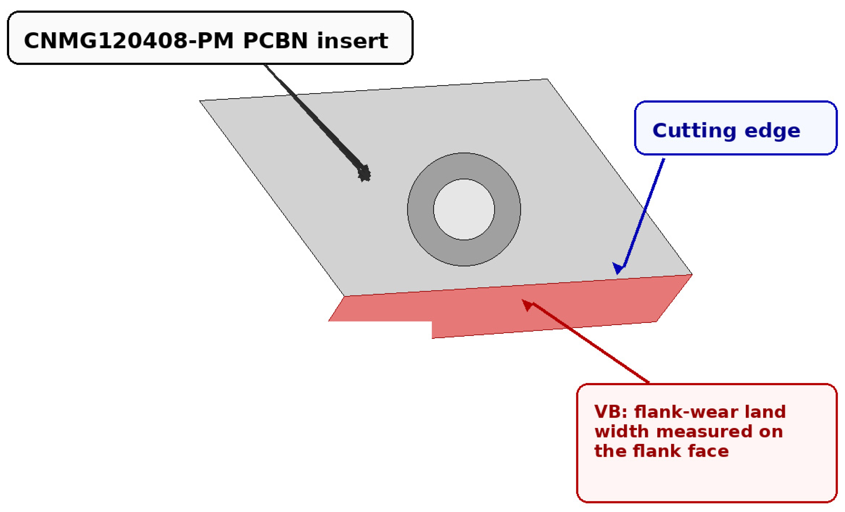
Figure 7 presents the CNMG120408-PM PCBN cutting insert used in the turning experiments and explicitly indicates the flank-wear land width VB measured on the flank face. The revised figure was added to identify both the tool type and the wear definition more clearly.

Under all operating conditions, the coefficient of variation for the VB value did not exceed 2.44%, indicating overall low variability and good experimental repeatability.

Under low-speed and short-cutting-time conditions (e.g., 1000 rpm/30 s), the coefficient of variation is slightly higher than under high-speed and long-cutting-time conditions. This is primarily because the initial wear amount is small (not exceeding 0.1 mm), making it more significantly affected by differences in the initial micro-morphology of the tool edge.

As cutting time increases and wear accumulates, the coefficient of variation gradually decreases (e.g., CV = 1.02% at 2000 rpm/90 s). This occurs because tool wear enters a stable phase, leading to more consistent cutting edge conditions and reducing the influence of initial variations.

The standard deviation of the hot-end temperature across the three repeated experiments within each group was no more than ±3.5 °C, and the corresponding coefficient of variation was no more than 0.82%, indicating low variability of the temperature measurements.

The thermocouple electromotive force also showed good repeatability, with a standard deviation no greater than ±0.02 mV and a coefficient of variation no greater than 0.98%, which confirms the stable thermoelectric-conversion performance of the NiCr/NiSi thin-film thermocouple electrodes.

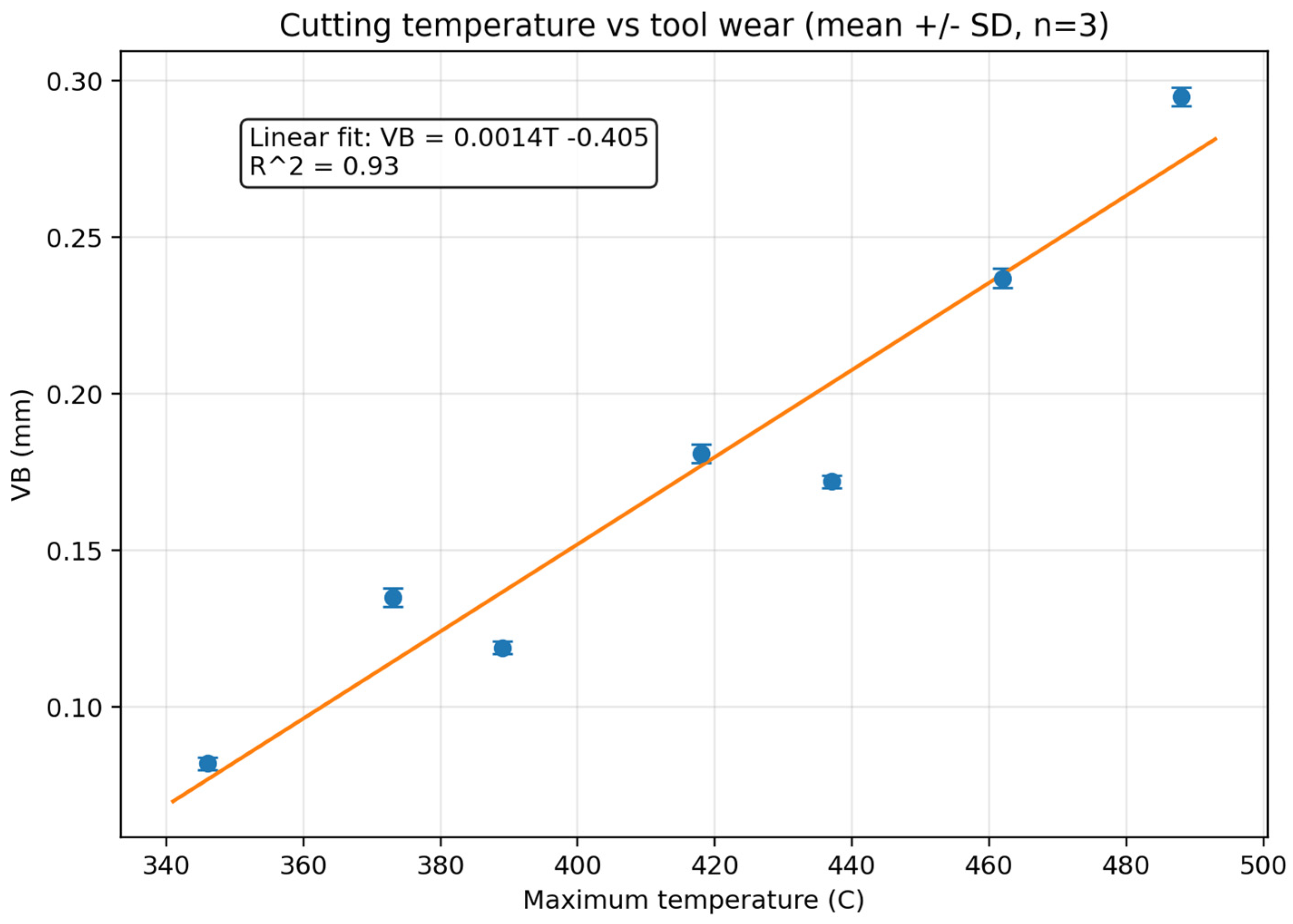
As the maximum temperature increased from 346 °C (M1) to 488 °C (M7), the VB value increased from 0.082 mm to 0.295 mm (see Table 6), showing a strong positive association between cutting temperature and flank wear under the investigated conditions. To assess repeatability, three repeated tests were performed for each condition, and the results shown in Figure 8 were plotted as mean values with standard deviation error bars.

The observed wear behaviour is interpreted in relation to the selected material pair and dry-cutting condition. In the present dry turning of non-heat-treated AISI 1045 steel with PCBN, the increase in wear at higher temperature and cutting speed is discussed more cautiously as the combined effect of adhesion, diffusion/chemical interaction and oxidation at the tool–workpiece interface, together with the larger mechanical and thermal load at higher cutting speed. This interpretation is also consistent with literature reporting that temperature rise, contact stress and wear evolution interact simultaneously during cutting rather than through a single isolated mechanism.

Figure 8 summarises the relationship between maximum cutting temperature and flank wear VB for the dry turning tests performed at spindle speeds of 1000, 1500, and 2000 rpm and cutting times of 30, 60, and 90 s, with a cutting depth of 0.5 mm and a feed rate of 0.1 mm/rev. Each point represents the mean value of three repeated experiments, and the error bars denote the standard deviation. The small dispersion indicates that the three repeated experiments were close to each other, although they were not exactly identical.

4.4. Performance Verification of Thin-Film Thermocouple Sensors

4.4.1. Static Accuracy and Dynamic Response

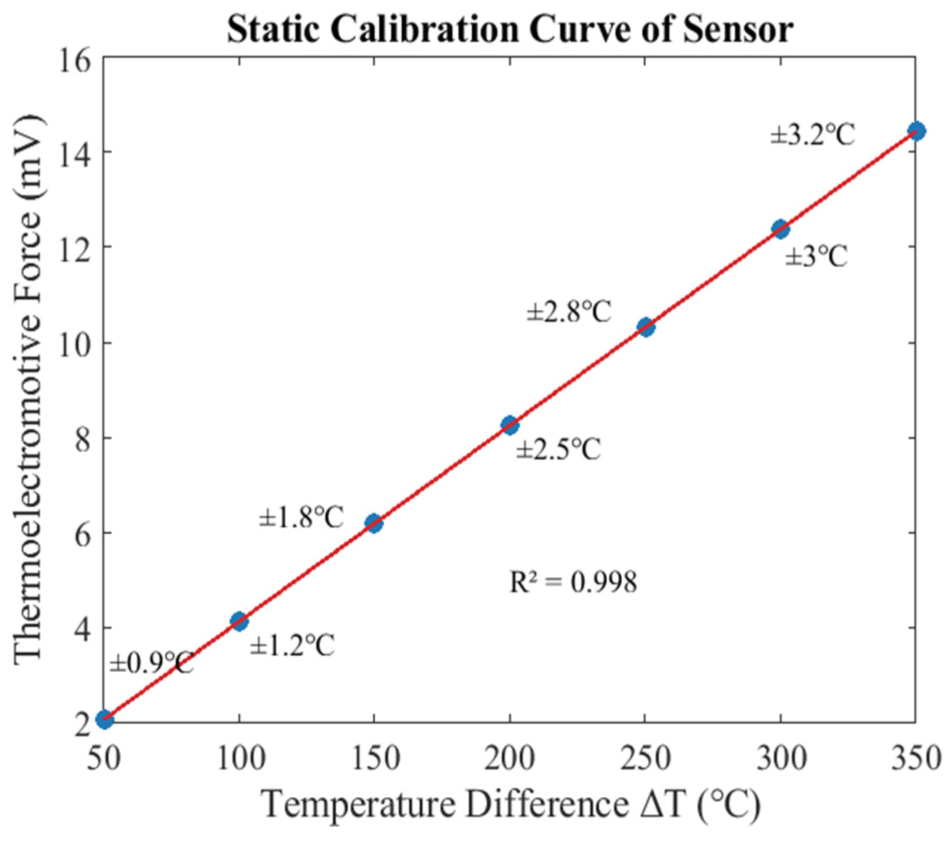
Static calibration results (

Table 9. Static test data (temperature-potential calibration, dry turning, cutting depth 0.5 mm, feed rate 0.1 mm/rev).

Test No.	Hot Junction Temperature (°C)	Cold Junction Temperature (°C)	Temperature Difference ΔT (°C)	Thermoelectric Potential Output (mV)	Nominal Error (°C)
S1	50	25	25	1.15	±0.9
S2	100	25	75	3.42	±1.2
S3	150	25	125	5.79	±1.6
S4	200	25	175	8.15	±2.1
S5	250	25	225	10.50	±2.5
S6	300	25	275	12.82	±2.8
S7	350	25	325	15.16	±3.2

) showed a linear relationship between thermoelectric potential and temperature difference (ΔT) in the range of 50–350 °C (R² = 0.998), with a nominal error of ±0.9~±3.2 °C. This outperforms sensors prepared by the sol–gel method (error > ±5 °C), verifying the high-precision advantage of magnetron-sputtered films (density, uniformity).

The static calibration curve of the sensor is shown in Figure 9.

Figure 9 shows the “temperature difference–thermocouple voltage” calibration curve for the thin-film thermocouple sensor. The linear fit R² = 0.998 indicates a highly linear relationship between the sensor output signal and temperature difference. Furthermore, the nominal error at each temperature point does not exceed ±3.2 °C, meeting the accuracy requirements for cutting temperature measurement. This further validates the sensor’s reliable performance under static operating conditions.

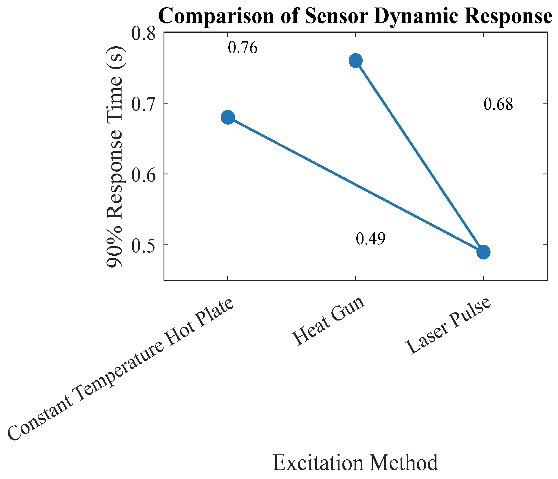
Dynamic response tests (

Table 10. Dynamic response test data (response speed and hysteresis, dry turning, cutting depth 0.5 mm, feed rate 0.1 mm/rev).

Test No.	Method	Step Temperature (°C)	Time to 90% Response (s)	Time to 95% Response (s)	Response Characteristics
D1	Heat Gun	25→200	0.65	0.81	No overshoot, fast stabilisation
D2	Heat Gun	25→300	0.61	0.79	Micro-fluctuation (±0.02 mV)
D3	Laser Pulse	25→250	0.49	0.68	Low jitter, low hysteresis
D4	Constant Temperature Hot Plate	25→150	0.76	0.92	Smooth response curve

) showed a time to 90% response of only 0.49 s under laser-pulse excitation (25→250 °C) with no significant overshoot. In Table 10, D1 and D2 denote heat-gun step-heating tests, D3 denotes the laser-pulse test, and D4 denotes the constant-temperature hot-plate test. These four test numbers were used to compare the response speed and stability of the sensor under different thermal excitation modes.

The dynamic response of the sensor is illustrated in Figure 10.

Figure 10 compares the 90% response times of the sensor under three excitation methods: laser pulse excitation yields the shortest response time at just 0.49 s, while the thermal gun and constant-temperature hot plate exhibit relatively longer response times of 0.76 s and 0.68 s, respectively. This result demonstrates that the sensor can rapidly capture transient temperature changes during cutting operations, making it suitable for “cut-in/cut-out” transient thermal shock scenarios in dry cutting processes.

4.4.2. Stability and Anti-Interference

Repeatability tests (see

Table 11. Repeatability and drift test data (dry turning, cutting depth 0.5 mm, feed rate 0.1 mm/rev).

Cycle Range	Average Output (mV)	Deviation Range (mV)	Drift Percentage (%)
1–10	8.15	±0.03	0.37%
11–50	8.14	±0.04	0.49%
51–100	8.12	±0.05	0.61%

) showed an output deviation of ≤±0.05 mV (drift rate: 0.61%) over 100 cycles, which is much lower than the 1.5% drift rate of electroplated sensors. This confirms that the bonding force between the NiCr/NiSi films and the substrate ensures long-term stability (the adhesion strength between NiCr/NiSi thermoelectric electrode films and Al₂O₃ substrates is 18.6 ± 1.2 N. The adhesion strength between the SiO₂ protective layer and NiCr/NiSi electrode films is 16.3 ± 1.5 N. Both values were quantitatively characterised using the scratch test method.).

Anti-interference tests (

Table 12. Anti-interference test data (dry turning, cutting depth 0.5 mm, feed rate 0.1 mm/rev).

Condition	Input Temperature Difference (°C)	Output Signal (mV)	Noise Amplitude (mV)	Drift
Normal Environment	175	8.15	±0.01	No
Near Welding Machine	175	8.13	±0.03	No
High-Frequency Interference Source	175	8.11	±0.04	No
Abnormal Grounding	175	7.98	±0.07	Slight

) showed that in environments with welding machines and high-frequency interference sources, the output noise amplitude was ≤±0.04 mV, with only slight drift (7.98 mV) under abnormal grounding. This indicates the effective electromagnetic compatibility design of the wireless signal transmission system, meeting the requirements of industrial field applications.

Anti-interference tests (Table 12) further confirmed that the sensor output remained stable under common industrial electromagnetic disturbances, with only limited drift under abnormal grounding conditions.

4.4.3. Thermal Shock Durability

After 1000 thermal shock cycles (25→300 °C), the sensor showed a thermoelectric potential drift of 2.8% and a resistance change rate of 5.6%, with only slight microcracks (

Table 13. Thermal shock durability test data (dry turning, cutting depth 0.5 mm, feed rate 0.1 mm/rev).

Cycle Number	Thermoelectric Potential Drift (%)	Resistance Change Rate (%)	Appearance Defects
0	0%	0%	None
500	1.6%	3.4%	None
1000	2.8%	5.6%	Slight microcracks, no peeling

). Combined with the “strong film–substrate bonding” of magnetron sputtering, this confirms the sensor’s ability to withstand thermal stress impacts in complex cutting environments, meeting the service life requirements of mass production.

From a measurement-reliability perspective, the repeated tests reported in Table 8, Table 9, Table 10, Table 11, Table 12 and Table 13 indicate low dispersion of VB, temperature and thermoelectric voltage. These repeatability data provide an initial error estimate for the present study. Although a more comprehensive uncertainty budget and ANOVA-based factor analysis should be developed in future work, the current dataset is sufficiently consistent to support the comparative discussion of temperature and wear trends.

The experimental results demonstrate that the Ni-Cr/Ni-Si thin-film thermocouple, which was produced using magnetron sputtering technology, enables precise temperature measurement during cutting with an error margin of less than 3.2 °C. It also has a fast response time of less than 0.5 s, strong anti-interference capabilities and a long durability of 1000 cycles. The quantitative relationships between cutting temperature and spindle speed/cutting time (Section 4.2) provide a basis for optimising process parameters, while the strong correlation between temperature and tool wear (Section 4.3) forms the basis for constructing a tool life prediction model.

The sensor’s performance advantages stem from the selection and preparation of materials: the high-purity Al₂O₃ insulation film (1500 nm) prevents thermoelectric-potential shunting, the SiO₂ protective film (1000 nm) improves wear resistance, and the dense magnetron-sputtered film structure helps reduce thermal hysteresis. However, the experiments were limited to dry turning of AISI 1045 steel; therefore, applicability to hardened steels or other difficult-to-cut materials remains to be verified in future work.

4.5. Validation of IHCP Inversion Results

Based on the IHCP inversion, the transient heat flux at the tool–chip interface was reconstructed from the measured temperature history and then compared with the corresponding temperature rise and tool-wear evolution. The numerical results, therefore, complement the experimental observations by providing a physically interpretable estimate of the thermal load acting on the tool during cutting.

Table 14. Heat-flux density, temperature, and tool-wear data (dry turning, cutting depth 0.5 mm, feed rate 0.1 mm/rev).

Experiment Number	Cutting Parameters (Rotational Speed/Time)	Inverted Heat Flux Density $\mathit{q}$(MW/m2)	Maximum Tool Temperature ${\mathit{T}}_{\mathbf{max}}$ (°C)	Thermal Softening Coefficient ξ	Wear Amount VB (mm)	Model Prediction VB (mm)	Relative Error (%)
M1	1000 rpm/30 s	5.5	346	0.89	0.082	0.079	3.7
M2	1000 rpm/60 s	8.7	373	0.83	0.135	0.128	5.2
M3	1500 rpm/30 s	10.3	389	0.80	0.119	0.114	4.2
M4	1500 rpm/60 s	13.1	418	0.74	0.181	0.175	3.3
M5	2000 rpm/30 s	15.6	437	0.70	0.172	0.168	2.3
M6	2000 rpm/60 s	18.2	462	0.65	0.237	0.231	2.5
M7	2000 rpm/90 s	22.0	488	0.57	0.295	0.287	2.7

shows that higher interface heat flux was associated with higher measured temperature and larger VB values. Although the heat flux itself cannot be measured directly during turning, the inversion results followed the same trend as the experimental data, supporting the validity of the thermo-mechanical interpretation adopted in this study.

Notably, both heat flux density and wear volume reached their peaks during the extended cutting test (M7) at 2000 rpm for 90 s. This indicates that sustained heat accumulation accelerates oxidation, adhesion, and abrasive wear on the tool surface, resulting in a nonlinear increase in wear rate.

Further analysis revealed a high correlation between heat flux density and tool temperature trends, while a pronounced negative correlation existed between the decrease in thermal softening coefficient and temperature rise. This pattern indicates that heat flux density, as a direct reflection of cutting thermal load, is the core physical quantity driving tool wear. Additionally, this study established a tool wear prediction model by integrating heat flux density and thermal softening coefficient derived from IHCP inversion. The relative error between the model’s predictions and experimental measurements was consistently controlled within the range of 2.3% to 5.2%. This not only validates the effectiveness and accuracy of the IHCP method in obtaining cutting thermal boundary conditions but also demonstrates the model’s reliable applicability for tool wear monitoring and life prediction in actual machining processes. It provides a crucial theoretical basis and technical support for optimising cutting parameters, reducing production costs, and enhancing machining efficiency.

5. Conclusions

In this study, a homemade NiCr/NiSi thin-film thermocouple integrated with a PCBN cutting tool was developed for dry turning of AISI 1045 steel. The key contribution of the work is the establishment of a reproducible sensor-and-analysis framework in which the sensor structure, material selection, fabrication route, cutting tests and inverse thermal interpretation are reported together rather than separately. Under the investigated conditions corresponding to spindle speeds of 1000–2000 rpm, cutting times of 30–90 s, cutting depth of 0.5 mm and feed rate of 0.1 mm/rev, the system enabled real-time measurement of the hot-junction temperature close to the cutting edge.

The sensor exhibited good measurement performance, including a 90% dynamic response time of 0.49 s, acceptable repeatability and satisfactory resistance to interference and thermal shock. Experimentally, both cutting temperature and VB increased with cutting speed and cutting time, and regression analysis showed a strong positive temperature–wear correlation (R² = 0.97). This result should be interpreted as a statistically strong association within the studied parameter window rather than a stand-alone demonstration of causality.

The inverse heat-conduction analysis further showed that the reconstructed interface heat flux evolved consistently with the measured temperature and wear results, which supports the use of the proposed framework for thermo-mechanical interpretation of tool degradation. Accordingly, the principal scientific contribution of the present work is to demonstrate that a tool-integrated thin-film thermocouple can provide stable temperature data that are sufficiently reliable for combined experimental and inverse-analysis evaluation of temperature–wear behaviour in turning. Future work should include broader statistical analysis, additional wear-imaging datasets and extension to other workpiece materials and cutting conditions.

References

1. Santos, M.C.; Araújo Filho, J.S.; Barrozo, M.A.S.; Jackson, M.J.; Machado, A.R. Development and application of a temperature measurement device using the tool-workpiece thermocouple method in turning at high cutting speeds. Int. J. Adv. Manuf. Technol. 2017, 89, 2287–2298. [Google Scholar]
2. Absar, S.; Ruszkiewicz, B.J.; Skovron, J.D.; Mears, L.; Abke, T.; Zhao, X.; Choi, H. Temperature measurement in friction element welding process with micro thin film thermocouples. Procedia Manuf. 2018, 26, 485–494. [Google Scholar] [CrossRef]
3. Junge, T.; Liborius, H.; Mehner, T.; Nestler, A.; Schubert, A.; Lampke, T. Measurement system based on the Seebeck effect for the determination of temperature and tool wear during turning of aluminum alloys. Procedia CIRP 2020, 93, 1435–1441. [Google Scholar] [CrossRef]
4. Garcia, D.; Wang, T.; Escobar, J.D.; Pole, M.; Ma, X.; Ross, K.A. In-situ measurement and control of the tool-workpiece interface temperature during friction stir processing of 304/304L stainless steel. Mater. Today Commun. 2023, 38, 107672. [Google Scholar] [CrossRef]
5. Huang, S.; Tao, B.; Li, J.; Fan, Y.; Yin, Z. Estimation of the time and space-dependent heat flux distribution at the tool-chip interface during turning using an inverse method and thin film thermocouples measurement. Int. J. Adv. Manuf. Technol. 2018, 99, 1531–1543. [Google Scholar] [CrossRef]
6. Davoodi, B.; Hosseinzadeh, H. A new method for heat measurement during high speed machining. Measurement 2012, 45, 2135–2140. [Google Scholar] [CrossRef]
7. Chen, J.; Lin, Y.; Zhao, D.; Gao, S.; Zheng, M.; Ma, W.; Chen, B. Integrated design and fabricate of high sensitivity built-in thin-film thermocouple temperature measurement tool. J. Mech. 2024, 40, 110–120. [Google Scholar] [CrossRef]
8. Bharathi, S.J.; Thilagar, S.H. Heat Transfer Analysis on Platinum-Based Thin-Film Temperature Sensor Element for Liquid Temperature Measurement Applications. Heat Transf. Res. 2021, 52, 35–60. [Google Scholar] [CrossRef]
9. Zhao, G.; Li, X.; Liu, Z. Research on Precise Temperature Monitoring and Thermal Management Optimization of Automobile Engines Based on High-Precision Thin-Film Thermocouple Technology. Micromachines 2025, 16, 249. [Google Scholar] [CrossRef]
10. Kesriklioglu, S.; Morrow, J.D.; Pfefferkorn, F.E. Tool–Chip Interface Temperature Measurement in Interrupted and Continuous Oblique Cutting. J. Manuf. Sci. Eng. 2018, 140, 051013. [Google Scholar] [CrossRef]
11. Basti, A.; Obikawa, T.; Shinozuka, J. Tools with built-in thin film thermocouple sensors for monitoring cutting temperature. Int. J. Mach. Tools Manuf. 2007, 47, 793–798. [Google Scholar] [CrossRef]
12. Varga, J.; Demko, M.; Kaščák, Ľ.; Ižol, P.; Vrabeľ, M.; Brindza, J. Influence of Tool Inclination and Effective Cutting Speed on Roughness Parameters of Machined Shaped Surfaces. Machines 2024, 12, 318. [Google Scholar] [CrossRef]
13. Huang, S.; Tao, B.; Li, J.; Fan, Y.; Yin, Z. On-line estimation of the tool-chip interface temperature field during turning using a sequential inverse method. Int. J. Adv. Manuf. Technol. 2018, 97, 939–952. [Google Scholar] [CrossRef]
14. Li, J.; Tao, B.; Huang, S.; Yin, Z. Built-in thin film thermocouples in surface textures of cemented carbide tools for cutting temperature measurement. Sens. Actuators A Phys. 2018, 279, 663–670. [Google Scholar] [CrossRef]
15. Biermann, D.; Kirschner, M.; Pantke, K.; Tillmann, W.; Herper, J. New coating systems for temperature monitoring in turning processes. Surf. Coat. Technol. 2013, 215, 376–380. [Google Scholar] [CrossRef]
16. Garcia-Gonzalez, J.C.; Moscoso-Kingsley, W.; Madhavan, V. Tool Rake Face Temperature Distribution When Machining Ti6Al4V and Inconel 718. Procedia Manuf. 2016, 5, 1369–1381. [Google Scholar] [CrossRef]
17. Werschmoeller, D.; Li, X. Measurement of tool internal temperatures in the tool–chip contact region by embedded micro thin film thermocouples. J. Manuf. Process. 2011, 13, 147–152. [Google Scholar] [CrossRef]
18. Lian, Y.; Chen, X.; Zhang, T.; Liu, C.; Lin, L.; Lin, F.; Li, Y.; Chen, Y.; Zhang, M.; Zhou, W. Temperature measurement performance of thin-film thermocouple cutting tool in turning titanium alloy. Ceram. Int. 2022, 49, 2250–2261. [Google Scholar] [CrossRef]
19. Norouzifard, V.; Hamedi, M. A three-dimensional heat conduction inverse procedure to investigate tool–chip thermal interaction in machining process. Int. J. Adv. Manuf. Technol. 2014, 74, 1637–1648. [Google Scholar] [CrossRef]
20. Li, T.; Shi, T.; Tang, Z.; Liao, G.; Duan, J.; Han, J.; He, Z. Real-time tool wear monitoring using thin-film thermocouple. J. Mech. Work. Technol. 2021, 288, 116901. [Google Scholar] [CrossRef]
21. Bali, A.; Chetty, R.; Mallik, R.C. Thin film thermoelectric materials for sensor applications: An overview. In Thin Film Structures in Energy Applications; Springer: Cham, Switzerland, 2015; pp. 215–241. [Google Scholar] [CrossRef]
22. Kesriklioglu, S.; Pfefferkorn, F.E. Real time temperature measurement with embedded thin-film thermocouples in milling. Procedia CIRP 2018, 77, 618–621. [Google Scholar] [CrossRef]
23. Zendehnam, A.; Ghasemi, J.; Zendehnam, A. Employing cold atmospheric plasma (Ar, He) on Ag thin film and their influences on surface morphology and anti-bacterial activity of silver films for water treatment. Int. Nano Lett. 2018, 8, 157–164. [Google Scholar] [CrossRef]
24. Zhou, D.; Huang, L.; Yuan, J. Oxidation behaviour of NiSi–NiCr thin film thermocouples and antioxidation effect of SiNxOy film. Ceram. Int. 2024, 50, 25810–25821. [Google Scholar] [CrossRef]
25. Barrera, M.; Vogel, C.; Fietzke, F. Magnetron-sputtered thin films enabling heat transfer enhancement in electrocaloric heat pumps. Surf. Coat. Technol. 2025, 502, 131973. [Google Scholar] [CrossRef]
26. Liu, H.; Mao, X.; Jiang, S. Influence of substrate temperature on the microstructure of YSZ films and their application as the insulating layer of thin film sensors for harsh temperature environments. Ceram. Int. 2022, 48, 13524–13530. [Google Scholar] [CrossRef]
27. Liu, Y.; Jiang, H.; Zhao, X.; Deng, X.; Zhang, W. High temperature electrical insulation and adhesion of nanocrystalline YSZ/Al2O3 composite film for thin-film thermocouples on Ni-based superalloy substrates. Appl. Surf. Sci. 2022, 579, 152169. [Google Scholar] [CrossRef]
28. Ayes, A.; Bernhardt, G.; da Cunha, M.P. Removal of Stress Hillocks from Platinum-Alumina Electrodes Used in High-temperature SAW Devices. In Proceedings of the 2019 IEEE International Ultrasonics Symposium (IUS), Glasgow, UK, 6–9 October 2019; pp. 727–730. [Google Scholar]
29. Liu, H.; Mao, X.; Jiang, S. Effect of thermally grown Al2O3 on electrical insulation properties of thin film sensors for high temperature environments. Sens. Actuators A Phys. 2021, 331, 113033. [Google Scholar] [CrossRef]
30. Kim, J.H.; Jang, K.L.; Ahn, K.; Yoon, T.; Lee, T.I.; Kim, T.S. Thermal expansion behavior of thin films expanding freely on water surface. Sci. Rep. 2019, 9, 7071. [Google Scholar] [CrossRef]
31. Jianxin, D.; Tongkun, C.; Lili, L. Self-lubricating behaviors of Al2O3/TiB2 ceramic tools in dry high-speed machining of hardened steel. J. Eur. Ceram. Soc. 2005, 25, 1073–1079. [Google Scholar] [CrossRef]
32. Sinha, B.K.; Patel, M.S. Recent developments in high precision quartz and Langasite pressure sensors for high temperature and high pressure applications. In Proceedings of the 2016 IEEE International Frequency Control Symposium (IFCS), New Orleans, LA, USA, 9–12 May 2016; pp. 1–13. [Google Scholar]
33. Ren, Z.; Bin Mujib, S.; Singh, G. High-Temperature Properties and Applications of Si-Based Polymer-Derived Ceramics: A Review. Materials 2021, 14, 614. [Google Scholar] [CrossRef] [PubMed]
34. Kaseem, M.; Ko, Y.G. A novel hybrid composite composed of albumin, WO3, and LDHs film for smart corrosion protection of Mg alloy. Compos. Part B Eng. 2021, 204, 108490. [Google Scholar] [CrossRef]
35. Liu, X.; Han, K. Design of Temperature Monitoring and Fault Warning System for Lithium Ternary Battery Case. Micromachines 2025, 16, 345. [Google Scholar] [CrossRef] [PubMed]
36. Shi, X.L.; Zou, J.; Chen, Z.G. Advanced thermoelectric design: From materials and structures to devices. Chem. Rev. 2020, 120, 7399–7515. [Google Scholar] [CrossRef] [PubMed]
37. Wang, H. Research on NiCr/NiSi thin film thermocouple sensor for measuring the surface temperature of automobile engine. Front. Mater. 2025, 12, 1554564. [Google Scholar] [CrossRef]
38. Sengupta, P.; Bhattacharjee, A.; Maiti, H.S. Zirconia: A Unique Multifunctional Ceramic Material. Trans. Indian Inst. Met. 2019, 72, 1981–1998. [Google Scholar] [CrossRef]
Figure 1. Schematic diagram of temperature measurement principle of thin-film thermocouple.
Crystals 16 00312 g001
Figure 2. Schematic diagram of the thin-film thermocouple sample.
Crystals 16 00312 g002
Figure 3. Annotated view of the cutting tool showing the tool holder and the thin-film thermocouple region near the cutting edge.
Crystals 16 00312 g003
Figure 4. High-contrast view of the CK6150 CNC lathe experimental setup and data-acquisition chain with enlarged, readable labels.
Crystals 16 00312 g004
Figure 5. Relationship between cutting condition (corresponding spindle speed) and cutting temperature in dry turning of AISI 1045 steel at fixed cutting time.
Crystals 16 00312 g005
Figure 6. Effect of cutting time on the temperature rise rate under three cutting conditions corresponding to spindle speeds of 1000, 1500, and 2000 rpm in dry turning of AISI 1045 steel.
Crystals 16 00312 g006
Figure 7. CNMG120408-PM PCBN cutting insert used in the turning tests and definition of the flank-wear land width VB.
Crystals 16 00312 g007
Figure 8. Cutting temperature versus tool wear (VB value) with error bars from three repeated experiments.
Crystals 16 00312 g008
Figure 9. Static calibration curve of sensor.
Crystals 16 00312 g009
Figure 10. Comparison of sensor dynamic response.
Crystals 16 00312 g010