High-Performance Flexible Nanocomposite Networks Based on Grafted Chitosan–PANI for Flexible Electronics

Abstract

In the pursuit of sustainable and flexible electronics, polymer-based conductive films offer a promising solution due to their biodegradability, mechanical flexibility, and cost-effective fabrication. This study presents the development of a highly conductive and flexible nanocomposite material based on polyaniline-grafted chitosan (PANI-g-Chs) and Vinavil (Vi, a vinyl glue specifically designed for enhancing the sealability of textiles and paper), serving as a matrix for applications in flexible electronics. The PANI-g-Chs nanocomposite was synthesized via in situ oxidative polymerization, where chitosan nanoparticles (Chs) served as a stabilizing template to prevent PANI aggregation, reducing the particle size from 1700 nm (pristine PANI) to 180 nm (PANI-g-Chs). The resulting composite exhibited exceptional electrical conductivity (77.79 S/m at 25 wt% PANI-g-Chs). Hall effect measurements showed that the carrier mobility increased up to 1162.7 cm²/V·s and the carrier density rose to 6.5.1017 cm⁻³, confirming efficient charge transport and network formation. Mechanical analysis revealed a 300% increase in the storage modulus for PANI-g-Chs, and thermal studies confirmed stability up to 300 °C. Optical characterization showed a reduced bandgap (3.6 eV) and extended π-conjugation, which are critical for optoelectronic applications. Application tests demonstrated stable conductivity under mechanical deformation, highlighting the material’s potential for use in flexible electronics, sensors, and sustainable conductive coatings. This work offers a viable alternative to conventional conductive polymers.

1. Introduction

The growing interest in flexible and wearable electronics has propelled the development of multifunctional materials that are not only electrically conductive but also lightweight, mechanically flexible, and environmentally benign. Traditional inorganic conductors, although effective, lack the flexibility and processability needed for next-generation applications such as smart textiles, bio-integrated sensors, and transient electronics [1,2,3]. In this context, polymer-based conductive nanocomposites have attracted significant attention due to their tenable properties, low cost, and ability to be fabricated under mild conditions [4]. Among conductive polymers, polyaniline (PANI) stands out for its properties (i.e., environmental stability, tenable electrical conductivity through doping (0.49 S/cm), and potential for redox activity) [5,6,7]. However, PANI on its own suffers from poor solubility, rigidity, and processability, making it difficult to fabricate free-standing flexible films [5]. To address these limitations, PANI is often blended with host polymers such as poly(vinyl alcohol) (PVA)/polyvinyl acetate (PVAc), a biodegradable, water-soluble, and non-toxic synthetic polymer known for its excellent film-forming ability, mechanical strength, and hydrogen bonding capacity [7,8,9]. Incorporating biobased nanofillers, particularly chitosan nanoparticles, into the PVAc-PANI matrix can significantly enhance the performance of the resulting nanocomposite. In nanoparticulate form, chitosan (a positively charged natural polysaccharide that exhibits film-forming, antimicrobial, and reinforcing properties [10,11,12,13]) displays increased surface area and reactivity, making it suitable for creating strong interfacial interactions within polymer matrices.

The incorporation of nanochitosan into polymeric matrices offers notable advantages, including enhanced mechanical properties (tensile strength, modulus), antimicrobial activity, biodegradability, and improved thermal stability [14,15,16]. However, several limitations must be addressed. At high loadings, nanochitosan tends to agglomerate, leading to poor dispersion and reduced mechanical performance [17]. Additionally, its hydrophilic nature increases moisture absorption, which can compromise electrical properties, dimensional stability, and long-term durability in humid environments [18]. Therefore, optimizing chitosan content and employing surface modification strategies are essential for achieving balanced performance in polymer nanocomposites [19].

This work presents a novel, green, and scalable approach for fabricating a flexible bio-nanocomposite, Vi-PANI-g-Chs, based on PANI-grafted chitosan and Vinavil (Vi), a vinyl glue consisting of a polyvinyl acetate water dispersion, and anionic surfactants, specifically designed for textiles and paper sealability. To better understand the structure–property relationships and to optimize the material for electronic applications, a comprehensive multi-technique characterization approach was adopted. Alongside common techniques such as dynamic light scattering (DLS), scanning electron microscopy (SEM), energy-dispersive X-ray spectroscopy (EDX), transmission electron microscopy (TEM), Fourier-transform infrared (FTIR) spectroscopy, X-ray diffraction (XRD), and UV–visible (UV-Vis) spectroscopy, photoluminescence (PL) analysis was used to provide insights into the films’ optical properties and electronic transitions. Dielectric spectroscopy was conducted to examine the frequency and temperature-dependent conductivity and dielectric behavior of the composites. Four-point probe measurements, Hall effect analysis, and dynamic mechanical analysis (DMA) were conducted to investigate the electrical conductivity, charge carrier mobility, and carrier concentration and to assess the mechanical performance of the composites, including the storage modulus and glass transition.

The deep characterization of the flexible Vi-PANI-g-Chs nanocomposite demonstrates its promising performance for applications in soft electronic devices, electromagnetic shielding, and biomedical and biodegradable sensors.

2. Materials and Methods

2.1. Materials

The following materials were used as received from Sigma-Aldrich: aniline (≥99.0%), ammonium persulfate (APS) (≥98.0%), hydrochloric acid (HCl, 37% v/v), acetic acid (C₂H₄O₂), and chitosan sourced from shrimp shells (CAS No:9012-76-4). For the preparation of the nanocomposites, commercial Vinavil, an industrial latex based on a polyvinyl acetate/poly(vinyl alcohol) water dispersion, was utilized.

2.2. Preparation of PANI-Grafted Chitosan

To prepare chitosan nanoparticles (Chs), 1.0 to 2.0 g of chitosan powder was dissolved in 100 mL of a 1% (v/v) acetic acid solution under stirring for 6 h to ensure complete dissolution. The resulting suspension was washed with distilled water to remove any unreacted reagents and then centrifuged at 6000 rpm for 15 to 20 min to recover the chitosan nanoparticles. This process yields a stock solution with a solid content of 10% by weight and a pH between 4 and 5, which can be utilized for the synthesis of polyaniline-grafted chitosan (PANI-g-Chs).

PANI-g-Chs was synthesized via the in situ oxidative polymerization of aniline monomers, using ammonium persulfate (APS) as the oxidant and hydrochloric acid (HCl) as the acid dopant for polyaniline (PANI). For a PANI-g chitosan ratio of 2:1 (w/w), the chitosan nanoparticle (Chs) suspension (0.6 g) was sonicated for 30 s in an acidic HCl (1.0 M) solution before adding 1.2 g of aniline. The reaction mixture was kept under vigorous stirring for 2 min to ensure complete dissolution and protonation of the monomer. The mixture was then placed in an ice bath at 0 °C. A solution of APS, prepared in 1.0 M HCl with an APS/aniline ratio of 1.3 (w/w), was gradually added over 15 min, followed by a polymerization period of at least 3 h. The color of the suspension turned dark green within the first 30 min of the reaction and remained green throughout the process. The suspension was washed several times with 1.0 M HCl to remove byproducts and unreacted reagents. Finally, the resulting PANI-g-Chs solution had a solid content of 13% by weight.

2.3. Synthesis of Vi-PANI and Vi-PANI-g-Chs Nanocomposites

To prepare Vi-PANI, specific amounts of aniline monomers (5%, 10%, 15%, 20%, and 25% w/w) were first dissolved in 20 mL of 1.0 M HCl aqueous solution (

Table 1. Vi-PANI composition.

Vi-PANI Composition
% PANI	Aniline (g)	APS (g)	Vi (g)	0.1 M HCl (mL)
5	0.1	0.13	2.0	20
10	0.2	0.26	2.0	20
15	0.3	0.39	2.0	20
20	0.4	0.52	2.0	20
25	0.5	0.65	2.0	20

). Following this, Vinavil (2.0 g) was incorporated into the mixture. The reaction was conducted under continuous stirring at 0 °C. A solution of ammonium persulfate (APS) was gradually added over 3 h. During this process, the mixture gradually developed a green color. Finally, the resulting nanocomposite solution was poured into a Teflon Petri dish and dried in an oven at 60 °C for 24 h. Vi -PANI-g-Chs nanocomposites were prepared using a two-step process. First, the required amounts of PANI-g-Chs suspensions were sonicated for 20 s (

Table 2. Vi-PANI-g-Chs nanocomposite composition.

% PANI	PANI-g-Chs/Vi (g)	Vi (g)	0.1 M HCl (mL)
5	0.05	2.0	20
10	0.10	2.0	20
15	0.15	2.0	20
20	0.20	2.0	20
25	0.25	2.0	20

). These suspensions were then added to Vinavil and stirred for 30 min to ensure thorough mixing. Afterward, the resulting mixtures were poured into a Teflon Petri dish and left to dry in an oven at 60 °C for 24 h.

2.4. Physical–Chemical Characterizations

The particle sizes of PANI, chitosan and PANI-g-Chs were measured at 25 °C using dynamic light scattering (DLS) with a Malvern Zetasizer Nano (Malvern Paralytical, Worcestershire, UK).

Transmission electron microscopy (TEM) was employed to investigate morphological characteristics. The specimens were observed with a JEOL JEM 2100-Plus transmission electron microscope (JEOL, Tokyo, Japan) operating at a voltage of 200 kV. The images were recorded with a Gatan Rio 16 digital camera (Ametek, Gatan Inc., Pleasanton, CA, USA).

SEM morphological features of the pure PVAc film, Chs, PANI-g-Chs, and nanocomposite, containing different loadings of PANI and PANI-g-Chs, were investigated using a Thermo Scientific™ Quanta™ 250 FEI scanning electron microscope (Thermo Fisher Scientific, Hillsboro, OR, USA), operated under low-vacuum, low-voltage conditions and a work distance of 10 mm. This configuration enabled high-resolution imaging of non-conductive and polymeric materials without the need for conductive coatings.

Dynamic mechanical analysis (DMA) was employed to assess the thermomechanical behavior of Vi-PANI and Vi-PANI-g-Chs, using PYRIS Diamond DMA (Perkin Elmer, Waltham, MA, USA) under a fixed frequency of 1 Hz. The temperature range was set from −10 to 100 °C with a heating rate of 3 °C/min. The samples used for analysis had dimensions of 20 mm (length) × 10 mm (width) × 0.5 mm (thickness). The data obtained were analyzed by plotting the storage modulus (E′) and the tan delta (tan δ) as functions of temperature.

The FTIR spectra of Vinavil, chitosan, PANI-g-Chs, and Vi-PANI-g-Chs were obtained in the range of 400–4000 cm⁻¹ using a VERTEX 80 spectrometer (Boston, MA, USA) equipped with KBr pellets.

The crystal structure of the different bio-nanocomposites was investigated using the X-ray diffraction (XRD) technique with an automated Bruker D8 Advance X-ray diffractometer, with the Bragg–Brentano configuration using CuKα radiations (λ = 1.54 Å), at 40 kV and 40 mA, in the scanning 2θ angle range of 10–35°.

The thermal behavior was investigated using complementary thermal analysis techniques (DSC, TGA, and DTG). Thermogravimetric analysis (TGA and DTG) was conducted using a SEIKO SSC/5200 (Seiko Instruments Inc., Chiba, Japan) instrument with a heating rate of 10 °C/min, from 50 to 800 °C, under a nitrogen atmosphere flow of 100 mL/min. DSC measurement was carried out using a Shimadzu Differential Scanning Calorimeter (Model: DSC-60 A). Samples weighing about 2 mg were placed in an Aluminum pan for the test. The samples were evaluated under a nitrogen atmosphere between 30 °C and 350 °C, with the rate of heating maintained at 10 °C/min.

UV–visible diffuse reflectance spectra of all samples were recorded using a Perkin Elmer Lambda 950 spectrophotometer over the wavelength range of 200–700 nm. The photoluminescence (PL) spectra were recorded on a PL fluorescence spectrometer Perkinelmer LS55 (Perkin Elmer, Waltham, MA, USA) using a Xe lamp with an excitation wavelength of 350 nm.

The electrical conductivity properties were thoroughly investigated using Broadband Dielectric Spectroscopy (BDS). The measurements were carried out at ambient temperature using a Novocontrol Alpha-A High Performance Frequency Analyzer (Novocontrol Technologies GmbH & Co. KG, Montabaur, Germany) equipped with a Quatro temperature control system. The frequency-dependent conductivity (σac) was recorded over a wide range from 0.1 Hz to 105 Hz.

The direct currents (DCs) of the nanocomposite were evaluated using an Ossila Four-Point Probe system (Ossila, Sheffield, UK) at ambient temperature with an applied current of 0.001 A and a sample thickness of 1.0 mm.

3. Results and Discussion

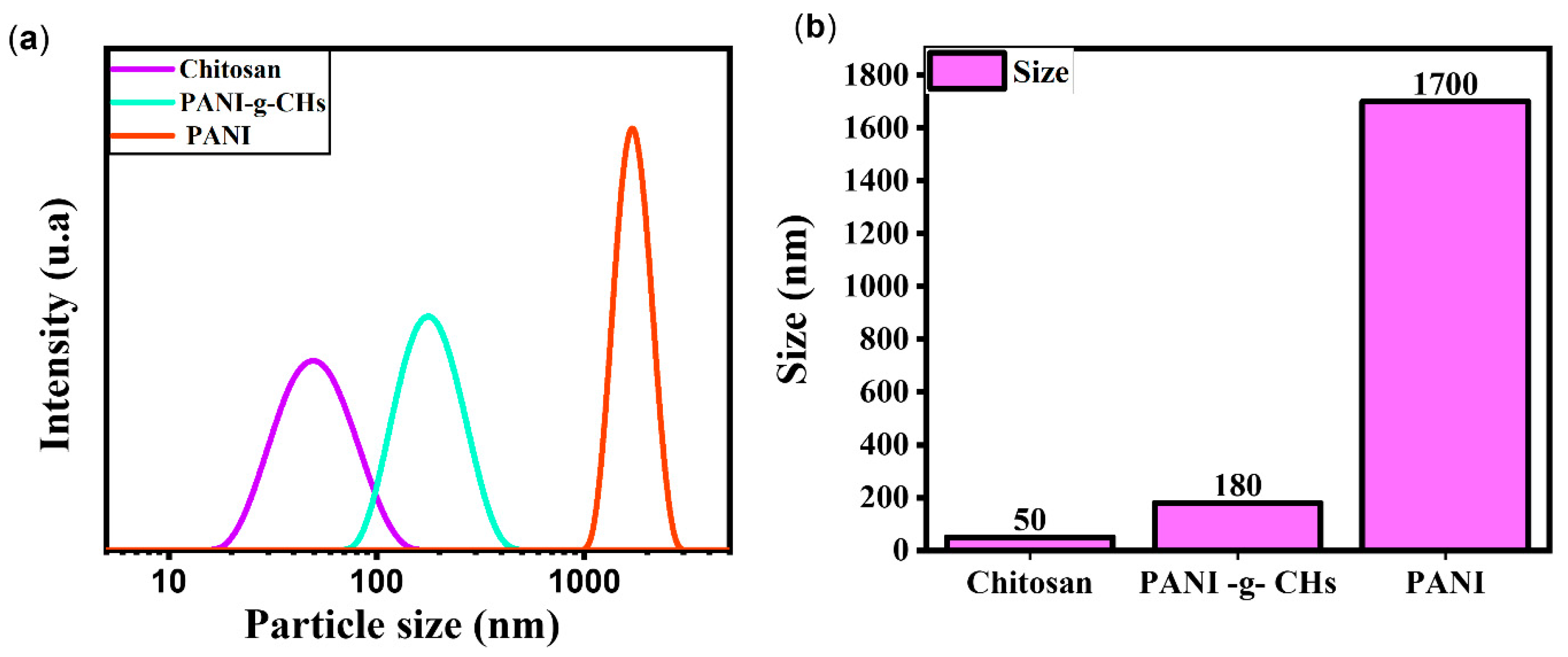
Alcoholic (ethanol) suspensions of PANI, Chs, and PANI-g-Chs at 0.3 g/L were prepared at pH 3. The DLS analysis, reported in Figure 1, showed a uniform distribution [20] for all the nanoparticles (Figure 1a) with a size of 50, 180, and 1700 nm for Chs, PANI-g-Chs, and PANI, respectively. The size reduction from 1700 nm for pristine PANI to 180 nm for PANI-g-Chs indicates that chitosan grafting effectively prevents PANI aggregation due to stabilizing interactions like hydrogen bonding. The uniform distributions suggest better dispersion and smaller particle size.

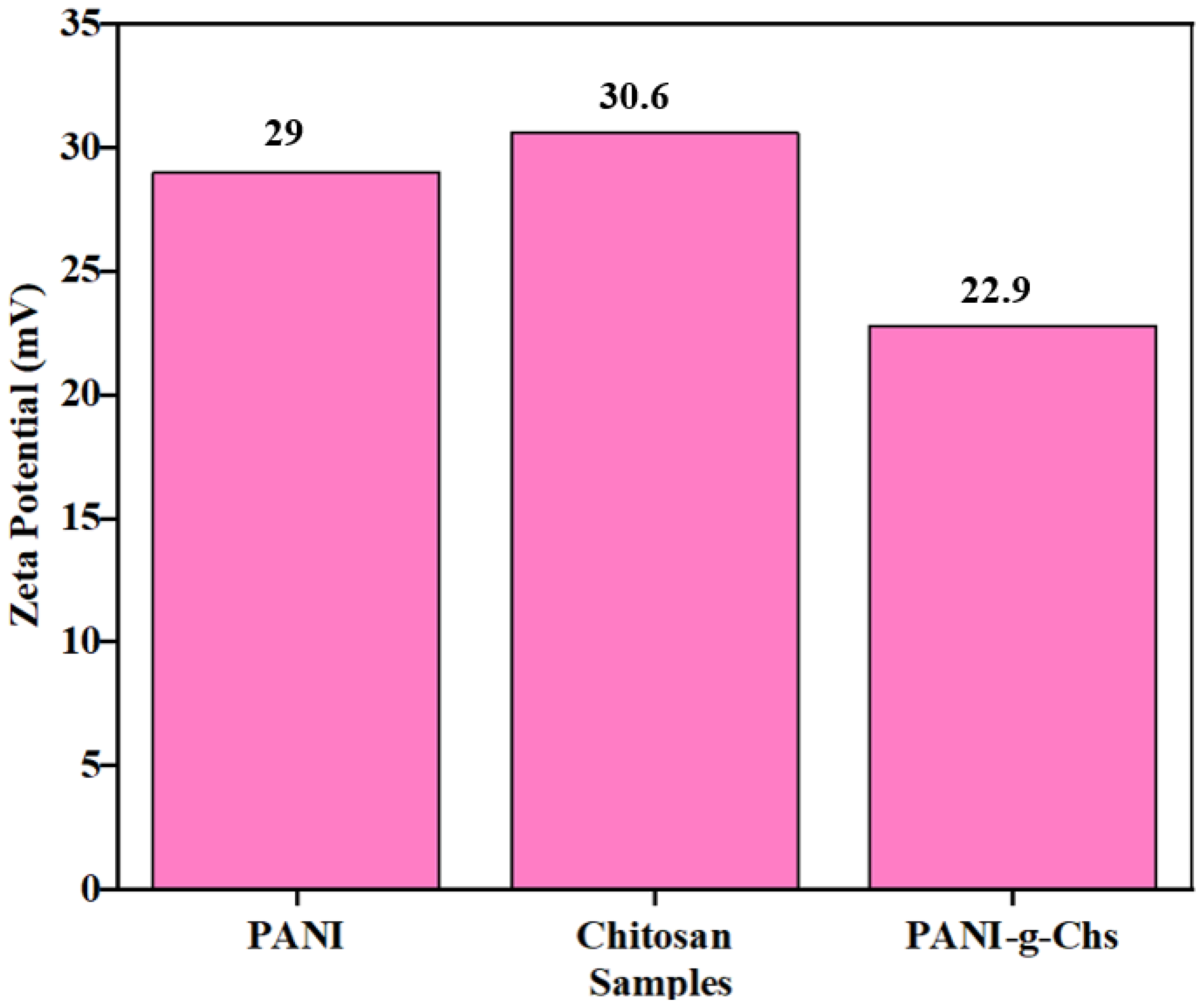
In the evaluation of how stable the systems are when they are charged with electricity, as shown in Figure 2, chitosan and PANI exhibited high positive zeta potential values of +30.6 mV and +29.0 mV, respectively, reflecting their cationic surface nature. The PANI-g chitosan composite showed a slightly lower but still significant positive zeta potential of +22.9 mV. Zeta potential values above +20 mV are generally associated with good colloidal stability due to strong electrostatic repulsion between particles. The moderate decrease observed for PANI-g chitosan can be attributed to partial load screening and redistribution following the grafting process. Nevertheless, the positive surface charge maintained confirms the efficient electrostatic stabilization of the hybrid suspension, which is favorable to the stability of the dispersion.

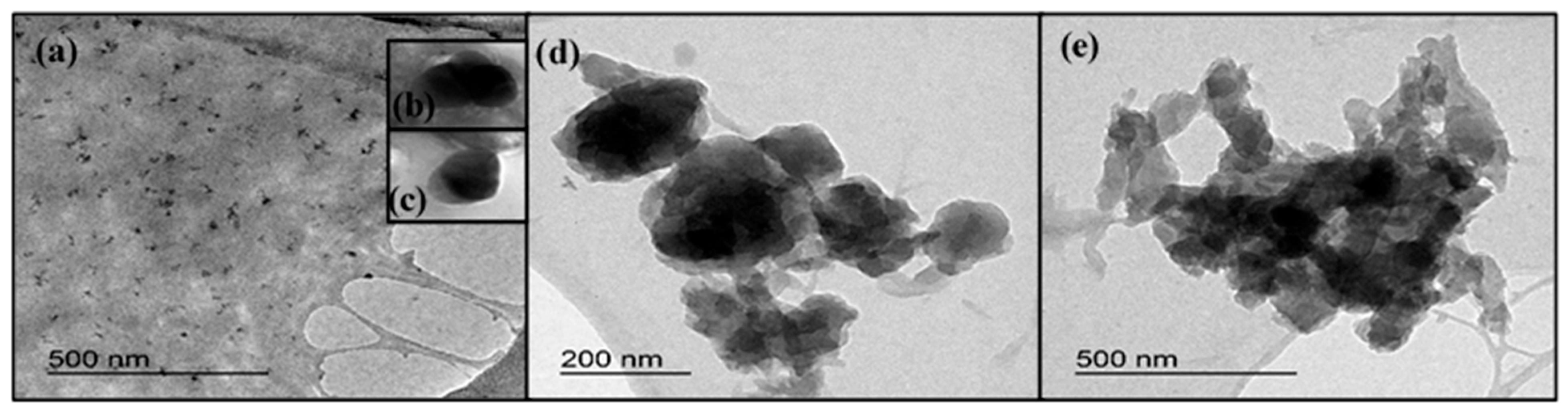
TEM was employed to investigate the morphological characteristics of Chs, PANI, and PANI-g-Chs. As shown in Figure 3a, Chs exhibits a predominantly spherical morphology with uniform distribution across the TEM grid. The particle sizes range from approximately 30 to 100 nm, with an estimated average size of 50 nm. This nanoscale dimension is consistent with previous reports on techniques used for chitosan nanoparticle synthesis [21]. The high-magnification images (inset Figure 3b,c) clearly confirm the spherical shape of the particles. Furthermore, these results are in good agreement with the Chs hydrodynamic diameter measured by DLS. This concordance between the TEM and DLS results confirms both the nanoscale size and the monodispersity of the prepared nanoparticles. The good dispersion and minimal aggregation observed in the TEM images are attributed to the electrostatic stabilization provided by the protonation of amino groups in chitosan under acidic conditions [22], which induces repulsive forces.

The TEM image of PANI-g-Chs (Figure 3d) clearly confirms the successful grafting of polyaniline onto chitosan nanoparticles. The image reveals dense, dark regions corresponding to PANI chains surrounding lighter, spherical cores attributed to the Chs [16]. This core–shell-like morphology suggests that the chitosan nanoparticles retain their spherical shape, typically under 200 nm in diameter, and are partially or entirely encapsulated within the PANI structure. This structural organization indicates strong interaction and effective integration between PANI and Chs, likely through chemical bonding or intermolecular interactions such as hydrogen bonding or electrostatic attraction. The higher electron density of PANI, which appears darker in the image, supports the presence of a conductive shell surrounding the chitosan core. Moreover, the formation of this nanocomposite significantly enhances the dispersion of PANI in the matrix when fabricating biocomposites.

The TEM image of PANI (Figure 3e) reveals an aggregated and irregular morphology, which is characteristic of PANI synthesized via chemical oxidative polymerization. The observed particles form a dense and entangled network, lacking uniform shape and size, with a strong tendency toward aggregation. This behavior is mainly attributed to the π–π interactions between PANI chains, their intrinsic rigidity, and low solubility. The absence of a well-defined nanometric morphology may hinder the homogeneous dispersion of PANI within a polymer matrix, potentially compromising the mechanical and electrical performance of PANI-based composites.

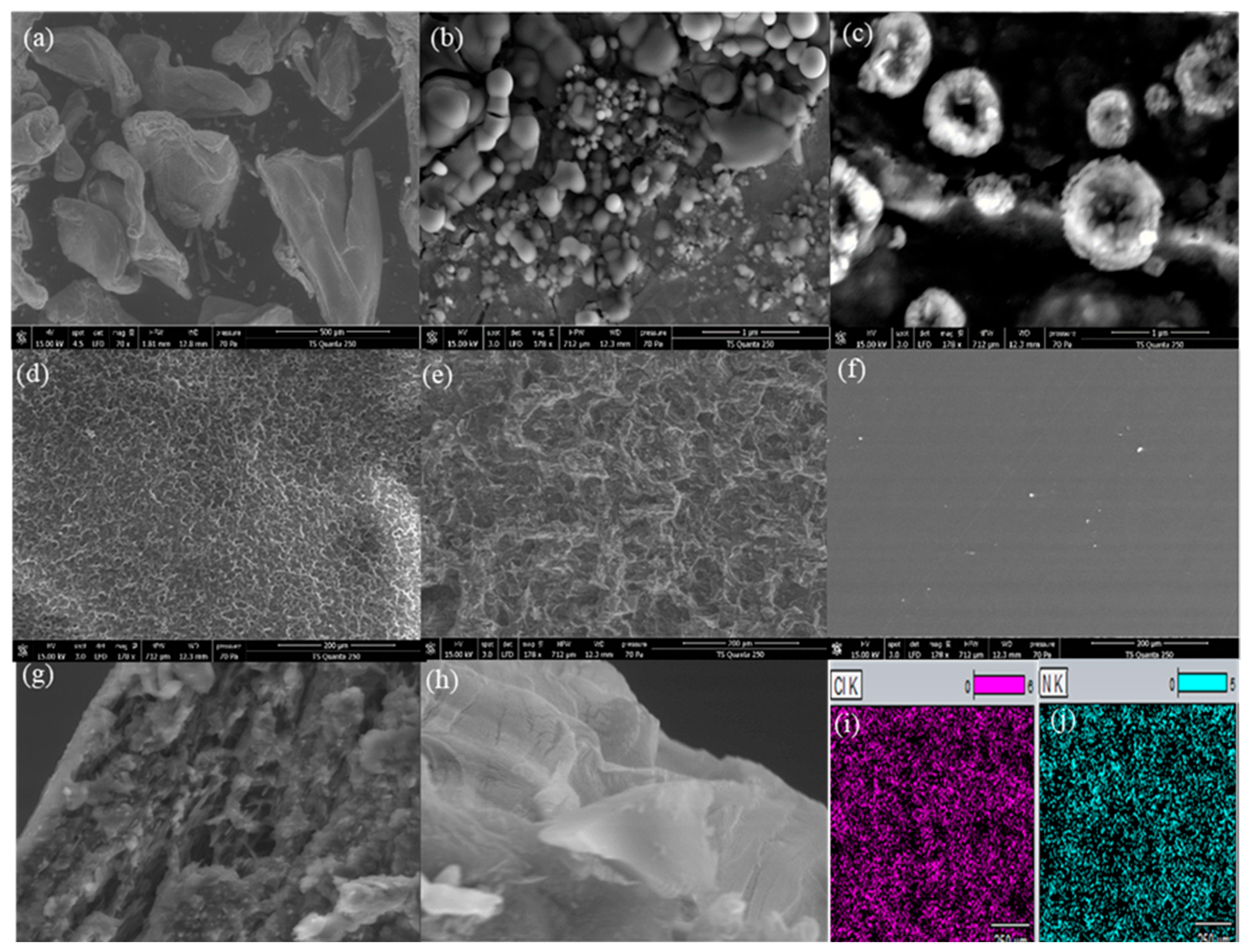
SEM images of commercial chitosan, Chs, PANI-g-Chs, Vinavil film, and Vi-PANI are reported in Figure 4.

Commercial chitosan (Figure 4a) exhibits a typical lamellar morphology, characterized by large, flat, and smooth particles of irregular shape [23]. These sheet-like structures present extensive surfaces with sharp edges, reflecting the crystalline nature of the native biopolymer and its tendency to form ordered stacks. Upon conversion to chitosan nanoparticles (Figure 4b), a significant structural transformation occurs. The SEM images reveal a heterogeneous population of spherical and sub-spherical particles with a broad size distribution, ranging from approximately 50 to 400 nm. The nanoparticles exhibit rough surfaces and a tendency to aggregate, with some particles showing slight deformations. This morphology suggests a formation process driven by controlled crosslinking and precipitation, converting the initial lamellar structure into discrete particulate entities. The PANI-g-Chs composite, Figure 4c, presents spherical, uniform, and well-dispersed particles with a core–shell architecture. These particles display excellent monodispersity and homogeneous diameters as well as a rough, aggregated and clustered morphology. Subtle contrast variations indicate a bilayer structure: a lighter chitosan core surrounded by a denser, more contrasted polyaniline shell [24]. This suggests that the chitosan nanoparticles preserve their integrity while being uniformly encapsulated by grafted PANI. Vinavil film, Figure 4d, exhibits a relatively smooth and homogeneous surface with minimal surface features, characteristic of neat polymer films [25]. The addition of PANI to the Vinavil matrix, Figure 4e,g, results in a more heterogeneous morphology with visible phase separation and rougher surface texture, indicating limited compatibility between the two polymers and PANI aggregation. The corresponding cross section, Figure 4g, reveals a stratified internal structure with delamination zones and poorly bonded interfaces, confirming the weak adhesion between Vinavil and PANI. The isolated PANI aggregates could form discontinuous conductive islands, hinder the formation of an efficient percolation network, and significantly limit electronic transport through the material. In contrast, Vi-PANI-g-Chs, Figure 4f,h, demonstrates remarkably improved morphology with a smoother, more uniform surface. The cross-sectional view, Figure 4h, reveals a compact, dense, and perfectly integrated structure without significant phase separation. This cohesive internal architecture indicates enhanced compatibility achieved through chitosan-mediated grafting, which acts as a molecular bridge between Vinavil and PANI. The structural morphological improvement could translate into superior mechanical and electrical properties: the homogeneous dispersion and reinforced interfacial adhesion enable not only more efficient stress transfer across the film thickness but also the formation of a continuous and interconnected conductive network.

EDS elemental mapping of Vi-PANI-g-Chs reveals a remarkably homogeneous and dense distribution of nitrogen (N) (Figure 4i) and chlorine (Cl) (Figure 4j) across the surface, confirming the effectiveness of PANI grafting onto chitosan.

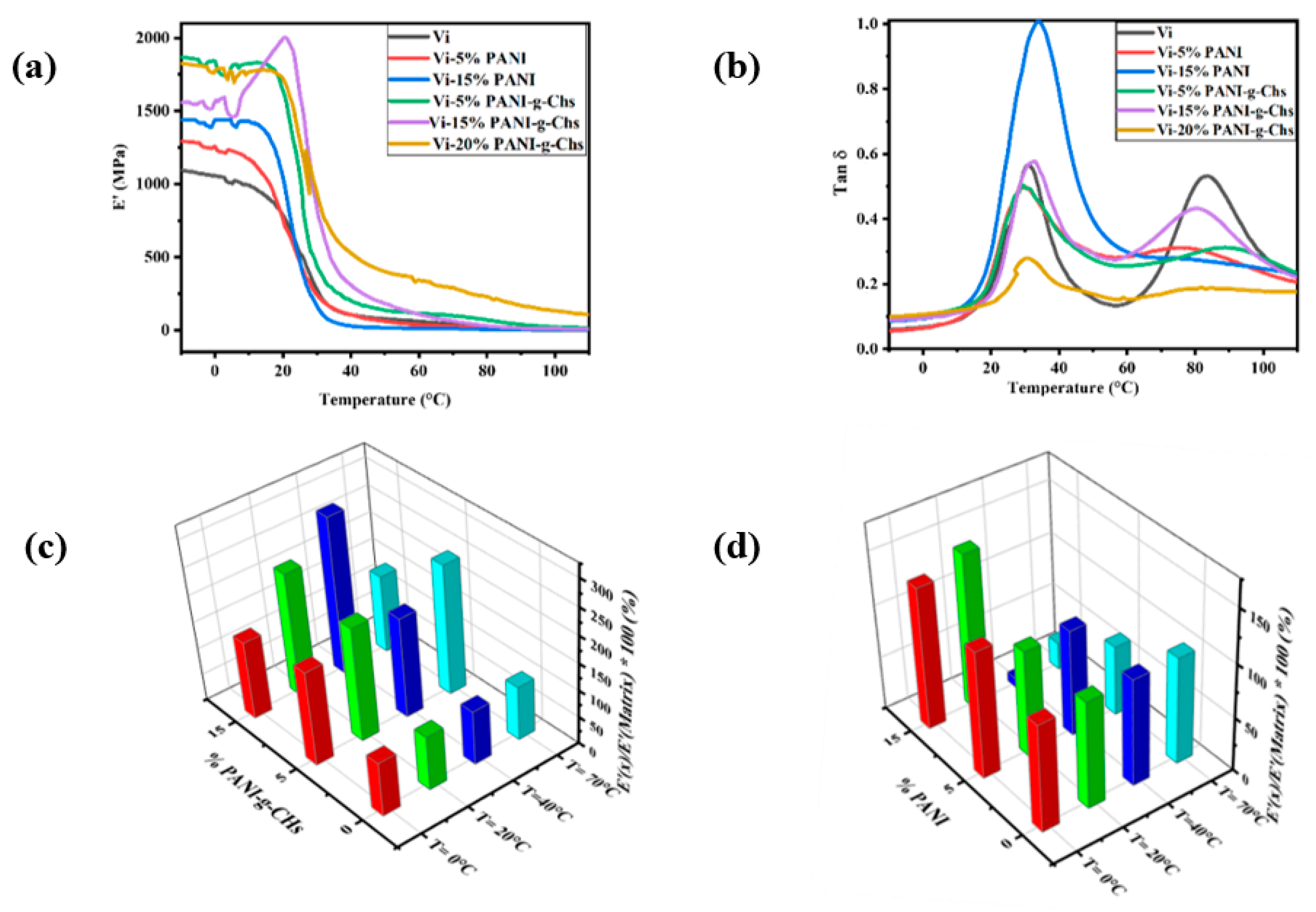
The storage modulus curves, obtained from DMA (Figure 4a), showed that both PANI and PANI-g-Chs enhanced the thermomechanical stability of the Vinavil matrix. At low temperatures, the storage modulus E′ increased with the PANI filler content, indicating improved stiffness. Moreover, the Vi-PANI-g-Chs composites exhibited higher storage modulus values compared to the correlative Vi-PANI, suggesting better interfacial interactions and load transfer efficiency [19]. The tan δ peaks (Figure 4b), representing the glass transition temperature (Tg), showed shifts and intensity changes with increasing filler content, indicating modified molecular mobility and polymer–filler interactions [20], except for the composition at 20% PANI, which shows a visible decrease. This result could be related to filler aggregation at high loadings, which limits effective polymer–filler interactions, as well as to probable heterogeneous distribution or phase separation at high PANI concentrations that may further reduce the overall energy dissipation, leading to a lower tan δ peak.

To investigate the effect of PANI or PANI-g-Chs as filler, the percentage increase in the storage modulus of the nanocomposites was studied (Figure 5c,d) by reporting the histograms of E′(x)/E′(Matrix) × 100, where E′(x) denotes the storage modulus for the nanocomposite, while E′(Matrix) refers to the modulus of Vinavil, at temperatures of 0, 20, 40, and 70 °C. For Vi-PANI (Figure 5c), the maximum enhancement in E′(x)/E′(Matrix)% is obtained at 0 °C and 20 °C with 15 wt% PANI. In contrast, Vi-PANI-g-Chs composites (Figure 5d) demonstrated superior reinforcement for all temperatures investigated, achieving up to 300% improvement at 40 °C with 15 wt% loading. The enhanced performance of PANI-g-Chs composites can be attributed to: (i) improved interfacial adhesion through hydrogen bonding between chitosan and Vinavil [26], (ii) better dispersion of PANI due to chitosan grafting, and (iii) formation of a more effective stress-transfer network.

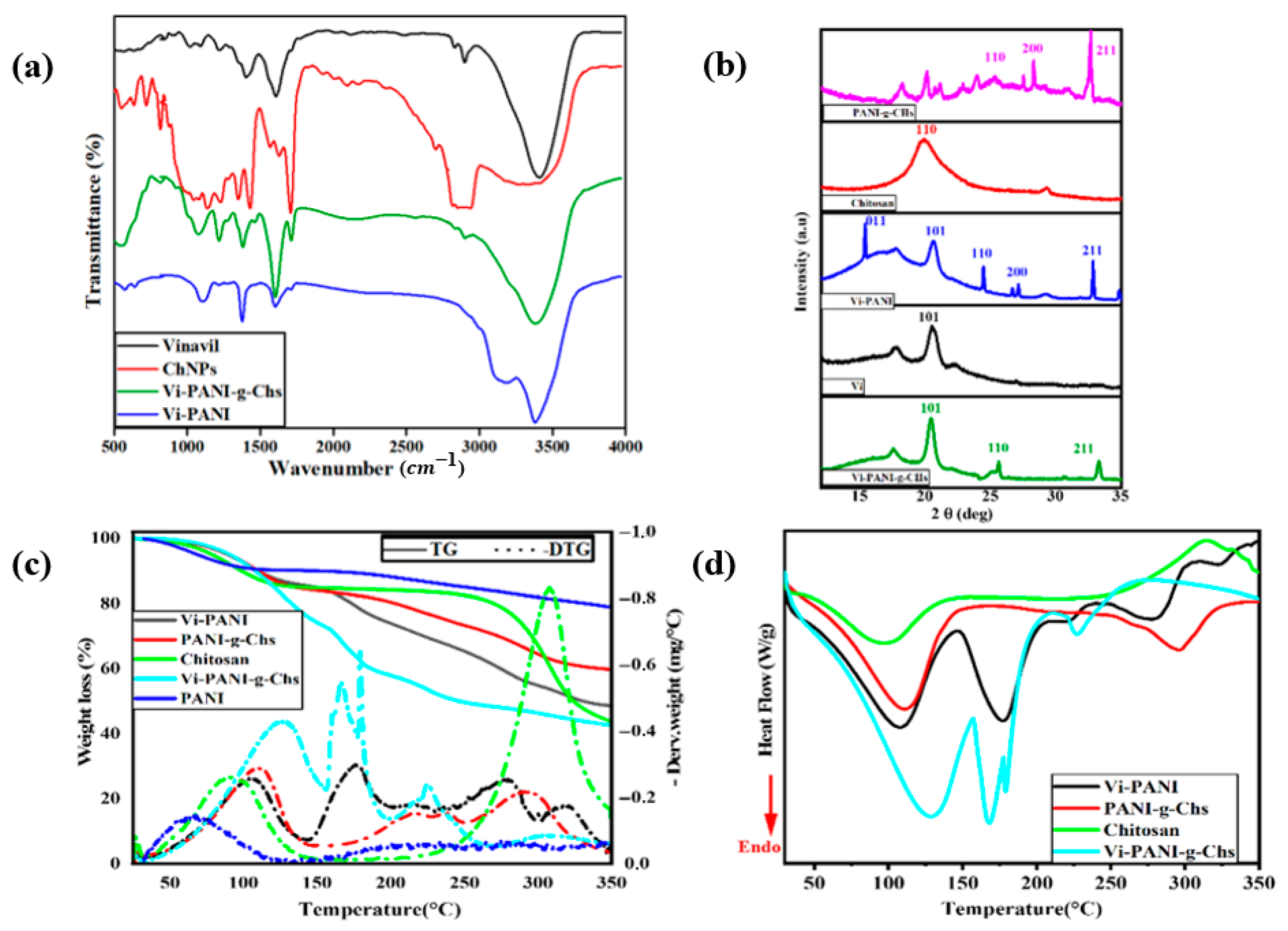
The FTIR spectra of Vinavil, chitosan, Vi-PANI, PANI-g-Chs, and Vi-PANI-g-Chs (Figure 6a) reveal distinctive absorption patterns. The Vinavil matrix spectrum exhibits a broad absorption band centered around 3400 cm⁻¹, corresponding to O-H stretching vibrations of hydroxyl groups, with a characteristic peak around 2900 cm⁻¹ for C-H stretching vibrations of alkyl groups. Additionally, C=O and C-O stretching vibrations from acetate groups appear between 1730 and 1680 cm⁻¹ [27]. For chitosan, the FTIR spectrum shows characteristic bands, including [28,29] a broad absorption band at 3400–3500 cm⁻¹ (3447 cm⁻¹), corresponding to O-H and N-H symmetrical vibrations, CH₂ symmetrical and asymmetrical stretching vibrations centered at 2947 cm⁻¹, distinct peaks in the 1480–1740 cm⁻¹ region, assigned to amide II and I bands, CH₃ symmetrical deformation modes at 1382 and 1417 cm⁻¹, C-O-C glycosidic linkage bands in the fingerprint region below 1200 cm⁻¹, characteristic of saccharides, and C-O stretching vibrations appearing as broad peaks at 1081 and 1122 cm⁻¹.

The FT-IR spectra of Vi-PANI and Vi-PANI-g-Chs show several modifications compared to pristine Vinavil, indicating successful composite formation [30]: a strong absorption around 3200–3400 cm⁻¹, showing hydroxyl (–OH) stretching from the Vinavil matrix and N-H stretching vibrations, and a peak at 1570 cm⁻¹, corresponding to protonated amine groups (NH₃⁺) and quinoid ring stretching typical of polyaniline. The peak at 1408 cm⁻¹ suggests the symmetric stretching vibration of carboxylate groups (COO⁻), which could be attributed to chitosan, while the corresponding asymmetric vibration is masked by overlapping amide II and PANI-related bands. A strong stretching peak at 1100 cm⁻¹ is attributed to the in-plane bending vibration of –CH groups in the benzene ring, confirming the presence of aromatic structures and their role in the polymer’s electronic and mechanical properties [31]. The incorporation of PANI into the Vinavil matrix is confirmed by the characteristic PANI peaks, while the addition of chitosan is validated by the changes in intensity and band shape. These spectral modifications are consistent with the previously reported results from DMA measurements, which show a notable improvement in the mechanical properties of the composite.

The XRD pattern of chitosan exhibits a prominent broad peak at 2θ ≈ 20° (Figure 6b, red curve), which corresponds to the amorphous and semi-crystalline regions of chitosan, attributed to the (110) planes of its polysaccharide backbone stabilized by hydrogen bonding [32]. The XRD pattern of pure Vinavil shows a characteristic broad peak centered at 2θ ≈ 19–20° attributed to the (101) planes (Figure 6b, black curve). The peak of Vinavil at 2θ ≈ 19–20° related to the (101) crystalline planes is evident in the Vi-PANI and Vi-PANI-g-Chs samples, though with varying intensities and slight shifts [33]. The broadness and low intensity of this peak indicate a highly amorphous structure, suggesting enhanced flexibility but reduced mechanical strength, making this VI sample suitable for applications such as flexible coatings or packaging films.

The XRD pattern of PANI-g-Chs exhibits a broad peak at 2θ ≈ 20°, accompanied by smaller peaks at 25° and 30° and a sharp peak at 35° (Figure 6b, magenta curve). The broad peak at 20° results from the overlap of chitosan’s amorphous region (20°) and PANI’s semi-crystalline peak (20°), indicating a predominantly amorphous structure with some residual crystallinity from PANI. The peaks at 2θ ≈ 25°, 30°, and 35° correspond to the (110), (200), and (211) reflections of PANI’s emeraldine salt form, respectively, confirming that PANI retains crystalline order despite grafting [34]. The emeraldine salt structure consists of alternating quinoid and benzenoid rings with nitrogen atoms in both amine and imine forms, providing optimal charge delocalization [35]. The conductive properties are further enhanced by the formation of crystalline domains, as evidenced by XRD peaks at 2θ ≈ 25°, 30°, and 35°, which correspond to the characteristic d-spacings of the emeraldine salt structure [36].

The shift of the broad peak to 2θ ≈ 20° in PANI-g-Chs and the reduced intensity of PANI’s characteristic peaks suggest that grafting disrupts crystallinity, likely due to interactions between PANI chains and chitosan’s functional groups through hydrogen bonding. The sharp peak at 2θ ≈ 35° indicates high orientation in the (211) plane, while the lower intensity of the (110) and (200) peaks suggest a smaller population of crystallites, consistent with structural disorder introduced by chitosan. The XRD pattern for the Vi-PANI blend (Figure 6b, blue curve) reveals multiple peaks, including a small broad peak at 2θ ≈ 16°, a broad peak at 2θ ≈ 19–20°, a smaller broad peak at 2θ ≈ 25°, a sharp peak at 2θ ≈ 29°, and a smaller peak at 2θ ≈ 35°. The peak of Vinavil at 2θ ≈ 19–20° related to the (101) planes is evident in this sample, though with reduced intensity due to blending effects. The peaks at 2θ ≈ 25°, 29°, and 35° align with the (110), (200), and (211) reflections of PANI’s emeraldine salt form, confirming conductivity retention despite blending. The reduced intensity of both Vinavil and PANI peaks, along with the slight shift of PANI’s (200) peak from 2θ ≈ 30° to 2θ ≈ 29°, suggests molecular interactions, such as hydrogen bonding between Vinavil’s hydroxyl groups and PANI’s amine/imine groups, which disrupt the crystalline order of both components [37].

The XRD pattern for the Vi-PANI-g-Chs blend exhibits a broad peak at 2θ ≈ 20° and smaller peaks at 2θ ≈ 25° and 2θ ≈ 35° (Figure 6b, green curve). The peak of Vinavil at 2θ ≈ 20° related to the (101) crystalline planes is evident in this ternary blend, overlapping with contributions from chitosan’s amorphous region and PANI’s (100) plane. This creates a highly amorphous structure due to complex intermolecular interactions. The peaks at 2θ ≈ 25° and 2θ ≈ 35° correspond to the (110) and (211) reflections of PANI’s emeraldine salt form, confirming retention of conductive properties in the composite system.

The predominantly amorphous nature of this composite, combined with PANI’s crystalline regions, indicates multifunctionality, balancing flexibility, biocompatibility, and conductivity, making it suitable for biomedical applications such as flexible biosensors, tissue engineering scaffolds, or flexible conductive films.

Thermogravimetric analysis (TGA), derivative thermogravimetry (DTG), and differential scanning calorimetry (DSC) were performed to evaluate the thermal stability and structural transitions of the synthesized materials (Figure 6c,d).

ATG and DTG curves reveal distinct multi-step decomposition profiles. The degradation onset temperature (T_onset), defined as the temperature at 5% mass loss after moisture removal, is the key parameter for the practical assessment of thermal stability.

Pure PANI exhibits remarkable thermal stability, retaining approximately 85% of its mass up to 350 °C. It exhibits the highest intrinsic stability, with T_onset > 300 °C. Main degradation occurs between 400 and 600 °C, attributed to the cleavage of the conjugated aromatic structure, followed by a slow burning of the nitrogen-rich carbonaceous residue above 600 °C [6,7]. Commercial chitosan displays thermal behavior characteristic of polysaccharides. TGA reveals a three-stage degradation process: (i) dehydration (<120 °C), (ii) depolymerization and degradation of the saccharide units (T_onset = 250 °C, major peak at 300 °C), and (iii) slow oxidative degradation of the carbonaceous residue (>400 °C) [8,9].

The PANI-g-Chs graft copolymer manifests distinct thermal properties, confirming successful grafting. Grafting modifies the profiles, with two main steps: T_max1 (230–250 °C), related to chitosan graft cleavage, and T_max2 (300 °C), corresponding to PANI skeleton fragmentation. The global T_onset drops to 220 °C, indicating earlier degradation than for pure PANI [38].

The Vi-PANI blend displays reduced crystallinity compared to its pure constituents, as confirmed by TGA, with degradation in four phases: (i) evaporation of water and solvents (<150 °C), (ii) decomposition of Vinavil chains and deacetylation (180 °C), (iii) scission of the Vinavil skeleton and initial degradation of PANI (275 °C), and (iv) final burning of the residue (325 °C). The onset of degradation (T_onset) occurs at 200°. These characteristics suggest strong molecular interactions between Vinavil and PANI [14].

The Vi-PANI-g-Chs ternary blend exhibits the most complex thermal behavior, characterized by the lowest thermal stability among the studied materials, T_onset 150–180 °C. DTG reveals a succession of closely spaced peaks, reflecting an interactive and catalytic mechanism: (i) dehydration and deacetylation (<150 °C), (ii) simultaneous degradation of the Vinavil chains and chitosan grafts (150–200 °C), (iii) fragmentation of PANI (200–250 °C), and (iv) oxidation of carbon residues (300–350 °C). These interactions lower the energy threshold for decomposition compared to isolated components [39,40].

DSC thermograms complement the ATG:

Bounded water evaporation: The wide endothermal peak between 80 and 120 °C for samples containing chitosan and/or Vinavil corresponds to the first mass loss in ATG.

PANI-g-Chs: The peak at 300 °C corresponds to the DTG peak, confirming that heat flux is dominated by chemical reactions and not reversible physical transitions.

Vi-PANI-g-Chs: A series of endothermic events occurs, distributed between 150 and 300 °C, completely masking the glass transition (Tg) due to interactive and early degradations.

In summary, the thermal analysis reveals that while grafting and blending successfully modify polymer properties, they generally result in decreased thermal stability compared to pure PANI. The low thermal stability of the ternary mixture (T_onset 150 °C), combined with the complexity of its degradation mechanisms, constitutes a major obstacle for its use in high-power flexible electronic devices. To prevent the initiation of decomposition, emission of byproducts and alteration in electrical or mechanical properties, the operating temperature should be strictly limited, ideally below 120–140 °C.

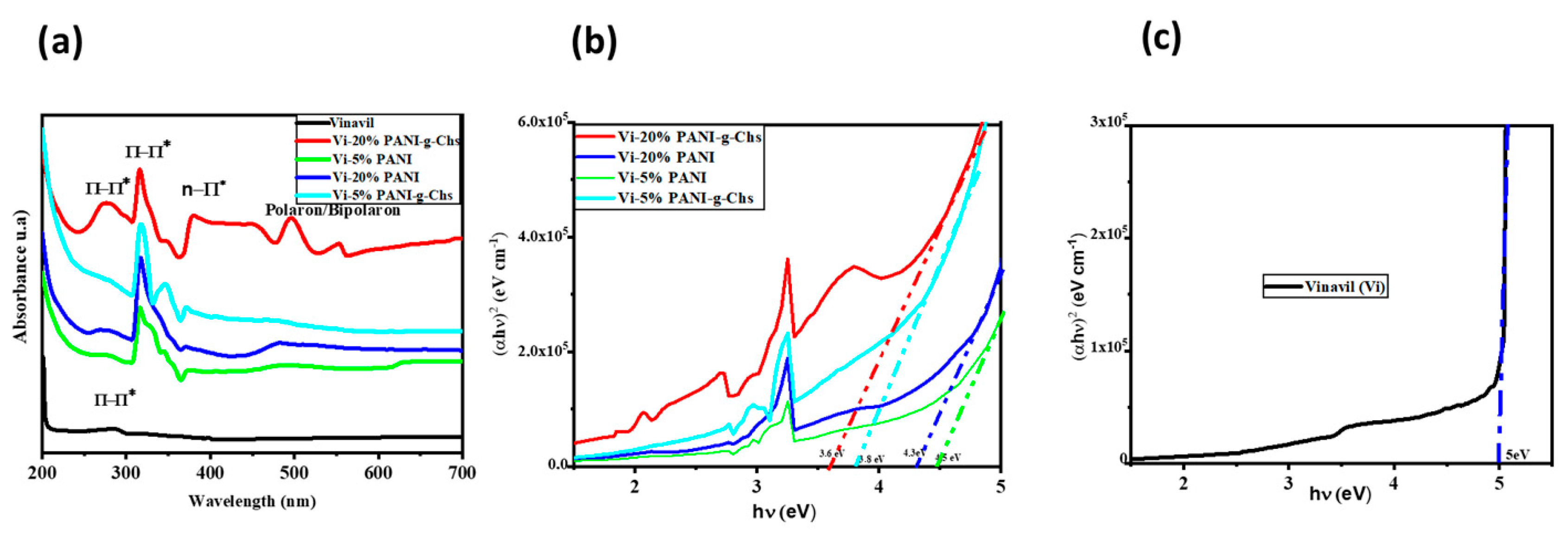
The UV-vis spectra of Vinavil, PANI, and PANI-g-Chs are reported in Figure 7. The Vinavil matrix shows a peak at 280 nm, corresponding to the π-π* transition, characteristic of the residual acetate groups [41,42]. For Vi-PANI blends, the spectrum reveals distinct peaks at 320–332 nm attributed to π-π* transitions within the phenyl and quinoid rings of PANI. The intensity of these peaks progressively increases with the PANI concentration, indicating enhanced conjugation and a higher density of aromatic structures in the polymer matrix. At a higher PANI content, polaron/bipolaron transitions emerge at 400–440 nm, characteristic of PANI’s conducting state. This spectral evolution demonstrates that increasing the PANI concentration enhances the intensity of the characteristic absorption bands and promotes the formation of the conducting emeraldine salt form. The Vi-20% PANI sample shows more pronounced polaron/bipolaron bands compared to Vi-5% PANI, where these transitions remain relatively weak, indicating improved charge carrier generation with higher PANI loading.

Remarkably, the Vi-PANI-g-Chs samples display significantly enhanced conducting characteristics compared to simple Vi-PANI blends. The π-π* transition peaks at 320–332 nm are not only preserved but appear more intense and well-defined, suggesting improved molecular organization and stronger electronic interactions due to PANI–chitosan grafting. Most notably, the polaron/bipolaron transitions at 400–440 nm are considerably more pronounced in Vi-PANI-g-Chs samples, even at lower PANI concentrations. This enhancement indicates that grafting PANI onto chitosan promotes a more stable conducting state by facilitating better doping efficiency and charge carrier mobility. The Vi-20% PANI-g-Chs sample exhibits the strongest and broadest polaron/bipolaron absorption band among all samples, demonstrating superior conductivity arising from the synergistic interactions between PANI’s conjugated backbone and chitosan’s functional groups. With the presence of PANI grafted onto chitosan (Vi-PANI-g-Chs), several distinct peaks are observable, highlighting the complex interactions between the composite components (Figure 7a).

The bandgap energy (Eg) was calculated using the Tauc relation [43]:

αhυ = A(hυ − Eg)ⁿ

(1)

where α is the absorption coefficient, hν is the photon energy (1240/λ), A is a constant, and E_g is the bandgap energy. The Tauc plot of (αhν)² versus hν (Figure 7b,c) was used to estimate E_g by extrapolating the linear portion of each curve to the energy axis. The estimated bandgaps are reported in

Table 3. Bandgap energy and number of carbon atoms per cluster of Vi-PANI and Vi-PANI-g-Chs with different w%.

Samples	Eg (eV)	No. of Conjugated Carbon Atoms (N)	No. of Carbon Atoms per Cluster (M)
Vinavil	5.0	-	47
Vi-5%PANI	4.5	4	58
Vi-20%PANI	4.3	4	64
Vi-5%PANI-g-Chs	3.8	5	82
Vi-20%PANI-g-Chs	3.6	5	91

.

The decrease in Eg from 5.0 eV for Vinavil to 4.3 eV with 20% PANI in Vin-20%PANI confirms that a higher PANI content enhances the conductivity of the matrix.

The observed decrease in the Eg of Vin-20%PANI-g-Chs (3.6 eV) compared to Vi-20%PANI (4.3 eV) suggests that grafting polyaniline onto chitosan significantly modifies the electronic structure of the conducting polymer, leading to improved electrical conductivity. This phenomenon can be attributed to different causes: (i) chitosan’s amine groups (–NH₂) may protonate PANI imine sites (=N–), increasing polaron density and delocalization [44]; (ii) grafting can enhance PANI dispersion in the Vinavil matrix, reducing charge trapping at agglomerates and hydrogen bonding between PVA’s –OH; and (iii) PANI-g-Ch_S –NH₂ groups may create percolation pathways for charge transport [31].

Two key parameters can be calculated from optical bandgap measurements using established theoretical models: N (number of conjugated carbon atoms) and M (number of carbon atoms per cluster) (Table 3). The number of carbon atoms (N) refers to the number of carbon atoms involved in the conjugation along a linear polymer chain. It influences the electronic and optical properties of the polymer. It was calculated using the equation given by Robertson and O’Reilly [45]:

$$\mathrm{N}={\displaystyle \frac{2\mathsf{\beta }\mathsf{\pi }}{\mathrm{E}\mathrm{g}}}$$

(2)

where β is taken to be −2.9 eV, as it is associated with π-π* optical transitions in C=C linkages, and Eg is the lower value of the bandgap.

The number of carbon atoms per cluster (M) refers to the size of an aggregate or group of molecules in a material. In polymers, this could be related to the size of the clusters of polymer chains that interact with each other and was calculated using Equation [45]:

$$\mathrm{M}={\displaystyle \frac{{34.3}^2}{{{\mathrm{E}}_{\mathrm{g}}}^2}}$$

(3)

where E_g is the lower energy bandgap.

The increase in N from 0 (Vinavil) to 4 (Vi-5%PANI and Vi-20%PANI) and to 5 (Vi-5%PANI-g-Chs and Vi-20%PANI-g-Chs) reflects the progressive introduction of conjugation by PANI and its extension by chitosan grafting, while M increases from 47 to 91, indicating larger conjugated clusters. The unchanged values of N observed for Vi-5%PANI and Vi-20%PANI suggest poor dispersion in the absence of chitosan, limiting conjugation. This is in perfect agreement with the bandgap decrease from 5 eV (Vinavil) to 3.6 eV (Vi-20%PANI-g-Chs) and the increased conductivity observed.

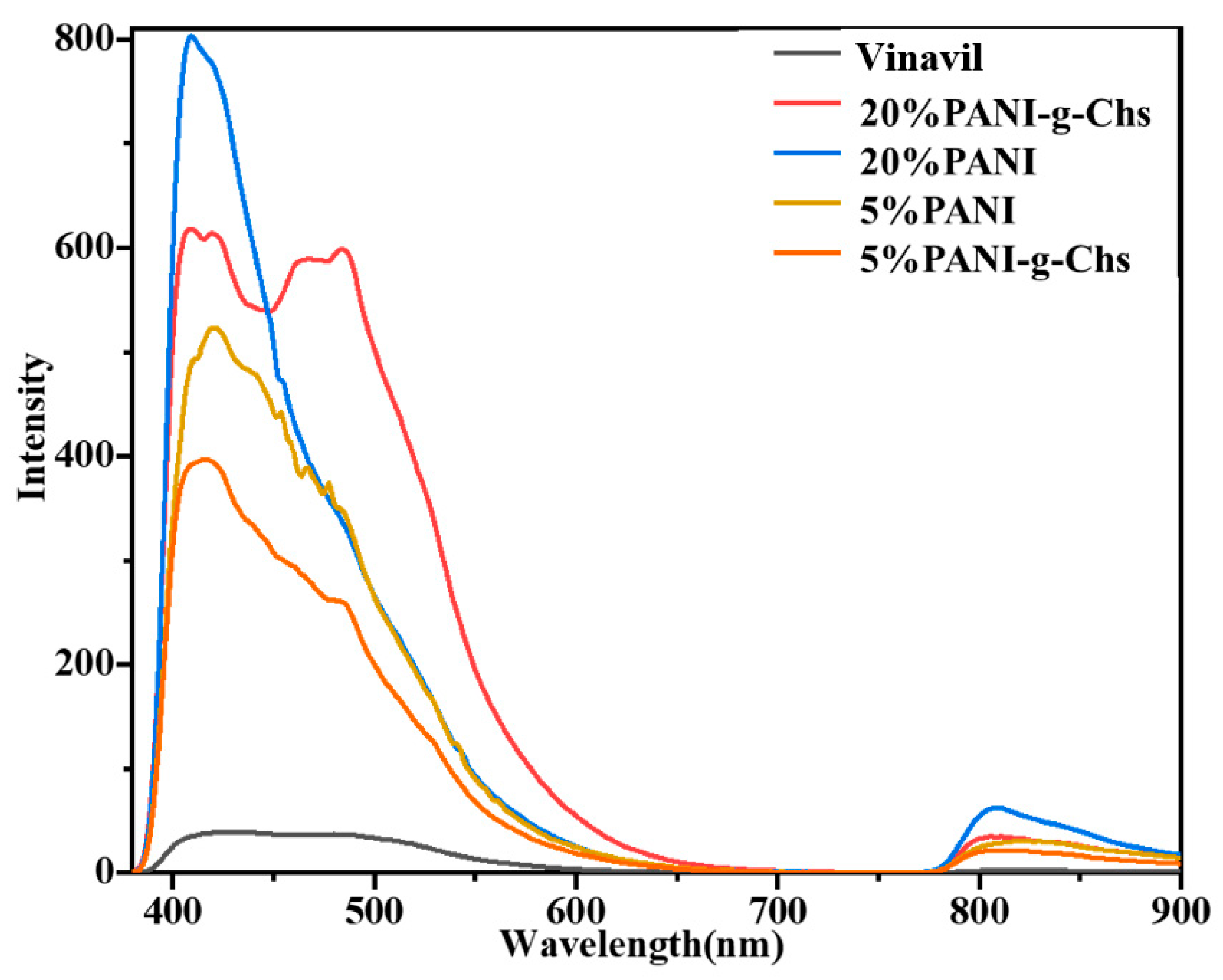
Figure 8 shows the photoluminescence (PL) spectra of Vinavil, Vi-5%PANI, Vi-20%PANI, Vi-5%PANI-g-Chs and Vi-20%PANI-g-Chs measured at room temperature at an excitation wavelength in the UV region (350 nm). The presence of PANI gives two main photoluminescence emission peaks: an intense emission peak in the visible region at 410–450 nm and a small secondary peak around 800–850 nm. The first emission at 410–450 nm is attributed to the π–π* transition of the benzenoid units of polyaniline, an observation consistent with the literature [37,38]. The small secondary peak at 800–850 nm is due to the electronic transitions of the polaronic and bipolar states of PANI. These states are induced by the protonation of imine nitrogen atoms, forming polarons/bipolarons. These localized states create intermediate energy levels in the bandgap, between the valence band (BV) and the conduction band (BC), resulting in lower energy emission (1.46–1.55 eV) relative to the main π–π* transition [46]. It is important to note that the emission in the 410–450 nm range may include a contribution from scattering effects when UV light is used for excitation. However, its dependency on PANI content and the existence of NIR emission bands support its assignment to PANI-related electronic transitions. The intensity and the maximum position of these emission peaks vary considerably according to the concentration of PANI. The incorporation PANI-g-Chs widens the emission profile, with a notable shoulder around 500 nm, suggesting a modification of the electronic structure of PANI due to grafting, probably associated with an increase in conjugation and a decrease in the bandgap, in agreement with the results previously discussed. It is possible that the quinonoid units present in the PANI partially attenuate the PL emission by promoting the dissipation of intra-chain energy, which explains the decrease in intensity observed for samples grafted with chitosan [46].

To better investigate the effect of the addition of PANI and PANI-g-Chs, the electrical conductivities of Vinavil, Vi-5%PANI, Vi-10%PANI, Vi-15%PANI, Vi-20%PANI, Vi-25%PANI, Vi-5%PANI-g-Chs, Vi-10%PANI-g-Chs, Vi-15%PANI-g-Chs, Vi-20%PANI-g-Chs, and Vi-25%PANI-g-Chs (1.0 cm² samples with a thickness of 1.0 mm) were investigated with four-point probe measurements, complemented by Hall effect analysis (Figure 8,

Table 4. Four-probe measurement results.

Samples	%	Conductivity (S/m)	Resistivity (Ohm m)	Sheet Resistance (Ω/sq)
Vi-PANI	15	0.49	2.07	2065.17
	25	14.02	0.07	71.31
Vi-PANI-g-Chs	15	3.43	0.29	292.02
	25	77.79	0.01	12.85

and

Table 5. Hall effect measurements.

Samples	Test N°	Carrier Density Variations (cm−3)	Resistivity (Ohm·m)	Conductivity (S/cm)	Mobility (cm2/V·s)	Avg. Hall
Vi-25%PANI-g-Chs	1	−6.5403 1015	0.82084	1.2183	1162.7	−954.42
	2	1.4344 1015	5.575	0.17937	780.58	4351.8
Vi-15%PANI-g-Chs	1	1.2928 1013	35.494	0.02817	136.04	48,285
	2	−3.7386 1014	41.898	0.02387	398.51	−16,697
Vi-25%PANI	1	−4.9078 1015	15.802	0.06328	80.486	−1271.9
	2	6.1231 1015	17.09	0.05851	59.653	1019.4
Vi-15%PANI	1	−1.3581 1015	716.95	0.00139	6.107	−4596.1
	2	7.3539 1015	1924	5.1975 × 10−4	0.4411	848.83

).

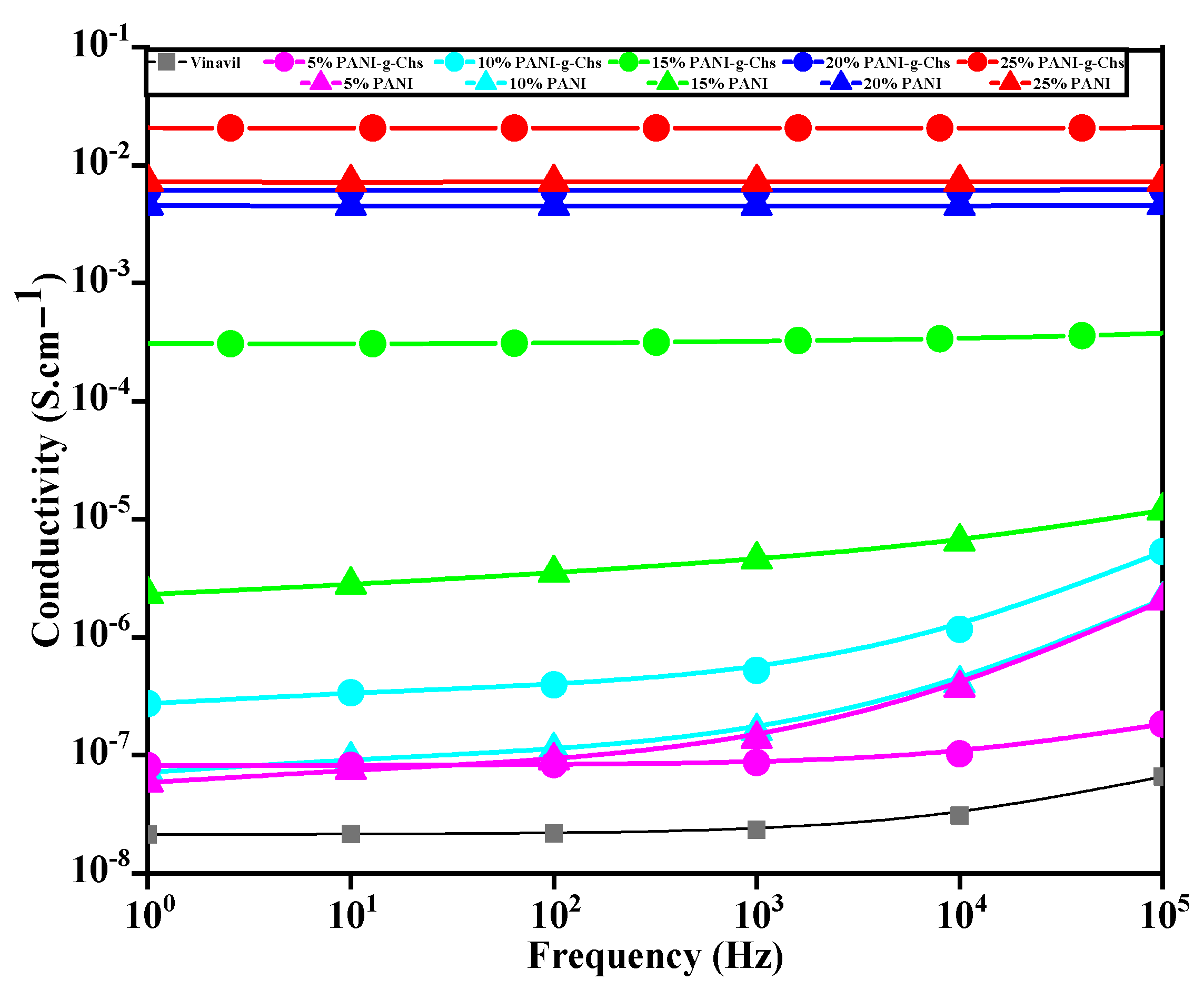
As observed in Figure 9, the addition of PANI or PANI-g-Chs gives a clear enhancement in the electrical conductivity. This increase depends on the amount of additive used. The presence of PANI-g-Chs significantly enhanced the electrical performance compared to PANI at equivalent concentrations. The highest conductivity of 5.10⁻² S·cm⁻¹ was observed for the Vi-25%PANI-g-Chs film with respect to Vinavil (conductivity of c.a. 10⁻⁸ S·cm⁻¹) with an improvement of about six orders of magnitude. Again, the better dispersion of the conductive phase within the Vinavil matrix, the reduced aggregation, and the formation of a more continuous conductive network could promote efficient charge transport.

Moreover, highly conductive samples (e.g., Vi-25%PANI-g-Chs, Figure 9) exhibited a constant conductivity for the entire frequency range, characteristic of metallic or semi-metallic conduction behavior. In contrast, samples with lower conduction (Vi-5%PANI) showed a pronounced frequency dependence, characteristic of a hopping conduction mechanism between localized states.

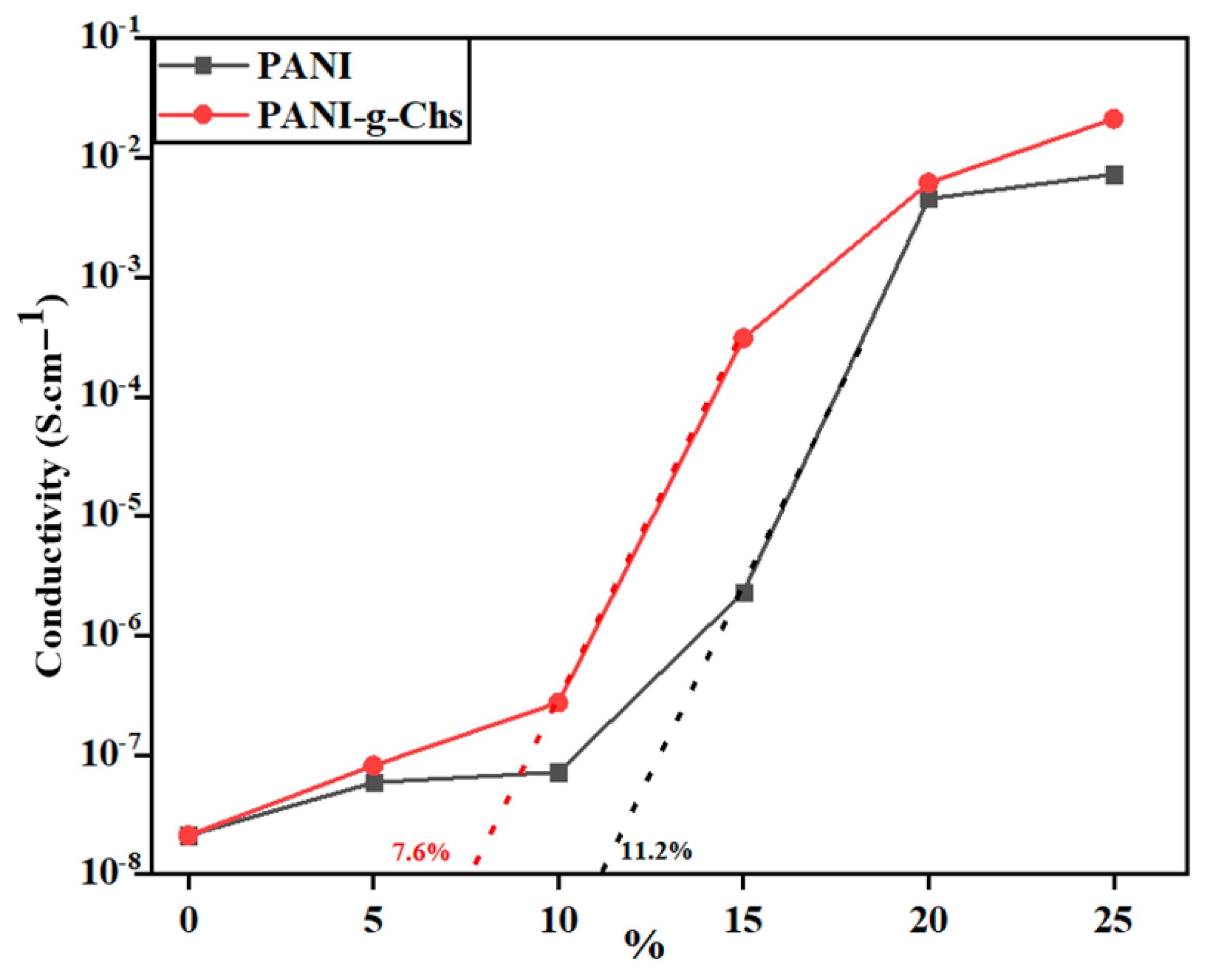
A distinct percolation threshold was observed between 5% and 15% loading for both types of conductive fillers. Specifically, the PANI-g chitosan composite reached its percolation threshold at 7.6% (Figure 10), while pure PANI required a higher loading of 11.2%, indicating that grafting with chitosan promotes more efficient network formation. Beyond 15–20%, the conductivity increase began to plateau, indicating a saturation effect in the conductive network.

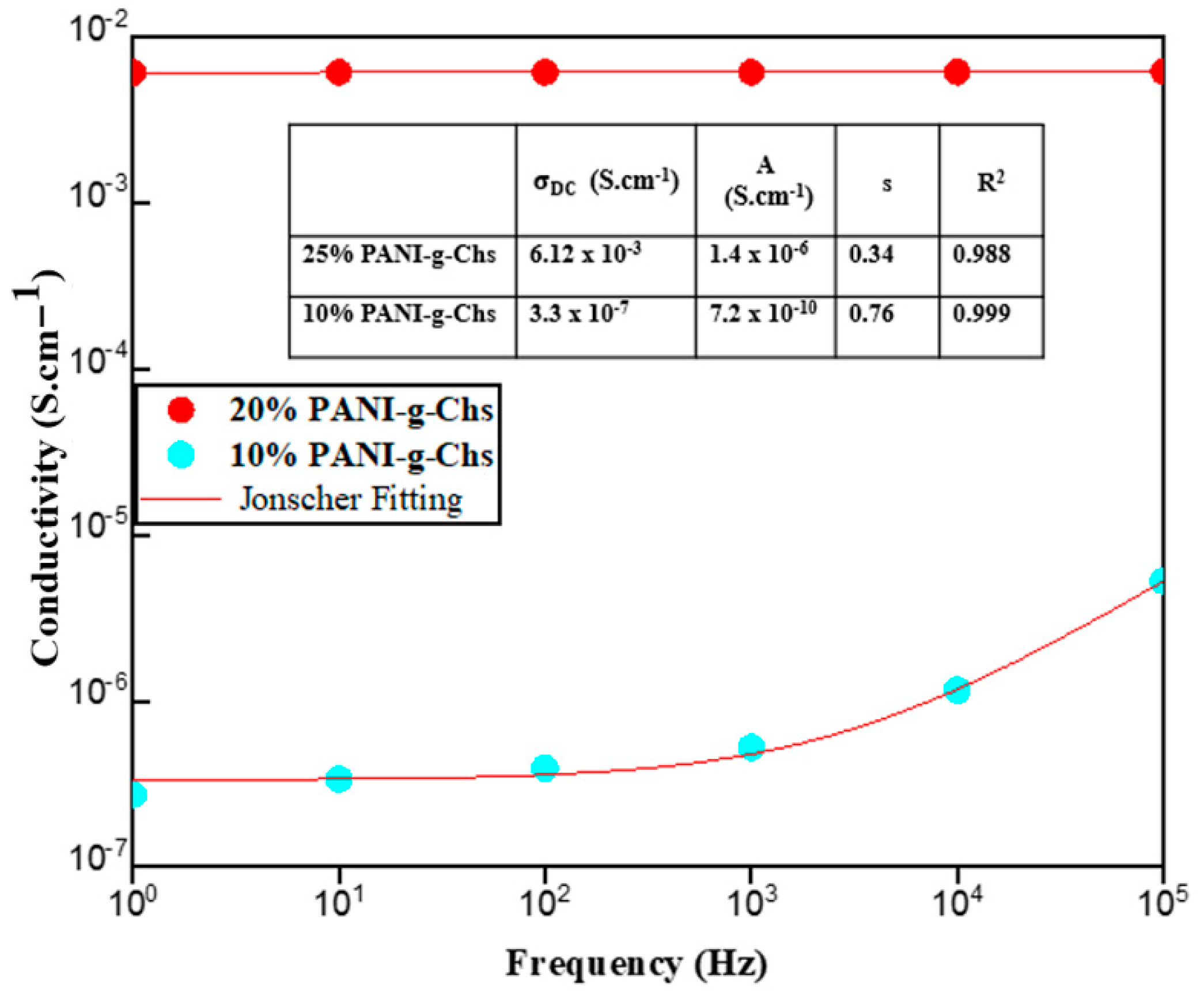
Figure 11 illustrates the frequency dependence of AC conductivity for the 20% and 10% PANI-g-Chs composites fitted using the Jonscher power law:

$$\sigma \left(\omega \right)={\sigma }_{DC}+\mathrm{A}{\omega }^s$$

(4)

In the low-frequency region, the 20% PANI-g-Chs composite exhibits almost frequency-independent conductivity, indicating that the electrical response is dominated by DC conductivity. This behavior, associated with a low Jonscher exponent (s = 0.34), suggests long-range charge transport through well-established percolation pathways.

Conversely, the 10% PANI-g-Chs composite shows a clear increase in conductivity with frequency, particularly beyond the low-frequency region. The higher exponent (s = 0.76) reflects a strong frequency dependence, characteristic of localized charge carrier hopping between defect or localized states in a disordered polymer network.

Overall, the Jonscher analysis demonstrates a transition from DC-dominated conduction at a higher PANI-g-Chs loading to AC-dominated, hopping-controlled conduction at a lower loading. This tunable electrical behavior highlights the role of filler concentration in controlling charge transport mechanisms in PANI-g-Chs composites.

Table 4 reports the four-probe measurement results related to Vi-PANI (15% and 25%) and Vi-PANI-g-CHs (15% and 25%).

As observed in Table 4, the incorporation of PANI-g-Chs gives superior electrical performance compared to PANI, corresponding to a 7- or 5-fold increase. The resistivity values showed an inverse correlation with the conductivity measurements. The sheet resistance values ranged from 2065.17 Ω/sq for Vi-15%PANI to 12.85 Ω/sq for Vi-25%PANI-g-Chs, leading to a transition from insulating to semiconducting behavior. The maximum conductivity obtained for Vi-25%PANI-g-Chs (77.79 S/m; 0.778 S/cm) approaches the range typically associated with high-performance semiconducting polymer systems [47] and exceeds the requirements for antistatic applications by several orders of magnitude.

Complementary Hall effect measurements provided crucial insights into the charge transport mechanism, revealing the dominant charge carrier type and mobility values that support the conductivity enhancement observed through chitosan grafting, with detailed results summarized in Table 5.

Under an applied magnetic field of 0.554 T, with an initial current of 1.0 µA and a film thickness of 1.0 mm, Vi-PANI-g-Chs demonstrated a remarkable improvement in electronic transport properties compared to Vi-PANI. Vi-25%PANI-g-Chs exhibited a maximum conductivity of 1.22 S/cm with an exceptional mobility of 1163 cm²/V·s, representing a 20-fold improvement in conductivity and an enhancement in mobility of more than an order of magnitude compared to Vi-25%PANII (σ = 0.063 S/cm, µ = 80 cm²/V·s). This significant enhancement in charge carrier mobility agrees with the more ordered conductive pathways and reduced charge scattering at interfaces observed with PANI grafted onto chitosan. The alternation between positive and negative values observed (Avg Hall, Table 3) indicates the coexistence of majority and minority carriers, typical of complex conducting polymer systems. The positive carriers observed correspond primarily to polarons and bipolarons formed during the polyaniline doping process; these positively charged quasi-particles are responsible for conduction in the conducting segments of the conjugated polymer. The conductivity enhancement from 0.063 to 1.22 S/cm demonstrates the superior charge transport efficiency due to PANI grafted onto chitosan, while the dramatic mobility increase from 80 to 1163 cm²/V·s indicates reduced charge scattering and improved charge delocalization along the polymer backbone.

The carrier density variations (ranging from 10¹³ to 10¹⁵ cm⁻³) reflect the complex interplay between the doping level, structural ordering, and charge compensation effects introduced by the chitosan nanoparticles, with higher densities corresponding to more effective charge injection and stabilization within the hybrid material structure.

These results support the suitability of Vi-PANI-g-Chs as a flexible, conductive composite material, especially for applications in antistatic coatings, electromagnetic shielding, and organic electronic devices, and indicate that it is a promising candidate for next-generation functional materials.

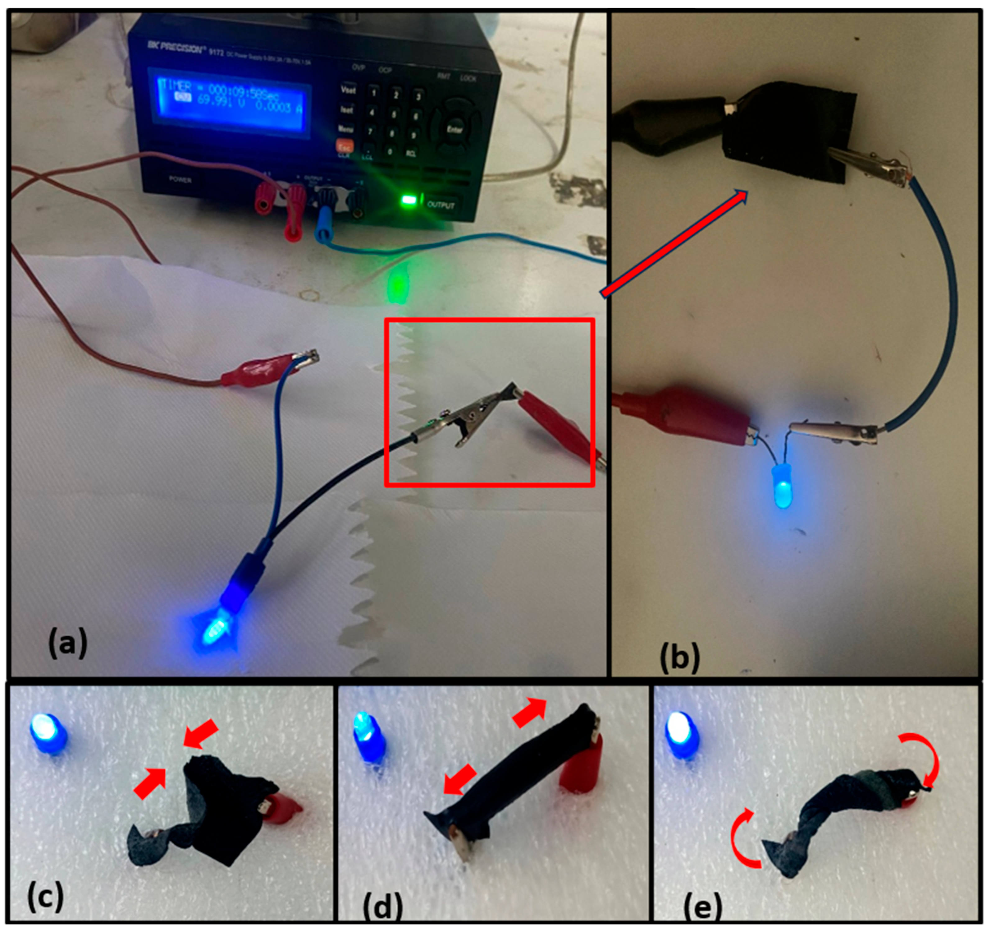
Vi-25%PANI-g-Chs was tested in a basic electrical circuit (Figure 12). The experimental setup comprised a precision voltage generator, an indicator LED, and the composite connected in series via alligator clips.

As illustrated in Figure 12a,b, the LED illuminates brightly when Vi-25%PANI-g-Chs is integrated into the circuit, directly confirming the electrical conductivity measured by the Hall effect. Remarkably, the LED maintains its illumination even when the composite undergoes various mechanical deformations, including stretching (Figure 12c), bending (Figure 12d), and twisting (Figure 12e), demonstrating exceptional conductive robustness under mechanical stress. This electrical stability under deformation not only validates the previously described conductivity measurements but also reveals the considerable potential of these materials for flexible electronics applications, where maintaining electrical properties under deformation is crucial. The continuity of electrical conduction during deformation suggests that the conductive network formed by PANI grafted onto chitosan and a Vinavil matrix preserves its structural integrity, which is essential for the development of wearable and deformable electronic devices.

Building upon the qualitative demonstrations of electrical conductivity under mechanical deformation (stretching), this study further evaluates the material’s potential as a high-performance strain sensor for applications in flexible electronics. Vi-25%PANI-g chitosan film (dimensions: 2 cm × 1 cm × 0.5 mm) was mounted between precision tweezers equipped with electrical contacts at each end. Controlled mechanical elongation was applied while simultaneously measuring the electrical resistance using an ohmmeter. The applied strain (ε) was calculated based on ε % = (L − L₀)/L₀ × 100%, where L represents the length and L₀ is the initial length, 2.0 cm (distance between clamps).

Table 6. Measured electrical resistance changes as a function of applied mechanical strain.

ε (%)	R (Ω)	∆R/R0 (%)
0	830	0
20	910	9.6
40	1020	22.8
80	1200	44.6
100	1530	84.3

summarizes the measured electrical resistance changes as a function of the applied mechanical strain.

The data validates the material’s conductive robustness, previously demonstrated through LED illumination during mechanical deformation, and provides the essential quantitative foundation for its development as a strain and motion sensing element for applications in flexible electronics.

4. Conclusions

This study successfully developed a novel nanocomposite material obtained via simple oxidative polymerization, based on Vinavil and PANI-g-Chs, for applications in flexible electronics. For comparison, Vi-PANI was also studied.

The core–shell structure shown by PANI-g-Chs combines the biocompatibility and structural stability of chitosan with the electrical conductivity of PANI, making it a promising candidate for controlled delivery systems, conductive composites, and advanced electrochemical applications.

Moreover, the grafted polymer creates a three-dimensional interconnected network that simultaneously reinforces the structural and electrical integrity of the material.

Compared with pristine PANI, PANI grafted onto chitosan results in improved dispersion, more uniform conductive films, and substantially increased electrical properties.

Key achievements include a higher conductivity of 77.79 S/m, improved charge carrier mobility (1162.7 cm²/V·s), and enhanced mechanical flexibility, with a 300% increase in the storage modulus with respect to Vi-PANI. Finally, the composite material was tested as a flexible conductive circuit for LED illumination under mechanical stress. The obtained results position Vi-PANI-g-Chs nanocomposites as a promising platform for wearable electronics, biomedical sensors, and eco-friendly conductive devices, bridging the gap between performance and environmental sustainability. Future work could explore large-scale production, long-term stability, and integration into multifunctional devices to advance real-world applications.