Article

Universal Expressions for the Polarization and the Depolarization Factor in Homogeneous Dielectric and Magnetic Spheres Subjected to an External Field of Any Form

by
Dimosthenis Stamopoulos
Department of Physics, School of Science, National and Kapodistrian University of Athens, Zografou Panepistimioupolis, 15784 Athens, Greece
Crystals 2025, 15(4), 331; https://doi.org/10.3390/cryst15040331
Submission received: 28 February 2025 / Revised: 28 March 2025 / Accepted: 28 March 2025 / Published: 30 March 2025

Abstract

:
Spherical structures of dielectric and magnetic materials are studied intensively in basic research and employed widely in applications. The polarization, Crystals 15 00331 i003 (P for dielectric and M for magnetic materials), is the parent physical vector of all relevant entities (e.g., moment, Crystals 15 00331 i004, and force, F), which determine the signals recorded by an experimental setup or diagnostic equipment and configure the motion in real space. Here, we use classical electromagnetism to study the polarization, Crystals 15 00331 i003, of spherical structures of linear and isotropic—however, not necessarily homogeneous—materials subjected to an external vector field, Crystals 15 00331 i002 (Eext for dielectric and Hext for magnetic materials), dc (static), or even ac of low frequency (quasistatic limit). We tackle an integro-differential equation on the polarization, Crystals 15 00331 i003, able to provide closed-form solutions, determined solely from Crystals 15 00331 i002, on the basis of spherical harmonics, Y l m . These generic equations can be used to calculate analytically the polarization, Crystals 15 00331 i003, directly from an external field, Crystals 15 00331 i002, of any form. The proof of concept is studied in homogeneous dielectric and magnetic spheres. Indeed, the polarization, Crystals 15 00331 i003, can be obtained by universal expressions, directly applicable for any form of the external field, Crystals 15 00331 i002. Notably, we obtain the relation between the extrinsic, Crystals 15 00331 i005, and intrinsic, Crystals 15 00331 i007, susceptibilities ( χ e e x t and χ e i n t for dielectric and χ m e x t and χ m i n t for magnetic materials) and clarify the nature of the depolarization factor, Crystals 15 00331 i009, which depends on the degree l—however, not on the order m of the mode ( l , m ) of the applied Crystals 15 00331 i002. Our universal approach can be useful to understand the physics and to facilitate applications of such spherical structures.

1. Introduction

Dielectric and magnetic spherical structures in the form of non-thick hollow shells and compact spheres, whether homogeneous, continuously nonhomogeneous, or layered, are studied widely in the last decades in terms of both basic research and applications. Dielectric spherical structures are used in scattering applications and shielding/invisibility cloaks [1,2,3,4,5] to model biological cells during sorting, i.e., dielectrophoresis, focusing, and manipulation applications, and to describe the micromanipulation and controlled assembly of colloidal particles [6,7,8,9,10,11,12] in energy applications [13,14] and in polymers science [15]. Also, biological cells subjected to electric fields are commonly modeled by dielectric spheres [16,17,18,19,20]. Magnetic spherical structures are employed in many applications, as well—to name just a few, catalysis [21,22]; environment, e.g., water purification [23,24,25]; and shielding/invisibility cloaks [26,27,28]. Also, their utilization is extensive in biomedicine [29,30,31,32], namely, magnetic and immunomagnetic sorting, i.e., magnetophoresis; manipulation and/or delivery of cells [33,34,35,36,37,38,39,40,41,42,43,44,45]; diagnostic radiology, e.g., in Magnetic Resonance Imaging, Positron Emission Tomography, and Single-Photon Emission Computed Tomography [46,47,48,49,50,51]; and therapy, e.g., blood purification [52,53,54,55,56,57] and hyperthermia [58,59,60,61,62,63].
In all these cases, the polarization, Crystals 15 00331 i003, that is, P for dielectric and M for magnetic materials, is the vector entity of interest since it reflects the endogenous properties of the material [64,65,66,67,68,69]. For instance, the estimation of the polarization, Crystals 15 00331 i003, is crucial since the bound charge densities of volume and surface origin can be obtained directly through ρb(r) = Crystals 15 00331 i003 (r) and σb(r)|s = Crystals 15 00331 i003 (r)∙ n ^ |s, respectively. In line with this fact, all relevant vector entities, that is, moment, Crystals 15 00331 i004, force, F, and torque, T, can be obtained analytically when the polarization, Crystals 15 00331 i003, is known. These vectors are important for basic research and of paramount interest for all applications since they ultimately determine the signals recorded by an experimental setup (e.g., ac magnetic susceptibility, vibrating sample magnetometry, torque magnetometry, etc.; see [70,71] and references therein) or diagnostic equipment (e.g., magnetic resonance imaging) and configure the motion of the spherical structures in real space (e.g., dielectrophoresis, magnetophoresis, microfluidic devices; see [6,7,8,9,10,11,12,33,34,35,36,37,38,39,40,41,42,43,44,45] and references therein).
Here, we focus on the polarization, Crystals 15 00331 i003, and the counteracting depolarization factor (see [72,73,74] for electric depolarization and [74,75,76,77] for magnetic depolarization) of spherical structures of linear and isotropic—however, not necessarily homogeneous—materials when subjected to an external vector field, Crystals 15 00331 i002, of any form (Eext for dielectric and Hext for magnetic materials). We stress that knowing the theoretical dependence of the polarization, Crystals 15 00331 i003, on the (total) field, Crystals 15 00331 i006, (E for dielectric and H for magnetic materials) is practically useless, since in most cases, Crystals 15 00331 i006 cannot be measured at the interior of a specimen. What really makes sense is the Crystals 15 00331 i003-Crystals 15 00331 i002 equation since the characteristics of both vectors are known to the user; during the experiment, the cause, Crystals 15 00331 i002, is predetermined at will, while the result, Crystals 15 00331 i003, is measured either directly or indirectly by means of dc or ac susceptibility. Here, we derive a universal equation for the polarization, Crystals 15 00331 i003, originating exclusively from the external field, Crystals 15 00331 i002, applied by the user, which can be of any form. We also derive a reliable relation between the extrinsic, Crystals 15 00331 i005, and intrinsic, Crystals 15 00331 i007, susceptibilities ( χ e e x t and χ e i n t for dielectric and χ m e x t and χ m i n t for magnetic materials), where Crystals 15 00331 i003~Crystals 15 00331 i005Crystals 15 00331 i002 and Crystals 15 00331 i003~Crystals 15 00331 i007Crystals 15 00331 i006, respectively. Accordingly, we are able to translate the experimentally measured extrinsic susceptibility, Crystals 15 00331 i005, of each particular specimen to the intrinsic susceptibility, Crystals 15 00331 i007, of the parent material for the cases where a dc or an ac field of low frequency is applied (static and quasistatic case, respectively).
Once these equations are obtained, we focus on homogeneous dielectric and magnetic spheres to document the proof of concept. In this case, we are able to obtain stand-alone equations of the polarization, Crystals 15 00331 i003, from an external field, Crystals 15 00331 i002, of any form and to clarify the nature of the depolarization factor, Crystals 15 00331 i009, appearing in the relation between Crystals 15 00331 i005 and Crystals 15 00331 i007. These universal, stand-alone formulas on Crystals 15 00331 i003 are ready to use for both dielectric and magnetic materials for all relevant cases; thus, they facilitate the understanding of underlying physics and the realization of useful applications.

2. Background

Our aim is to find a universal equation for the polarization, Crystals 15 00331 i003(r), of a spherical structure, either dielectric or magnetic, of known characteristics, in respect to an external field, Crystals 15 00331 i002(r), of any form. In all applications discussed above, the external field, Crystals 15 00331 i002(r), which induces the polarization, Crystals 15 00331 i003(r), stems from sources placed outside the spherical structure. Figure 1 shows an illustration of this case in its general form, referring equally well either to a dielectric or a magnetic material. A spherical structure (e.g., compact sphere, hollow spherical shell, etc.)—linear and isotropic; however, not necessarily, homogeneous—is constructed of a parent material with intrinsic susceptibility Crystals 15 00331 i007 ( χ e i n t for a dielectric, 0 χ e i n t < , and χ m i n t for a magnetic, 1 χ m i n t < , material). The spherical structure hosts the origin of the coordinate system at its center. As shown, it is subjected to an external field, Crystals 15 00331 i002(r), of known characteristics, applied by the user, where Crystals 15 00331 i002(r) refers to the external electric, Eext(r), and magnetic, Hext(r), field for a dielectric and a magnetic material, respectively. The source of Crystals 15 00331 i002(r), called primary (else, free electric charge and magnetic pseudocharge, respectively), is placed outside the spherical structure. The color employed in the spherical structure is only indicative of the intensity of the secondary source (else, bound electric charge and magnetic pseudocharge), which initially is induced as a response to Crystals 15 00331 i002(r) (transient stage) [68,69]. However, the secondary source produces the internal field, Crystals 15 00331 i008(r), which refers to the internal electric, Eint(r), and magnetic, Hint(r), field for a dielectric and a magnetic material, respectively. Then, Crystals 15 00331 i008(r) adds to Crystals 15 00331 i002(r) to result in the (total) field, Crystals 15 00331 i006(r), from which the secondary source ultimately depends (steady state) [68,69]. The established polarization, Crystals 15 00331 i003(r), refers to the electric, P(r), and magnetic, M(r), polarization, for a dielectric and a magnetic material, respectively. Formally, the polarization, Crystals 15 00331 i003(r), relates to Crystals 15 00331 i006(r) through Crystals 15 00331 i003(r)~Crystals 15 00331 i007(r)Crystals 15 00331 i006(r), where Crystals 15 00331 i007(r) is the intrinsic susceptibility, an endogenous property of the parent material ( P ( r ) = ε 0 χ e i n t ( r ) E ( r ) and M ( r ) = χ m i n t H ( r ) , respectively). However, a relation between the polarization, Crystals 15 00331 i003(r), and the external field, Crystals 15 00331 i002(r), is more convenient in every sense [70]. In this case, Crystals 15 00331 i003(r)~Crystals 15 00331 i005(r)Crystals 15 00331 i002(r), where now Crystals 15 00331 i005(r) is the extrinsic susceptibility, an exogenous property of the spherical structure employed in each particular case ( P ( r ) = ε 0 χ e e x t E e x t ( r ) and M ( r ) = χ m e x t H e x t ( r ) , respectively). Notably, the internal field, Crystals 15 00331 i008(r), produced by the secondary source acts against the polarization; it associates to the depolarization of the spherical structure through the so-called depolarization factor, Crystals 15 00331 i009 (see below). The latter is defined through the constitutive relation between Crystals 15 00331 i005(r) and Crystals 15 00331 i007(r) [68,69,70,72,73,74,75,76,77].
In general, the external scalar potential (either electric or magnetic), Crystals 15 00331 i001(r), originating from the primary source can be expanded on the basis of spherical harmonics (SHs) in a regime free of any source, based on the solution of the Laplace equation. It should be clarified that Crystals 15 00331 i001(r) is solely the external scalar potential originating from the primary source, so that it does not include the contribution of any secondary sources. The latter are developed at the spherical structure due to its limited size in the form of bound charge densities, volume ρb(r) = Crystals 15 00331 i003 (r) and surface σb(r)|s = Crystals 15 00331 i003 (r)∙ n ^ |s ones, and produce the internal scalar potential, Crystals 15 00331 i010(r), which adds to Crystals 15 00331 i001(r), ultimately resulting in the (total) scalar potential, Crystals 15 00331 i011(r). Here, our aim is to find a universal, ready-to-use equation of Crystals 15 00331 i003 (r) when only the external scalar potential/vector field, Crystals 15 00331 i001(r)/Crystals 15 00331 i002(r), are known (i.e., without knowing the total Crystals 15 00331 i011(r)/Crystals 15 00331 i006(r)). Notably, Crystals 15 00331 i001(r)/Crystals 15 00331 i002(r) can have any form. This is why we call the equation of Crystals 15 00331 i003 (r) in respect to Crystals 15 00331 i001(r)/Crystals 15 00331 i002(r) universal; once we know such an equation of Crystals 15 00331 i003 (r), there is no need to solve each problem in a step-by-step fashion by using the conventional approach (Laplace equation, multipole expansion, method of images/inversion, satisfying the boundary/interface conditions, etc.). Below, we refer to the case of electricity. The relevant results of magnetism can be easily inferred.

3. Dielectric Spherical Structure Subjected to an External Electric Scalar Potential/Vector Field of Any Form

Here, we refer to the case of a dielectric spherical structure of radius a, subjected to an external electric scalar potential/vector field, U e x t r / E e x t ( r ) , of any form. The latter are produced by a free source placed outside the spherical structure, as shown in Figure 1. The dielectric parent material of which the spherical structure is constructed is linear and isotropic, however, not necessarily homogeneous. According to the Laplace equation, the external scalar potential has the form [65,66,78]
U e x t r = l = 0 m = l l ( A l m r l + B l m r l + 1 ) Y l m ( θ , φ )
where the SH are determined by
Y l m θ , φ = 2 l + 1 4 π l m ! l + m ! P l m c o s θ e i m φ
Since in all real-life applications discussed here, the primary/free source is placed outside the spherical structure, the expression of U e x t ( r ) refers to the inside space; thus, the term B l m r l + 1 should be omitted by setting B l m = 0 for all values of (l,m). Under these conditions, the external scalar potential at the interior of the spherical structure (area of interest) reads
U e x t r = l = 0 m = l l A l m r l Y l m ( θ , φ )
where we can define the general term of the expansion through
U l , e x t m r = A l m r l Y l m ( θ , φ )
so that
U e x t r = l = 0 m = l l U l , e x t m r
while the coefficients A l m are formally obtained through the equation
A l m = 1 r l 0 2 π 0 π U e x t r Y l m * θ , φ s i n θ d θ d φ
First, we stress that for the case discussed here, the value l = 0 is not considered since it returns a null output; the term l , m = 0,0 refers to a constant external scalar potential, U 0 , e x t 0 r = A 0 0 r 0 Y 0 0 ( θ , φ ) , so that the respective field is zero, E 0 , e x t 0 r = 0 . However, at present, we do not reject this value. We come back to this issue when the final equations are obtained. Second, in this equation, U e x t r obviously obeys the separation of variables, U e x t r ~ U e x t r U e x t θ U e x t φ , so that its radial component, U e x t r , can be brought out of the integral to restore the fact that the coefficients A l m are constants (the term 1 / r l is always eliminated by U e x t r ). However, we do not decompose U e x t r in Equation (6); its native, complete expression met in every different case is introduced in Equation (6) to always verify the validity of the obtained results (see below). Third, Y l m * θ , φ is the complex conjugate of Y l m θ , φ [65,66,78].
Once we have determined the form of the external scalar potential, U e x t r , produced by the primary/free source, we now consider the dielectric spherical structure for the case of a linear, isotropic and homogeneous dielectric material of intrinsic susceptibility, χ e i n t . From the constitutive relation between the polarization and electric field, we have
P r = ε 0 χ e i n t E ( r )
Once
E r = E e x t r + E i n t ( r )
we obtain
P r = ε 0 χ e i n t E e x t r + ε 0 χ e i n t E i n t ( r )
where the external and internal components of the electric field are determined by the respective component of the scalar potential through
E e x t r = U e x t r
and
E i n t r = U i n t r
Notably, while E e x t r polarizes the specimen, E i n t r acts toward its depolarization [68,69,70,72,73,74,75,76,77]. Indeed, E e x t r and E i n t r relate to the polarization, P r , through the equations
E e x t r = ε 0 χ e i n t 1 + N χ e i n t 1 P r
and
E i n t r = ε 0 N 1 P r
The minus sign in the second equation dictates that E i n t r tends to depolarize the specimen; the higher the depolarization factor, N , the stronger the depolarization.
The internal scalar potential, U i n t r , can be easily obtained through the secondary/bound sources by using the generalized law of Coulomb [66,68]
U i n t r = 1 4 π ε 0 V ρ b ( r ) | r r | d V + 1 4 π ε 0 S σ b ( r ) | r r | d S
else
U i n t r = 1 4 π ε 0 V · P ( r ) | r r | d V + 1 4 π ε 0 S P ( r ) · n ^ | r r | d S
In what follows, we focus on homogeneous dielectric and magnetic spheres, so that the volume integral in Equation (15) is omitted since · P r = 0 . The surface integral can be modified based on the multipole expansion on the basis of SH. Since we are interested in finding the polarization at the interior of a dielectric and magnetic homogeneous sphere, and the surface secondary/bound charge resides at the border of this volume, we employ the expansion of | r r | 1 for the inside space ( r < r ), presented by [65,66,68,78]
1 | r r | = 4 π l = 0 m = l l 1 2 l + 1 r l r l + 1 Y l m ( θ , φ ) Y l m * θ , φ
where r and r run over the volume of the observation and secondary/bound source, respectively. By using the above Equations (15) and (16), we obtain
U i n t r = 1 ε 0 l = 0 m = l l 1 2 l + 1 r l Y l m ( θ , φ ) S P r · n ^ Y l m * θ , φ r l + 1 d S
We define the surface integral through the following equation
I l , s u r m = S P r · n ^ Y l m * θ , φ r l + 1 d S , r = a
Notice that I l , s u r m is a scalar constant. Thus, the above Equation (17) obtains the form
U i n t r = 1 ε 0 l = 0 m = l l 1 2 l + 1 I l , s u r m r l Y l m ( θ , φ )
In addition, through the above expression, Equation (11) obtains the form
E i n t r = 1 ε 0 l = 0 m = l l 1 2 l + 1 I l , s u r m r l Y l m θ , φ
Substituting this expression into Equation (9), we obtain
P r = ε 0 χ e i n t E e x t r χ e i n t l = 0 m = l l 1 2 l + 1 I l , s u r m r l Y l m θ , φ
Here, we may define
P e x t r = ε 0 χ e i n t E e x t r
the polarization of the dielectric induced solely by the external component of the electric field, thus termed external polarization. Note that P e x t r is a known vector since both χ e i n t and E e x t r are known. By using this definition, the above Equation (21) becomes
χ e i n t l = 0 m = l l 1 2 l + 1 I l , s u r m r l Y l m θ , φ + P r = P e x t r
This equation is the basis of our work. It is actually a nonhomogeneous integro-differential equation on P r . Most important, this equation can be considered as a non-local equation since P r depends on the values of its normal component, P ( r ) · n ^ , over the surface, S , of the dielectric, through the term I l , s u r m (Equation (18)). The left part contains unknowns, while the right part is known.
To tackle this equation, we need to reform its right side. From Equations (10) and (22), we have
P e x t r = ε 0 χ e i n t U e x t r
Also, by using Equations (4) and (5) for U e x t r , the above equation becomes
P e x t r = ε 0 χ e i n t l = 0 m = l l A l m r l Y l m θ , φ = l = 0 m = l l P l , e x t m r
where we have defined the general term of the expansion
P l , e x t m r = ε 0 χ e i n t A l m r l Y l m θ , φ
while the coefficients A l m are determined by Equation (6).
Now, we are able to consider a solution for P r in the form of an expansion
P r = l = 0 m = l l P l m r
The general term of the series should be obtained through
P l m r = C l m P l , e x t m r
where the coefficients C l m are unknowns that should be determined (see below).
Substituting P l , e x t m r from Equation (26), we obtain
P l m r = ε 0 χ e i n t C l m A l m r l Y l m θ , φ
Thus, Equation (27) becomes
P r = ε 0 χ e i n t l = 0 m = l l C l m A l m r l Y l m θ , φ
Once we have at hand a possible solution for P r , we are able to return to the respective nonhomogeneous and non-local integro-differential equation. Accordingly, by using Equations (25) and (30), Equation (23) obtains the form
l = 0 m = l l I l , s u r m 2 l + 1 ε 0 C l m A l m + ε 0 A l m r l Y l m θ , φ = 0
To proceed, we should calculate I l , s u r m from Equation (18) (see below). As we prove here, for the case of homogeneous dielectric and magnetic spheres, the mathematical management of this equation leads to universal, ready-to-use expressions for any form of the external electric scalar potential/vector field, U e x t r / E e x t ( r ) . Accordingly, once the above expansion should be valid at every point r = ( r , θ , φ ) of the interior of the dielectric sphere, the coefficients should be zero, I l , s u r m / ( 2 l + 1 ) ε 0 C l m A l m + ε 0 A l m = 0 , so that
C l m = 1 + 1 ε 0 1 2 l + 1 I l , s u r m A l m
This equation is important since it defines the desired coefficients C l m needed to construct the solution of the polarization, P r , through Equation (30). We recall that the coefficients A l m are known, calculated by Equation (6). Thus, only the surface integral I l , s u r m is still needed. This can be calculated as follows. Using Equation (30), after some algebraic calculations, Equation (18) becomes
I l , s u r m = ε 0 χ e i n t l = 0 m = l l C l m A l m l a l l 0 2 π 0 π Y l m θ , φ Y l m * θ , φ s i n θ d θ d φ
We note that the double summation runs over the values of ( l , m ) , determined by the form of each particular external scalar potential, U e x t r , since this will specify which coefficients A l m are zero or not through Equation (6). Once the surface integral, I l , s u r m , has been determined through Equation (33) and the desired expansion coefficients, A l m and C l m , have been calculated through Equations (6) and (32), respectively, the electric polarization, P r , can be obtained through Equation (30). Notably, the unknown coefficients C l m , determined by Equation (32), appear in Equation (33) of the surface integral, I l , s u r m , as well. Thus, by substituting Equation (33) into Equation (32), we obtain an algebraic equation, which should be solved to ultimately obtain the desired coefficients C l m for each particular case of the external scalar potential/vector field, U e x t r / E e x t r , applied to the homogeneous dielectric sphere.
From Equation (33), we see that the orthogonality equation of the SH [65,66,78] is finally obtained
0 2 π 0 π Y l m θ , φ Y l m * θ , φ s i n θ d θ d φ = δ l l δ m m
With simple algebraic calculations, we obtain for the surface integral
I l , s u r m = ε 0 χ e i n t C l m A l m l
where we recall that the known coefficients A l m are determined by Equation (6).
Substituting the above expression into Equation (32), we obtain
C l = 1 1 + l 2 l + 1 χ e i n t
We stress that we have dropped the upper index m from the coefficients C l m (that is, the original C l m is replaced by C l ) since, as evidenced from this equation, though they depend on the degree, l , they do not depend on the order, m , of the SH.
Once the coefficients C l have been determined, we are able to construct the solution of the polarization, P r , for the case of a homogeneous dielectric sphere discussed in this section. Indeed, Equation (30) becomes
P r = ε 0 χ e i n t l = 0 C l m = l l A l m r l Y l m θ , φ
where the coefficients A l m are determined by Equation (6), while the C l coefficients are determined by Equation (36).
Importantly, Equation (37) can be written in the slightly modified form
P r = ε 0 l = 0 χ e i n t C l m = l l A l m r l Y l m θ , φ
Now we are able to define
χ e , l e x t = χ e i n t C l = χ e i n t 1 + l 2 l + 1 χ e i n t
so that Equation (38) obtains the modified form
P r = ε 0 l = 0 χ e , l e x t m = l l A l m r l Y l m θ , φ
where the coefficients A l m are still determined by Equation (6).
By defining the general term
P l m r = ε 0 χ e , l e x t A l m r l Y l m θ , φ
we may conclude with the electric polarization in the compact form
P r = l = 0 m = l l P l m r
However, though obvious, the connection with the external vector field, E e x t r , is still missing. By recalling the general term of the expansion of U e x t r , Equation (3), and the fact that E r = U r holds, we can define the general term of the expansion of E e x t through
E l , e x t m r = A l m r l Y l m θ , φ
so that
E e x t r = l = 0 m = l l E l , e x t m r
A direct comparison between the general terms P l m r and E l , e x t m r , calculated by the above Equations (41) and (43), respectively, leads to
P l m r = ε 0 χ e , l e x t E l , e x t m r
This expression should be quite familiar to experts in the field. It relates the general term of the polarization to that of the external electric field. Thus, through Equation (45), we may fairly define χ e , l e x t as the extrinsic electric susceptibility of degree l of the specimen, in connection to the intrinsic electric susceptibility, χ e i n t , of the parent material [68,69,70,72,73,74]. Once we have defined the extrinsic electric susceptibility, χ e , l e x t , Equation (39) can be rewritten as
χ e , l e x t = χ e i n t 1 + N l χ e i n t
where we identified the depolarization factor of degree l through
N l = l 2 l + 1
The above equations are quite informative. First, notice that the value l = 0 (for which N l = 0) should not be considered since it refers to the null case of an external scalar potential/vector field, which is constant/zero (for l , m = ( 0,0 ) , we have U 0 , e x t 0 r = A 0 0 r 0 Y 0 0 ( θ , φ ) , so that E 0 , e x t 0 r = 0 ). Second, given that the term 2 l + 1 appears both in the normalization factor and in the addition theorem of SH, we understand that the depolarization factor of degree l , N l , can be considered as a ‘weighting factor’ of mode l over the 2 l + 1 available values of m . Third, both the extrinsic electric susceptibility, χ e , l e x t , Equation (46), and the depolarization factor of degree l , N l , Equation (47), are degenerate over the 2 l + 1 available values of order m of each specific mode with fixed degree l . This property stems from the fact that, in the case discussed here, the dielectric spherical structure is homogeneous; thus, it possesses symmetry in respect to rotations around the z-axis (its properties do not depend on angle φ). Fourth, the depolarization factor of each mode, N l , always ranges within 0 N l 1 for all 1 l < , as it should. Specifically, for the lowest possible value l = 1 , which refers to the simple case of an external homogeneous electric field applied to a homogeneous sphere of radius a and intrinsic electric susceptibility χ e i n t , we obtain the expected results N 1 = 1 / 3 and χ e , 1 e x t = χ e i n t / ( 1 + 1 / 3 χ e i n t ) (see below). In the other limiting case where l , we obtain N l = 1 / 2 and χ e , l e x t = χ e i n t / ( 1 + 1 / 2 χ e i n t ) . Thus, we conclude that for all 1 l < , the depolarization factor ranges within 1 / 3 N l 1 / 2 . Fifth, for a parent dielectric material with quite high χ e i n t 1 , the extrinsic susceptibility yields
χ e , l e x t ~ 2 l + 1 l = 1 N l
On the other hand, for a quite low χ e i n t 1 , the extrinsic susceptibility becomes
χ e , l e x t ~ χ e i n t
These observations are summarized in Figure 2a,b, which, based on Equation (46), present the function χ e , l e x t ( χ e i n t , l ) for χ e i n t , which ranges continuously within an extended range 0 χ e i n t 100 in panel (a) and a limited range 0 χ e i n t 3 in panel (b). In both panels (a) and (b), the degree l is surveyed for the distinct integer values within 1 l 10 . Sixth, from these data, we see that the value of the extrinsic susceptibility, χ e , l e x t , recorded in an experiment depends noticeably on the mode l of the external field, E l , e x t m r , applied to the specimen. Thus, if instead of an absolutely homogeneous external electric field, i.e., l = 1 , an admixture of l = 1 and of higher-order modes is applied to the specimen, the ultimately estimated extrinsic susceptibility, χ e , l e x t , can be quite wrong. For instance, consider a specimen with quite high χ e i n t . Its excitation with the mode l = 1 will result in χ e , 1 e x t ~ 3 , while its excitation with the mode l = 2 will yield χ e , 2 e x t ~ 2.5 , referring to a noticeable difference on the order of 16%. This can be inferred from both Equation (48) and the simulations presented in Figure 2a,b. Seventh, strictly speaking, the above analysis holds for the case where E e x t r is a dc field (static case). However, the results obtained above hold even for the case where E e x t r is a time–harmonic ac field of low frequency (quasistatic case), for instance, the spatially homogeneous E e x t r = E 0 c o s ( ω t ) . Thus, the results obtained here can be directly implemented in many applications.
To summarize, for the case of a homogeneous spherical structure (linear and isotropic, as well) of radius a and intrinsic electric susceptibility, χ e i n t , subjected to an external electric scalar potential/vector field, U e x t r / E e x t r , of the generic form determined by Equations (3)–(6)/(43), (44), and (6), the induced electric polarization, P r , is calculated by the universal Equations (40)–(42), while the extrinsic electric susceptibility of degree l , χ e , l e x t , is determined by Equation (46), and the depolarization factor of degree l , N l , is calculated by Equation (47). This information is the only needed for each case to calculate all relevant scalar and vector entities, such as the density of the bound charge induced onto the surface of the spherical structure; the depolarization/internal electric field produced at the interior of the spherical structure by the density of the bound charge residing at its surface; the moment of the spherical structure; and finally, the force and torque exerted onto the spherical structure by the external scalar potential/vector field.
Finally, some remarks are urgently needed here on these equations to assist understanding of their physical content and facilitate their use in practice. First, notice that for the case discussed here, where the primary/free sources are placed outside the area of interest (outside the spherical structure), the lowest meaningful value of degree l is l = 1 . The value l = 0 refers to the null case, where the external scalar potential is constant; thus, the external electric field is zero. Thus, in the above equations, the summations should actually start from l = 1 . Second, in the above equations, r is actually fixed at the surface of the spherical structure of radius a. Thus, at the end of all mathematical operations, we have to simply replace r = a . Accordingly, to find the polarization electric, P r , by using Equation (40), we follow the next steps: (i) we determine the values of indices ( l , m ) , over which the summations should run through to identify the nonzero coefficients A l m by using Equation (6); (ii) we construct the respective terms r l Y l m θ , φ , calculate their gradient r l Y l m θ , φ , and multiply by the respective coefficient A l m to obtain all relevant terms A l m r l Y l m θ , φ ; (iii) for each fixed value of degree l , we calculate the sum of all terms over the different values of order m ; and (iv) we take into account each term of degree l of the extrinsic electric susceptibility, χ e , l e x t , and calculate the summation over the different values of degree l . At the end of this algebraic calculation, we have to simply replace r = a . Third, though the employed SH are complex functions, the electric polarization, P r , obtained through Equation (40) at the end of the algebraic steps described above, should be a real vector. This is clarified in Appendix A. To facilitate the use of Equation (40), in Appendix B, we present the SH, Y l m θ , φ , together with the gradient, r l Y l m θ , φ , for the degree up to l = 2 . The proof of concept of the mathematical methodology presented above, based on Equation (40), is clarified with some representative problems discussed in Appendix C.

4. Magnetic Spherical Structure Subjected to an External Magnetic Scalar Pseudopotential/Vector Field of Any Form

Here, we refer to the relative case of a magnetic spherical structure of radius a, subjected to an external magnetic scalar pseudopotential/vector field, U m , e x t r / H e x t ( r ) . Again, the latter are produced by a free source (e.g., magnetic pseudocharges) placed outside the spherical structure, as shown in Figure 1. The magnetic parent material of which the spherical structure is constructed is linear and isotropic—however, not necessarily homogeneous. We can follow the exact same procedure to calculate all equations obtained above for the case of the dielectric sphere. Below, we briefly focus on the case of a homogeneous magnetic sphere. We only have to calculate the surface integral of Equation (33) for the case of magnetism studied here
I l , m , s u r m = χ m i n t l = 0 m = l l C l m A l , m m l a l l 0 2 π 0 π Y l m θ , φ Y l m * θ , φ s i n θ d θ d φ
We easily arrive at the following equations:
χ m , l e x t = χ m i n t 1 + N l χ m i n t
which defines the extrinsic magnetic susceptibility of degree l ,
N l = l 2 l + 1
which defines the depolarization factor of degree l , and
M r = l = 0 χ m , l e x t m = l l A l , m m r l Y l m θ , φ
which defines the magnetic polarization (i.e., magnetization). The necessary coefficients A l , m m are obtained through the equation
A l , m m = 1 r l 0 2 π 0 π U m , e x t r Y l m * θ , φ s i n θ d θ d φ
where
U m , e x t r = l = 0 m = l l A l , m m r l Y l m ( θ , φ )
is the known external magnetic pseudopotential applied by the user, in the form of an expansion on the basis of SH. As was discussed for the case of the dielectric sphere, here, we clarify that U m , e x t r obviously obeys the separation of variables, U m , e x t r ~ U m , e x t r U m , e x t θ U m , e x t φ , so that its radial component, U m , e x t r , can be brought out of the integral to restore the fact that the coefficients A l , m m are constants (the term 1 / r l is always eliminated by U m , e x t r ). Thus, when we substitute U m , e x t r in Equation (54), the obtained coefficients A l , m m are finally expansion constants, as expected.
Strictly speaking, the above results hold for the case where H e x t r is a dc field (static case). However, the results obtained above hold even for the case where H e x t r is a time–harmonic ac field of low frequency (quasistatic case), for instance, the spatially homogeneous H e x t r = H 0 c o s ( ω t ) . Thus, the results obtained here can be directly implemented in many applications for the case of magnetism.

5. Applicability of the Present Results and Perspectives

For the case of a single homogeneous dielectric sphere, the outcome of the present work is summarized by Equations (40), (46) and (47), aided by Equations (3) and (6). Specifically, Equations (3) and (6) should be used first to expand the external potential, U e x t r , on the basis of SH, Y l m . This enables us to identify the nonzero coefficients, A l m , and define the valid values of degree, l, and order, m, that are of mode ( l , m ) . Then, Equations (40), (46) and (47) can be readily used to directly obtain the polarization, P r , the extrinsic electric susceptibility, χ e , l e x t , and the depolarization factor, N l , of the single homogeneous dielectric sphere. In analogy, for a single homogeneous magnetic sphere, Equations (51)–(55) should be used in the same context.
Under specific circumstances, the above theoretical argumentation and the obtained equations hold even for the case of an assembly of homogeneous spheres, placed in a vacuum or even embedded in a host medium. Let us discuss this issue in some detail for the dielectric case; the magnetic one is entirely analogous. First, recall that secondary/bound sources reside solely at the surface of the dielectric sphere with the density σ b r = P ( r ) · n ^ | r = a . The density of the volume ones is zero, ρ b ( r ) = · P r = 0 . Second, these surface secondary/bound sources, σ b r , produce at the exterior of the homogeneous dielectric sphere the respective internal potential/field, U i n t o u t r / E i n t o u t r , where the upper index ‘out’ denotes the exterior (outside: out) of the sphere. Once we have at hand the electric polarization, Equation (40), the surface density of secondary/bound sources can be obtained through σ b r = P ( r ) · n ^ | r = a . After some relatively simple algebra, we obtain the equation
σ b r = ε 0 a l = 0 χ e , l e x t l m = l l A l m ( Ω ) Y l m θ , φ
where the extrinsic electric susceptibility, χ e , l e x t , is determined by Equation (46). The coefficients, A l m ( Ω ) , are obtained through the equation
A l m ( Ω ) = 0 2 π 0 π U e x t a , θ , φ Y l m * θ , φ s i n θ d θ d φ
where notice that the external potential is now fixed at r = a , that is, U e x t a , θ , φ . Then, the internal potential produced by σ b r at the outside space, U i n t o u t r , can be obtained by using the multipole expansion. After simple algebraic calculations, we obtain the equation
U i n t o u t r = l = 0 χ e , l e x t N l a r l + 1 m = l l A l m ( Ω ) Y l m θ , φ
where N l is the depolarization factor, Equation (47), and the coefficients, A l m ( Ω ) , are determined by the above Equation (57).
This expression satisfies the continuity of the scalar potential at the interface, r = a , between the dielectric sphere and the free space. Indeed, from Equations (19), (35), (36), (39), (46) and (47), we obtain the internal potential produced by σ b r at the inside space, U i n t i n r , determined from the equation
U i n t i n r = l = 0 χ e , l e x t N l r l m = l l A l m Y l m θ , φ
where the coefficients, A l m , are calculated by the standard Equation (6). The above equation can be rewritten in the form
U i n t i n r = l = 0 χ e , l e x t N l r a l m = l l A l m ( Ω ) Y l m θ , φ
where, now, the coefficients, A l m ( Ω ) , are calculated by the above Equation (57). From Equations (58) and (60), we can easily check that at the interface, r = a , the condition U i n t o u t a , θ , φ = U i n t i n a , θ , φ is satisfied.
Now, we are able to discuss the conditions under which the present study can be applied not only to a single homogeneous dielectric sphere but even for the case of an assembly of such units, placed in a vacuum or even embedded in a host medium. The assembly of the dielectric spheres can refer to different situations, for instance, to a homogeneous dispersion with a mean distance, < d s s > , (amorphous dispersion), and to a periodic placement with an exact distance, d s s , (crystal lattice). Obviously, the internal potential produced by the surface density, σ b r , of each unit at the outside space, U i n t o u t r , Equation (58), is of interest since this will determine the interaction between neighboring dielectric spheres. The important length scales, which should be considered on a comparative basis, are the ranges of U i n t o u t r and < d s s > or d s s , whether we have an amorphous dispersion or a crystal lattice. In this respect, Equation (58) can be rewritten in the form
U i n t o u t r = l = 0 m = l l U i n t o u t l m r
where the general term, U i n t o u t l m r , of each mode ( l , m ) is obtained through the equation
U i n t o u t l m = χ e , l e x t N l a r l + 1 A l m ( Ω ) Y l m θ , φ
The appearance of the SH, Y l m θ , φ , in the general term, U i n t o u t l m r , both directly and indirectly through the expansion coefficients, A l m ( Ω ) , reveals that for the constant degree, l , there is information on some primary directions/orientations, which depend on the order, m . This is important when a crystal lattice having a specific configuration is considered. Also, keeping in mind that we refer to the outside space, ( a / r ) < 1 , it directly becomes apparent that the leading mode of the maximum range, R m a x , is the dipolar one with l , m = 1 , 1 , 1,0 , and 1,1 . Let us denote the range of each of these modes as R l m . Then, R l m should be compared to < d s s > or d s s , depending on the occasion. Obviously, when R l m is lower than < d s s > or d s s , the distinct dielectric spheres do not interact, so that we have an assembly of isolated units, and the results of the present study can be directly applied. On the other hand, when R l m becomes on the order of < d s s > or d s s , the interaction among neighboring units cannot be neglected. Finally, when R l m exceeds < d s s > or d s s , the interaction includes more than first neighbors.
The above considerations cannot be developed further on a general basis. They can be employed à la carte, depending on the specific form of the external potential/field, U e x t r / E e x t r , applied to the system of dielectric spheres under consideration, since the specific U e x t r / E e x t r will define the modes l , m and the respective expansion coefficients, A l m ( Ω ) . Once this information is known, each range R l m can be calculated and compared to < d s s > or d s s , depending on the occasion. Finally, our expressions depend on the intrinsic properties of the dielectric sphere (radius, a , and intrinsic electric susceptibility, χ e i n t ). Thus, they can be employed to tackle the case where an assembly of dielectric spheres is not monodisperse in respect to these properties. For instance, when the assembly includes two subpopulations of a different radius, let us say, a and b , and/or intrinsic electric susceptibilities, χ e , a i n t and χ e , b i n t , our formulation can be employed to clarify the situation. Again, this issue cannot be considered further on a general basis. It can be studied à la carte, depending on the specific form of the external potential/field, U e x t r / E e x t r , applied to the assembly of dielectric spheres under consideration. These issues can be addressed in a future work.

6. Conclusions

Here, we introduced a new methodology for the calculation of the polarization, P, in dielectric (P) and magnetic (M) spherical structures of linear and isotropic—however, not necessarily homogeneous—parent materials. We constructed a non-local integro-differential equation and obtained universal solutions for the polarization, Crystals 15 00331 i003, that are applicable for any form of the external scalar potential/vector field, Crystals 15 00331 i001/Crystals 15 00331 i002 ( U e x t r /Eext for dielectric and U m , e x t r / H e x t ( r ) for magnetic materials). The proof of concept was assessed in homogeneous spheres subjected to an external scalar potential/vector field, Crystals 15 00331 i001/Crystals 15 00331 i002, of any form. In connection to the universal solutions of the polarization, Crystals 15 00331 i003, in respect to Crystals 15 00331 i002, we obtained a constitutive equation between the extrinsic, Crystals 15 00331 i005, and intrinsic, Crystals 15 00331 i007, susceptibilities ( χ e e x t and χ e i n t for dielectric and χ m e x t and χ m i n t for magnetic materials) and clarified the nature of the depolarization factor, Crystals 15 00331 i009, which, for the homogeneous case, exhibits a degeneracy on the order m of the mode ( l , m ) of the external scalar potential/vector field, Crystals 15 00331 i001/Crystals 15 00331 i002. Though, here, we have considered the static case of dc Crystals 15 00331 i001/Crystals 15 00331 i002, the obtained results hold even for the quasistatic case of a low-frequency ac Crystals 15 00331 i001/Crystals 15 00331 i002. Except for understanding the underlying physics, our approach can assist the evolution of static and quasistatic applications of dielectric and magnetic spherical structures since the polarization, Crystals 15 00331 i003, is the parent of all relevant entities (secondary/bound sources, ρ b and σ b , moment, Crystals 15 00331 i004, force, F, and torque, T), which determine the signals recorded by an experimental setup or diagnostic equipment and configure the motion in real space.

Funding

This research received no external funding.

Data Availability Statement

The data that support the findings of this study are available within the article.

Conflicts of Interest

The author declares no conflicts of interest.

Appendix A

Equation (40) in all cases should result in a real vector for the polarization, P r . Here, we obtain an equivalent form of this equation, which clarifies this issue. Properties of SH used here can be found in [65,66,78]. In Equation (40), the index of order m runs on both negative and positive values of degree l . Then, each pair l , m and ( l , m ) of the summation over the order m becomes
A l m r l Y l m θ , φ + A l m r l Y l m θ , φ
The SH obey the following property
Y l m θ , φ = ( 1 ) m Y l m * θ , φ
Starting from Equation (6), the coefficients A l m behave as follows
A l m = 1 r l 0 2 π 0 π U e x t r Y l m * θ , φ s i n θ d θ d φ
else
A l m = 1 r l 0 2 π 0 π U e x t r Y l m * θ , φ s i n θ d θ d φ
else
A l m = 1 r l 0 2 π 0 π U e x t r ( 1 ) m Y l m θ , φ s i n θ d θ d φ
else
A l m = ( 1 ) m 1 r l 0 2 π 0 π U e x t r Y l m θ , φ s i n θ d θ d φ
else
A l m * = ( 1 ) m 1 r l 0 2 π 0 π U e x t r Y l m * θ , φ s i n θ d θ d φ
Thus,
A l m * = ( 1 ) m A l m
so that
A l m = ( 1 ) m A l m *
Now we are ready to proceed with the calculation of each pair
A l m r l Y l m θ , φ + ( 1 ) m A l m * r l Y l m θ , φ
else
A l m r l Y l m θ , φ + A l m * r l ( 1 ) m Y l m θ , φ
else
A l m r l Y l m θ , φ + A l m * r l ( 1 ) m Y l m θ , φ
else
A l m r l Y l m θ , φ + A l m * r l Y l m * θ , φ
else
r l A l m Y l m θ , φ + A l m * Y l m * θ , φ
The part of the function that depends on the angles θ and φ (inner parenthesis) becomes
A l m Y l m θ , φ + A l m Y l m θ , φ *
which is always real.
Substituting this finding into Equation (40) and isolating the terms with m = 0 as a separate series, we obtain
P r = ε 0 l = 0 χ e , l e x t A l 0 r l Y l 0 θ , φ ε 0 l = 1 χ e , l e x t m = 1 l r l A l m Y l m θ , φ + A l m Y l m θ , φ *
Obviously, this equation guarantees that the obtained polarization, P r , is always a real vector.
The pair of Equation (A15) can be rewritten, as well, as follows
A l m Y l m θ , φ + A l m Y l m θ , φ * = 2 R A l m Y l m θ , φ
where R refers to the real part of the bracket.
Thus, the above Equation (A16) takes the equivalent form
P r = ε 0 l = 0 χ e , l e x t A l 0 r l Y l 0 θ , φ ε 0 l = 1 χ e , l e x t m = 1 l r l 2 R A l m Y l m θ , φ
Notice that in both Equations (A16) and (A18) of the polarization, P r , the summation over the order m runs only on the positive values, 1 m l (notice the appearance of the multiplying factor 2 in Equation (A18)).
Finally, we proceed with a slightly modified version of Equation (A18). We know that Y l 0 θ , φ has the form
Y l 0 θ , φ = 2 l + 1 4 π P l c o s θ
Also, the coefficients A l 0 obtain the form
A l 0 = A l = 2 l + 1 4 π 1 r l 0 2 π 0 π U e x t r P l c o s θ s i n θ d θ d φ
By using the above Equations (A19) and (A20), the polarization P r , Equation (A18), becomes
P r = ε 0 4 π l = 0 χ e , l e x t ( 2 l + 1 ) A l r l P l c o s θ 2 ε 0 l = 1 χ e , l e x t m = 1 l r l R A l m Y l m θ , φ
where now the coefficients A l are defined through
A l = 1 r l 0 2 π 0 π U e x t r P l c o s θ s i n θ d θ d φ
while the coefficients A l m are still defined through Equation (6), and the extrinsic electric susceptibility, χ e , l e x t , is still defined through Equation (46). We stress that the above Equation (A21) of the polarization, P r , is absolutely equivalent to Equation (40).
Some final remarks should be provided here on these equations to assist understanding of their physical content and facilitate their use in practice. First, notice that for the case discussed here, where the primary/free sources are placed outside the area of interest (outside the spherical structure), the lowest meaningful value of degree l is l = 1 . The value l = 0 refers to the null case, where the external scalar potential is constant; thus, the external electric field is zero. Thus, in the above equations, the summations should actually start from l = 1 . Second, notice that in these equations, the summation over the order m runs only on the positive values, 1 m l . Third, in the above equations, r is actually fixed at the surface of the spherical structure of radius a. Thus, at the end of all mathematical operations, we have to simply replace r = a . Accordingly, to find the polarization, P r , by using the above Equation (A21), we follow the next steps: Referring to the second, double summation over both the degree l and order m , (i) we determine the values of indices ( l , m ) , over which the summations should run through to identify the nonzero coefficients A l m by using Equation (6); (ii) we construct the respective terms r l R A l m Y l m θ , φ and calculate their gradient r l R A l m Y l m θ , φ ; (iii) for each fixed value of degree l , we calculate their sum over the different values of order m ; and (iv) we take into account each term of degree l of the extrinsic electric susceptibility, χ e , l e x t , and calculate the summation over the different values of degree l . Regarding the first, single summation over the degree l with the order fixed to m = 0 , the same rule of thumb should be applied. At the end of all these algebraic calculations, in both summations, we have to simply replace r = a .

Appendix B

To facilitate the use of Equation (40) for the calculation of the polarization, P r , from the external scalar potential, U e x t r , in Table A1 we provide the SH, Y l m θ , φ , together with the respective gradient r l Y l m θ , φ , for the degree up to l = 2 . This information can be directly substituted in Equation (40), thus bypassing the calculation of the desired gradient terms from scratch every time we handle a different external scalar potential/vector field, U e x t r / E e x t r . Below, the gradient terms are provided in two forms: a compact SH-based form and an equivalent trigonometric-based form.
Table A1. The SH, Y l m θ , φ , and the respective gradient r l Y l m θ , φ , for degree up to l = 2 .
Y l m (θ, φ) (rl Y l m (θ, φ))
Y 0 0 = 1 2 1 π 0
Y 1 1 = 1 2 3 2 π s i n θ e i φ
Y 1 1 r ^ 1 2 Y 1 0 e i φ θ ^ i 3 2 Y 0 0 e i φ φ ^
   else
1 2 3 2 π s i n θ e i φ r ^ 1 2 3 2 π c o s θ e i φ θ ^ i 1 2 3 2 π e i φ φ ^
Y 1 0 = 1 2 3 π c o s θ
Y 1 0 r ^ + 2 Y 1 1 e i φ θ ^
   else
1 2 3 π c o s θ r ^ 1 2 3 π s i n θ θ ^
Y 1 1 = 1 2 3 2 π s i n θ e i φ
Y 1 1 r ^ + 1 2 Y 1 0 e i φ θ ^ i 3 2 Y 0 0 e i φ φ ^
   else
1 2 3 2 π s i n θ e i φ r ^ + 1 2 3 2 π c o s θ e i φ θ ^ i 1 2 3 2 π e i φ φ ^
Y 2 2 = 1 4 15 2 π s i n 2 θ e 2 i φ
2 r Y 2 2 r ^ r Y 2 1 e i φ θ ^ i 5 r Y 1 1 e i φ φ ^
   else
2 r 1 4 15 2 π s i n 2 θ e 2 i φ r ^ + r 1 2 15 2 π s i n θ c o s θ e 2 i φ θ ^ + i r 1 2 15 2 π s i n θ e 2 i φ φ ^
Y 2 1 = 1 2 15 2 π s i n θ c o s θ e i φ
2 r Y 2 1 r ^ r 15 2 Y 0 0 e i φ 4 Y 2 2 e i φ θ ^ i 5 2 r Y 1 0 e i φ φ ^
   else
2 r 1 2 15 2 π s i n θ c o s θ e i φ r ^ r 1 2 15 2 π c o s 2 θ s i n 2 θ e i φ θ ^ i r 1 2 15 2 π c o s θ e i φ φ ^
Y 2 0 = 1 4 5 π ( 3 c o s 2 θ 1 )
2 r Y 2 0 r ^ + r 2 3 Y 2 1 e i φ θ ^
   else
2 r 1 4 5 π ( 3 c o s 2 θ 1 ) r ^ r 1 2 5 π s i n θ c o s θ θ ^
Y 2 1 = 1 2 15 2 π s i n θ c o s θ e i φ
2 r Y 2 1 r ^ + r 15 2 Y 0 0 e i φ 4 Y 2 2 e i φ θ ^ i 5 2 r Y 1 0 e i φ φ ^
   else
2 r 1 2 15 2 π s i n θ c o s θ e i φ r ^ + r 1 2 15 2 π c o s 2 θ s i n 2 θ e i φ θ ^ i r 1 2 15 2 π c o s θ e i φ φ ^
Y 2 2 = 1 4 15 2 π s i n 2 θ e 2 i φ
2 r Y 2 2 r ^ + r Y 2 1 e i φ θ ^ i 5 r Y 1 1 e i φ φ ^
   else
2 r 1 4 15 2 π s i n 2 θ e 2 i φ r ^ + r 1 2 15 2 π s i n θ c o s θ e 2 i φ θ ^ i r 1 2 15 2 π s i n θ e 2 i φ φ ^

Appendix C

Here, we assess the universal character of the mathematical methodology introduced in this work by exploring some representative examples for the case where the dielectric or magnetic sphere, of radius a is homogeneous with intrinsic electric and magnetic susceptibility, χ e i n t and χ m i n t , respectively. These data are summarized in Table A2 and Table A3 for the dielectric and magnetic sphere, respectively. The external free source, scalar potential, U e x t r and U m , e x t r , and vector field, E e x t r and H e x t r , are clearly shown at the upper part of each cell. The (total) scalar potential, U r and U m r , at the interior of the dielectric and magnetic sphere, obtained with conventional means (e.g., a step-by-step solution by using the Laplace equation, multipole expansion, or method of images/inversion), is also shown with appropriate referencing at the lower part of each cell. From the (total) scalar potential, U r and U m r , we obtain the relevant (total) vector field, E r and H r , through E r = U r and H r = U m r , respectively. Finally, we obtain the polarization, P r and M r , through the relevant constitutive equations, P r = ε 0 χ e i n t E r and M r = χ m i n t H r , respectively. The polarization of the dielectric, P r , and magnetic, M r , spheres, obtained directly with the universal equations introduced here, is shown in each case, as well. The results of the two methods are consistent.
Table A2. Representative cases of a homogeneous dielectric sphere subjected to an external electric scalar potential/vector field, U e x t r / E e x t r , produced by a primary/free source. The scalar potential, U r , obtained by using conventional methods of solution is shown. From U r , we can obtain E r and finally P r through E r = U r and P r = ε 0 χ e i n t E r , respectively. The result for P r obtained by using Equations (40)/(A21) introduced in this work is shown. The results obtained by the two methods are identical.
Representative Cases of a Homogeneous Dielectric Sphere Subjected to Uext(r)/Eext(r)
(C.1.1) Source: (a) opposite, large plates of a capacitor, placed at distance R > 2a, with surface density of free charge
σ f ± R / 2 = ε 0 E 0
or equivalently (b) spherical shell of radius R > a with surface density of free charge
σ f R , θ = 3 ε 0 E 0 c o s θ
External scalar potential, linear along the z-axis: U e x t r = E 0 z else U e x t r = E 0 r c o s θ
External vector field, uniform along the z-axis: E e x t r = E 0 z ^ .
Results
Scalar potential at the interior of the dielectric sphere, r a (Sect. 4.4, page 149 in [65] and §9(c), page 79 in [79]):
U r = 1 1 + 1 3 χ e i n t E 0 r c o s θ
Polarization (this work, Equations (40)/(A21)):
P r = ε 0 χ e , 1 e x t E e x t r where χ e , 1 e x t = χ e i n t 1 + N 1 χ e i n t and N 1 = l 2 l + 1 | l = 1 = 1 3
(C.1.2) Source: point free charge, Q f , located at z = b > a on the positive z-axis.
External scalar potential: U e x t r = Q f 4 π ε 0 l = 0 r l b l + 1 P l ( c o s θ ) else U e x t r = l = 0 U l , e x t r with the general term U l , e x t r = Q f 4 π ε 0 r l b l + 1 P l ( c o s θ )
External vector field: E e x t r = r ^ Q f 4 π ε 0 l = 0 r l 1 b l + 1 l P l ( c o s θ ) θ ^ Q f 4 π ε 0 l = 0 r l 1 b l + 1 P l ( c o s θ ) θ  
Results
Scalar potential at the interior of the dielectric sphere, r a (Problem 4.9, page 165 in [65], §9(h); page 84 in [79]; and [80,81]):
U r = Q f 4 π ε 0 l = 0 2 l + 1 ε r + 1 l + 1 1 b l + 1 r l P l ( c o s θ )
Polarization (this work, Equations (40)/(A21)):
P r = r ^ Q f 4 π χ e i n t l = 0 2 l + 1 ε r + 1 l + 1 r l 1 b l + 1 l P l ( c o s θ ) θ ^ Q f 4 π χ e i n t l = 0 2 l + 1 ε r + 1 l + 1 r l 1 b l + 1 P l ( c o s θ ) θ
where χ e , l e x t = χ e i n t 1 + N l χ e i n t and N l = l 2 l + 1
(C.1.3) Source: spherical shell of radius R > a with surface density of free charge
σ f R , θ , φ = 5 2 ε 0 E 0 s i n 2 θ sin 2 φ
External scalar potential: U e x t r = 1 2 E 0 R r 2 s i n 2 θ s i n ( 2 φ )
External vector field: E e x t r = E 0 r R r ^ s i n 2 θ sin 2 φ + θ ^ s i n θ c o s θ s i n 2 φ + φ ^ s i n θ c o s 2 φ
Results
Scalar potential at the interior of the dielectric sphere, r a (this work, analytical solution with standard methods):
U r = 5 5 + 2 χ e i n t 1 2 E 0 R r 2 s i n 2 θ sin 2 φ
Polarization (this work, Equations (40)/(A21)):
P r = ε 0 χ e , 2 e x t E 0 r R r ^ s i n 2 θ sin 2 φ + θ ^ s i n θ c o s θ s i n 2 φ + φ ^ s i n θ c o s 2 φ
where χ e , 2 e x t = χ e i n t 1 + N 2 χ e i n t and N 2 = l 2 l + 1 | l = 2 = 2 5
Table A3. Representative cases of a homogeneous magnetic sphere subjected to an external magnetic scalar pseudopotential/vector field, U m , e x t r / H e x t r , produced by a primary/free source. The scalar pseudopotential, U m r , obtained by using conventional methods of solution is shown. From U m r we can obtain H r and finally M r through H r = U m r and M r = χ m i n t H r , respectively. The result on M r obtained by using Equation (53) introduced in this work is shown. The results obtained by the two methods are identical.
Representative Cases of a Homogeneous Magnetic Sphere Subjected to Um,ext(r)/Hext(r)
(C.2.1) Source: opposite, large poles of a U-shaped, homogeneous permanent magnet of magnetization M r = M 0 z ^ , placed at distance R > 2a, with surface density of magnetic pseudocharges
σ m ± R / 2 = M 0
External scalar pseudopotential, linear along the z-axis: U m , e x t r = H 0 z else U m , e x t r = H 0 r c o s θ (where H 0 = M 0 ).
External vector field, uniform along the z-axis: H e x t r = H 0 z ^ (where H 0 = M 0 ).
Results
Scalar pseudopotential at the interior of the magnetic sphere, r a (Sect. 5.11, page 197 in [65] and Sect. 13.6, Example 13.2, page 422 in [66]):
U m r = 1 1 + 1 3 χ m i n t H 0 z
Polarization (this work, Equation (53)):
M r = χ m , 1 e x t H e x t r = χ m , 1 e x t H 0 z ^ where χ m , 1 e x t = χ m i n t 1 + N 1 χ m i n t and N 1 = l 2 l + 1 | l = 1 = 1 3
(C.2.2) Source: spherical shell of radius R > a with surface density of magnetic pseudocharge
σ m R , θ , φ = 3 H 0 s i n θ s i n φ
External scalar pseudopotential: U m , e x t r = H 0 r s i n θ s i n φ
External vector field: H e x t r = H 0 r ^ s i n θ s i n φ + θ ^ c o s θ s i n φ + φ ^ c o s φ = H 0 y ^
Results
Scalar pseudopotential at the interior of the magnetic sphere, r a (this work, analytical solution with standard methods):
U m r = H 0 3 3 + χ m i n t r s i n θ s i n φ
Polarization (this work, Equation (53)):
M r = χ m , 1 e x t H e x t r = χ m , 1 e x t H 0 y ^ where χ m , 1 e x t = χ m i n t 1 + N 1 χ m i n t and N 1 = l 2 l + 1 | l = 1 = 1 3
Notice that our method calculates directly the polarization, P r and M r , in practically one step. On the contrary, all conventional methods of step-by-step solution are based on extensive algebraic calculations, which, starting from the (total) scalar potential ( U r and U m r , respectively), go through the (total) vector field ( E r and H r , respectively), to ultimately conclude with the polarization ( P r and M r , respectively) of the homogeneous dielectric and magnetic spheres. Our method guarantees that these time-consuming, lengthy algebraic calculations of all conventional methods, which are based on a step-by-step solution (Laplace equation, multipole expansion, or method of images/inversion), should not be performed from scratch every time. The universal equations introduced in this work have already metabolized these calculations in advance, leading directly to the final result for the polarization and the depolarization factor.

References

  1. Alù, A.; Engheta, N. Achieving transparency with plasmonic and metamaterial coatings. Phys. Rev. E 2005, 72, 016623. [Google Scholar] [CrossRef] [PubMed]
  2. Zhang, R.Y.; Zhao, Q.; Ge, M.L. The effect of electrostatic shielding using invisibility cloak. AIP Adv. 2011, 1, 042126. [Google Scholar] [CrossRef]
  3. Lan, C.; Yang, Y.; Geng, Z.; Li, B.; Zhou, J. Electrostatic Field Invisibility Cloak. Sci. Rep. 2015, 5, 16416. [Google Scholar] [CrossRef] [PubMed]
  4. Tsakmakidis, K.L.; Reshef, O.; Almpanis, E.; Zouros, G.P.; Mohammadi, E.; Saadat, D.; Sohrabi, F.; Fahimi-Kashani, N.; Etezadi, D.; Boyd, R.W.; et al. Ultrabroadband 3D invisibility with fast-light cloaks. Nat. Commun. 2019, 10, 4859. [Google Scholar] [CrossRef] [PubMed]
  5. Li, X.; Wang, J.; Zhang, J. Equivalence between positive and negative refractive index materials in electrostatic cloaks. Sci. Rep. 2021, 11, 20467. [Google Scholar] [CrossRef] [PubMed]
  6. Velev, O.D.; Bhatt, K.H. On-chip micromanipulation and assembly of colloidal particles by electric fields. Soft Matter 2006, 2, 738–750. [Google Scholar] [CrossRef] [PubMed]
  7. Shafiee, H.; Caldwell, J.L.; Sano, M.B.; Davalos, R.V. Contactless dielectrophoresis: A new technique for cell manipulation. Biomed. Microdevices 2009, 11, 997–1006. [Google Scholar] [CrossRef] [PubMed]
  8. Zhang, C.; Khoshmanesh, K.; Mitchell, A.; Kalantar-zadeh, K. Dielectrophoresis for manipulation of micro/nano particles in microfluidic systems. Anal. Bioanal. Chem. 2010, 396, 401–420. [Google Scholar] [CrossRef] [PubMed]
  9. Çetin, B.; Li, D. Dielectrophoresis in microfluidics technology. Electrophoresis 2011, 32, 2410–2427. [Google Scholar] [CrossRef] [PubMed]
  10. Jubery, T.Z.; Srivastava, S.K.; Dutta, P. Dielectrophoretic separation of bioparticlesin microdevices: A review. Electrophoresis 2014, 35, 691–713. [Google Scholar] [CrossRef] [PubMed]
  11. Fernández-Mateo, R.; García-Sánchez, P.; Calero, V.; Morgan, H.; Ramos, A. Stationary electro-osmotic flow driven by AC fields around charged dielectric spheres. J. Fluid Mech. 2021, 924, R2. [Google Scholar] [CrossRef]
  12. Mansor, M.A.; Jamrus, M.A.; Lok, C.K.; Ahmad, M.R.; Petrů, M.; Koloor, S.S.R. Microfluidic device for both active and passive cell separation techniques: A review. Sens. Actuators Rep. 2025, 9, 100277. [Google Scholar] [CrossRef]
  13. Balasubramanian, B.; Kraemer, K.L.; Reding, N.A.; Skomski, R.; Ducharme, S.; Sellmyer, D.J. Synthesis of Monodisperse TiO2−Paraffin Core−Shell Nanoparticles for Improved Dielectric Properties. ACS Nano 2010, 4, 1893–1900. [Google Scholar] [CrossRef] [PubMed]
  14. Xiong, W.; Li, H.; You, H.; Cao, M.; Cao, R. Encapsulating metal organic framework into hollow mesoporous carbon sphere as efficient oxygen bifunctional electrocatalyst. Natl. Sci. Rev. 2020, 7, 609–619. [Google Scholar] [CrossRef] [PubMed]
  15. Diguet, G.; Bogner, A.; Chenal, J.-M.; Cavaille, J.-Y. Physical modeling of the electromechanical behavior of polar heterogeneous polymers. J. Appl. Phys. 2012, 112, 114905. [Google Scholar] [CrossRef]
  16. Akihiko, I.; Toshinobu, S.; Koji, A.; Tetsuya, H. Dielectric Modeling of Biological Cells: Models and Algorithm. Bull. Inst. Chem. Res. Kyoto Univ. 1991, 69, 421–438. [Google Scholar]
  17. Sukhorukov, V.L.; Meedt, G.; Kürschner, M.; Zimmermann, U. A single-shell model for biological cells extended to account for the dielectric anisotropy of the plasma membrane. J. Electrost. 2001, 50, 191–204. [Google Scholar] [CrossRef]
  18. Ko, Y.T.C.; Huang, J.P.; Yu, K.W. The dielectric behaviour of single-shell spherical cells with a dielectric anisotropy in the shell. J. Phys. Condens. Matter 2004, 16, 499–509. [Google Scholar] [CrossRef]
  19. Prodan, E.; Prodan, C.; Miller, J.H., Jr. The Dielectric Response of Spherical Live Cells in Suspension: An Analytic Solution. Biophys. J. 2008, 95, 4174–4182. [Google Scholar] [CrossRef] [PubMed]
  20. Zhang, X.; Zhang, H. A Bio-Physical Analysis of Extracellular Ion Mobility and Electric Field Stress. Open J. Biophys. 2022, 12, 153–163. [Google Scholar] [CrossRef]
  21. Parandhaman, T.; Pentela, N.; Ramalingam, B.; Samanta, D.; Das, S.K. Metal Nanoparticle Loaded Magnetic-Chitosan Microsphere: Water Dispersible and Easily Separable Hybrid Metal Nano-biomaterial for Catalytic Applications. ACS Sustain. Chem. Eng. 2017, 5, 489–501. [Google Scholar] [CrossRef]
  22. Jiang, W.; Jia, H.; Fan, X.; Dong, L.; Guo, T.; Zhu, L.; Zhu, W.; Li, H. Ionic liquid immobilized on magnetic mesoporous microspheres with rough surface: Application as recyclable amphiphilic catalysts for oxidative desulfurization. Appl. Surf. Sci. 2019, 484, 1027–1034. [Google Scholar] [CrossRef]
  23. Chu, Y.; Zhang, X.; Chen, W.; Wu, F.; Wang, P.; Yang, Y.; Tao, S.; Wang, X. Plasma assisted-synthesis of magnetic TiO2/SiO2/Fe3O4-polyacrylic acid microsphere and its application for lead removal from water. Sci. Total Environ. 2019, 681, 124–132. [Google Scholar] [CrossRef] [PubMed]
  24. Meng, Y.; Li, C.; Liu, X.; Lu, J.; Cheng, Y.; Xiao, L.-P.; Wang, H. Preparation of magnetic hydrogel microspheres of lignin derivate for application in water. Sci. Total Environ. 2019, 685, 847–855. [Google Scholar] [PubMed]
  25. Ahmed, M.K.; Mansour, S.F.; Ramadan, R.; Afifi, M.; Mostafa, M.S.; El-dek, S.I.; Uskoković, V. Tuning the composition of new brushite/vivianite mixed systems for superior heavy metal removal efficiency from contaminated waters. J. Water Process. Eng. 2020, 34, 101090. [Google Scholar] [CrossRef]
  26. Xu, J. Cloaking magnetic field and generating electric field with topological insulator and superconductor bi-layer sphere. AIP Adv. 2017, 7, 125220. [Google Scholar]
  27. Yanyan, Z.; Jun, S. Cloaking magnetic field and generating electric field with topological insulator and high permeability material. Chin. J. Phys. 2019, 57, 14–20. [Google Scholar]
  28. Hayati Raad, S.; Atlasbaf, Z.; Rashed-Mohassel, J.; Shahabadi, M. Scattering From Graphene-Based Multilayered Spherical Structures. IEEE Trans. Nanotechnol. 2019, 18, 1129–1136. [Google Scholar] [CrossRef]
  29. Guo, J.; Yang, W.; Wang, C.; He, J.; Chen, J. Poly(N-isopropylacrylamide)-Coated Luminescent/Magnetic Silica Microspheres: Preparation, Characterization, and Biomedical Applications. Chem. Mater. 2006, 18, 5554–5562. [Google Scholar] [CrossRef]
  30. Stamopoulos, D.; Gogola, V.; Manios, E.; Gourni, E.; Benaki, D.; Niarchos, D.; Pissas, M. Biocompatibility and Solubility of Fe3O4-BSA Conjugates with Human Blood. Curr. Nanosci. 2009, 5, 177–181. [Google Scholar] [CrossRef]
  31. Issa, B.; Obaidat, I.M.; Albiss, B.A.; Haik, Y. Magnetic Nanoparticles: Surface Effects and Properties Related to Biomedicine Applications. Int. J. Mol. Sci. 2013, 14, 21266–21305. [Google Scholar] [CrossRef] [PubMed]
  32. Hong, J.; Wang, L.; Zheng, Q.; Cai, C.; Yang, X.; Liao, Z. The Recent Applications of Magnetic Nanopartices in Biomedical Fields. Materials 2024, 17, 2870. [Google Scholar] [CrossRef] [PubMed]
  33. Molday, R.S.; Mackenzie, D. Immunospecific ferromagnetic iron-dextran reagents for the labeling and magnetic separation of cells. J. Immunol. Methods 1982, 52, 353–367. [Google Scholar] [CrossRef] [PubMed]
  34. Hansel, T.T.; De Vries, I.J.M.; Iff, T.; Rihs, S.; Wandzilak, M.; Betz, S.; Blaser, K.; Walker, C. An improved immunomagnetic procedure for the isolation of highly purified human blood eosinophils. J. Immunol. Methods 1991, 145, 105–110. [Google Scholar] [CrossRef]
  35. Sieben, S.; Bergemann, C.; Lübbe, A.; Brockmann, B.; Rescheleit, D. Comparison of different particles and methods for magnetic isolation of circulating tumor cells. J. Magn. Magn. Mater. 2001, 225, 175–179. [Google Scholar] [CrossRef]
  36. Furlani, E.P.; Sahoo, Y. Analytical model for the magnetic field and force in a magnetophoretic microsystem. J. Phys. D Appl. Phys. 2006, 39, 1724–1732. [Google Scholar] [CrossRef]
  37. Furlani, E.P.; Ng, K.C. Analytical model of magnetic nanoparticle transport and capture in the microvasculature. Phys. Rev. E 2006, 73, 061919. [Google Scholar] [CrossRef] [PubMed]
  38. Smolkin, M.R.; Smolkin, R.D. Calculation and Analysis of the Magnetic Force Acting on a Particle in the Magnetic Field of Separator. Analysis of the Equations Used in the Magnetic Methods of Separation. IEEE Trans. Magn. 2006, 42, 3682–3693. [Google Scholar] [CrossRef]
  39. Furlani, E.J.; Furlani, E.P. A model for predicting magnetic targeting of multifunctional particles in the microvasculature. J. Magn. Magn. Mater. 2007, 312, 187–193. [Google Scholar] [CrossRef]
  40. Chung, T.H.; Chang, J.Y.; Lee, W.C. Application of magnetic poly(styrene–glycidyl methacrylate) microspheres for immunomagnetic separation of bone marrow cells. J. Magn. Magn. Mater. 2009, 321, 1635–1638. [Google Scholar] [CrossRef]
  41. Furlani, E.P.; Xue, X. Field, force and transport analysis for magnetic particle-based gene delivery. Microfluid. Nanofluidics 2012, 13, 589–602. [Google Scholar] [CrossRef]
  42. Xue, X.; Furlani, E.P. Template-assisted nano-patterning of magnetic core–shell particles in gradient fields. Phys. Chem. Chem. Phys. 2014, 16, 13306–13317. [Google Scholar] [CrossRef] [PubMed]
  43. Lin, S.; Zhi, X.; Chen, D.; Xia, F.; Shen, Y.; Niu, J.; Huang, S.; Song, J.; Miao, J.; Cui, D.; et al. A flyover style microfluidic chip for highly purified magnetic cell separation. Biosens. Bioelectron. 2019, 129, 175–181. [Google Scholar] [CrossRef] [PubMed]
  44. Gómez-Pastora, J.; Karampelas, I.H.; Bringas, E.; Furlani, E.P.; Ortiz, I. Numerical Analysis of Bead Magnetophoresis from Flowing Blood in a Continuous-Flow Microchannel: Implications to the Bead-Fluid Interactions. Sci. Rep. 2019, 9, 7265. [Google Scholar] [CrossRef]
  45. Nasiri, R.; Shamloo, A.; Akbari, J. Design of a Hybrid Inertial and Magnetophoretic Microfluidic Device for CTCs Separation from Blood. Micromachines 2021, 12, 877. [Google Scholar] [CrossRef]
  46. Bridot, J.-L.; Faure, A.-C.; Laurent, S.; Rivière, C.; Billotey, C.; Hiba, B.; Janier, M.; Josserand, V.; Coll, J.-L.; Elst, L.V.; et al. Hybrid Gadolinium Oxide Nanoparticles: Multimodal Contrast Agents for in Vivo Imaging. J. Am. Chem. Soc. 2007, 129, 5076–5084. [Google Scholar] [CrossRef] [PubMed]
  47. Martin de Rosales, R.T.; Tavaré, R.; Glaria, A.; Varma, G.; Protti, A.; Blower, P.J. 99mTc-Bisphosphonate-Iron Oxide Nanoparticle Conjugates for Dual-Modality Biomedical Imaging. Bioconjug. Chem. 2011, 22, 455–465. [Google Scholar] [CrossRef]
  48. Estelrich, J.; Sánchez-Martín, M.J.; Busquets, M.A. Nanoparticles in magnetic resonance imaging: From simple to dual contrast agents. Int. J. Nanomed. 2015, 10, 1727–1741. [Google Scholar]
  49. Karageorgou, M.A.; Stamopoulos, D. Immunocompatibility of a new dual modality contrast agent based on radiolabeled iron-oxide nanoparticles. Sci. Rep. 2021, 11, 9753. [Google Scholar] [CrossRef]
  50. Karageorgou, M.-A.; Rapsomanikis, A.-N.; Mirković, M.; Vranješ-Ðurić, S.; Stiliaris, E.; Bouziotis, P.; Stamopoulos, D. 99mTc-Labeled Iron Oxide Nanoparticles as Dual-Modality Contrast Agent: A Preliminary Study from Synthesis to Magnetic Resonance and Gamma-Camera Imaging in Mice Models. Nanomaterials 2022, 12, 2728. [Google Scholar] [CrossRef] [PubMed]
  51. Karageorgou, M.-A.; Bouziotis, P.; Stiliaris, E.; Stamopoulos, D. Radiolabeled Iron Oxide Nanoparticles as Dual Modality Contrast Agents in SPECT/MRI and PET/MRI. Nanomaterials 2023, 13, 503. [Google Scholar] [CrossRef] [PubMed]
  52. Stamopoulos, D.; Benaki, D.; Bouziotis, P.; Zirogiannis, P.N. In vitro utilization of ferromagnetic nanoparticles in hemodialysis therapy. Nanotechnology 2007, 18, 495102. [Google Scholar] [PubMed]
  53. Wan, M.M.; Xu, T.T.; Chi, B.; Wang, M.; Huang, Y.Y.; Wang, Q.; Li, T.; Yan, W.Q.; Chen, H.; Xu, P.; et al. A safe and efficient strategy for the rapid elimination of blood lead in vivo based on a capture-fix-separate mechanism. Angew. Chem. Int. Ed. Engl. 2019, 58, 10582–10586. [Google Scholar] [PubMed]
  54. Shi, Z.; Jin, L.; He, C.; Li, Y.; Jiang, C.; Wang, H.; Zhang, J.; Wang, J.; Zhao, W.; Zhao, C. Hemocompatible magnetic particles with broad-spectrum bacteria capture capability for blood purification. J. Colloid. Interface Sci. 2020, 576, 1–9. [Google Scholar] [CrossRef] [PubMed]
  55. Herrmann, I.K.; Schlegel, A.; Graf, R.; Schumacher, C.M.; Senn, N.; Hasler, M.; Gschwind, S.; Hirt, A.-M.; Günther, D.; Clavien, A.-P.; et al. Nanomagnet-based removal of lead and digoxin from living rats. Nanoscale 2013, 5, 8718–8723. [Google Scholar] [CrossRef] [PubMed]
  56. Lee, J.J.; Jeong, K.J.; Hashimoto, M.; Kwon, A.H.; Rwei, A.; Shankarappa, S.A.; Tsui, J.H.; Kohane, D.S. Synthetic Ligand-Coated Magnetic Nanoparticles for Microfluidic Bacterial Separation from Blood. Nano Lett. 2014, 14, 1. [Google Scholar] [CrossRef] [PubMed]
  57. Herrmann, I.K.; Schlegel, A.A.; Graf, R.; Stark, W.J.; Beck-Schimmer, B. Magnetic separation-based blood purification: A promising new approach for the removal of disease-causing compounds? J. Nanobiotechnol. 2015, 13, 49. [Google Scholar] [CrossRef] [PubMed]
  58. Vasić, K.; Knez, Ž.; Leitgeb, M. Multifunctional Iron Oxide nanoparticles as Promising Magnetic Biomaterials in Drug Delivery: A Review. J. Funct. Biomater. 2024, 15, 227. [Google Scholar] [CrossRef] [PubMed]
  59. Zhang, J.; Dewilde, A.H.; Chinn, P.; Foreman, A.; Barry, S.; Kanne, D.; Braunhut, S.J. Herceptin-directed nanoparticles activated by an alternating magnetic field selectively kill HER-2 positive human breast cells in vitro via hyperthermia. Int. J. Hyperth. 2011, 27, 682–697. [Google Scholar] [CrossRef]
  60. Abenojar, E.C.; Wickramasinghe, S.; Bas-Concepcion, J.; Samia, A.C.S. Structural effects on the magnetic hyperthermia properties of iron oxide nanoparticles. Progr. Nat. Sci. Mater. Int. 2016, 26, 440–448. [Google Scholar] [CrossRef]
  61. Tay, Z.W.; Chandrasekharan, P.; Chiu-Lam, A.; Hensley, D.W.; Dhavalikar, R.; Zhou, X.Y.; Yu, E.Y.; Goodwill, P.W.; Zheng, B.; Rinaldi, C.; et al. Magnetic Particle Imaging-Guided Heating in Vivo Using Gradient Fields for Arbitrary Localization of Magnetic Hyperthermia Therapy. ACS Nano 2018, 12, 3699–3713. [Google Scholar] [CrossRef]
  62. Eivazzadeh-Keihan, R.; Radinekiyan, F.; Maleki, A.; Bani, M.S.; Hajizadeh, Z.; Asgharnasl, S. A novel biocompatible core-shell magnetic nanocomposite based on cross-linked chitosan hydrogels for in vitro hyperthermia of cancer therapy. Int. J. Biol. Macromol. 2019, 140, 407–414. [Google Scholar] [CrossRef] [PubMed]
  63. Fatima, H.; Charinpanitkul, T.; Kim, K.-S. Fundamentals to Apply Magnetic Nanoparticles for Hyperthermia Therapy. Nanomaterials 2021, 11, 1203. [Google Scholar] [CrossRef] [PubMed]
  64. Landau, L.D.; Lifshitz, E.M. Electrodynamics of Continuous Media, 2nd ed.; Butterworth-Heinemann: Oxford, UK, 1984. [Google Scholar]
  65. Jackson, J.D. Classical Electrodynamics, 3rd ed.; Wiley: Hoboken, NJ, USA, 1998. [Google Scholar]
  66. Zangwill, A. Modern Electrodynamics, 1st ed.; Cambridge University Press: Cambridge, UK, 2013. [Google Scholar]
  67. Gonano, C.A.; Zich, R.E.; Mussetta, M. Definition for Polarization P and Magnetization M Fully Consistent with Maxwell’s Equations. Prog. Electromagnet. Res. B 2015, 64, 83–101. [Google Scholar] [CrossRef]
  68. Stamopoulos, D. Electrostatics in Materials Revisited: The Case of Free Charges Combined with Linear, Homogeneous, and Isotropic Dielectrics. Materials 2024, 17, 5046. [Google Scholar] [CrossRef] [PubMed]
  69. Stamopoulos, D. Electromagnetism in linear, homogeneous and isotropic materials: The analogy between electricity and magnetism in the susceptibility and polarization. Sci. Rep. 2025. submitted for publication. [Google Scholar]
  70. Moraitis, P.; Koutsokeras, L.; Stamopoulos, D. AC Magnetic Susceptibility: Mathematical Modeling and Experimental Realization on Poly-Crystalline and Single-Crystalline High-Tc Superconductors YBa2Cu3O7−δ and Bi2−xPbxSr2Ca2Cu3O10+y. Materials 2024, 17, 1744. [Google Scholar] [CrossRef] [PubMed]
  71. Moraitis, P.; Stamopoulos, D. Assemblies of Coaxial Pick-Up Coils as Generic Inductive Sensors of Magnetic Flux: Mathematical Modeling of Zero, First and Second Derivative Configurations. Sensors 2024, 24, 3790. [Google Scholar] [CrossRef] [PubMed]
  72. Myroshnychenko, V.; Rodríguez-Fernández, J.; Pastoriza-Santos, I.; Funston, A.M.; Novo, C.; Mulvaney, P.; Liz-Marzán, L.M.; García de Abajo, F.J. Modelling the optical response of gold nanoparticles. Chem. Soc. Rev. 2008, 37, 1792–1805. [Google Scholar] [CrossRef]
  73. Januar, M.; Liu, B.; Cheng, J.C.; Hatanaka, K.; Misawa, H.; Hsiao, H.H.; Liu, K.C. Role of depolarization factors in the evolution of a dipolar plasmonic spectral line in the far- and near-field regimes. J. Phys. Chem. C 2020, 124, 3250–3259. [Google Scholar]
  74. Kittel, C. Introduction to Solid State Physics, 8th ed.; John Wiley & Sons: Hoboken, NJ, USA, 2005. [Google Scholar]
  75. Prozorov, R.; Kogan, V.G. Effective Demagnetizing Factors of Diamagnetic Samples of Various Shapes. Phys. Rev. Appl. 2018, 10, 014030. [Google Scholar] [CrossRef]
  76. Prozorov, R. Meissner-London Susceptibility of Superconducting Right Circular Cylinders in an Axial Magnetic Field. Phys. Rev. Appl. 2021, 16, 024014. [Google Scholar] [CrossRef]
  77. Coey, J.M.D. Magnetism and Magnetic Materials, Illustrated ed.; Cambridge University Press: Cambridge, UK, 2010. [Google Scholar]
  78. Arfken, G.B.; Weber, H.J.; Harris, F.E. Mathematical Methods for Physicists, 7th ed.; Academic Press: Cambridge, MA, USA, 1985. [Google Scholar]
  79. Böttcher, C.J.F. Theory of Electric Polarization. Vol. I Dielectrics in Static Fields, 2nd ed.; Elsevier Science Publisher B.V.: Amsterdam, The Netherlands, 1993. [Google Scholar]
  80. Messina, R. Image charges in spherical geometry: Application to colloidal systems. J. Chem. Phys. 2002, 117, 11062–11074. [Google Scholar] [CrossRef]
  81. Cai, W.; Deng, S.; Jacobs, D. Extending the fast multipole method to charges inside or outside a dielectric sphere. J. Comput. Phys. 2007, 223, 846–864. [Google Scholar]
Figure 1. Schematic illustration of the system. A spherical structure consisting of linear and isotropic—however, not necessarily homogeneous—parent material of intrinsic susceptibility Crystals 15 00331 i007 is subjected to an external field, Crystals 15 00331 i002(r), which is dc or ac of low frequency. The latter is produced by a primary source (i.e., free source) placed outside the spherical structure. The secondary source established at the spherical structure (represented by the green-red color code) produces an internal field, Crystals 15 00331 i008(r), so that the (total) field, Crystals 15 00331 i006(r), reads Crystals 15 00331 i006(r) = Crystals 15 00331 i002(r) + Crystals 15 00331 i008(r). The polarization, Crystals 15 00331 i003(r), relates to both Crystals 15 00331 i006(r) through Crystals 15 00331 i003(r)~Crystals 15 00331 i007(r)Crystals 15 00331 i006(r) and to Crystals 15 00331 i002(r) through Crystals 15 00331 i003(r)~Crystals 15 00331 i005(r)Crystals 15 00331 i002(r), where Crystals 15 00331 i007(r) is the intrinsic susceptibility, an endogenous property of the parent material, and Crystals 15 00331 i005(r) is the extrinsic susceptibility, an exogenous property of the spherical structure employed in each particular case. Notably, the internal field, Crystals 15 00331 i008(r), acts toward the depolarization of the spherical structure and relates to the polarization, Crystals 15 00331 i003 (r), through the so-called depolarization factor, Crystals 15 00331 i009 (see text for details).
Crystals 15 00331 g001
Figure 2. Extrinsic electric susceptibility, χ e , l e x t , of the homogeneous dielectric sphere as a function of both the intrinsic electric susceptibility, χ e i n t , of the parent material and of the degree l , which characterizes the mode of the applied external electric scalar potential/vector field. (a) Extended and (b) limited range of values of the intrinsic susceptibility of the parent material, 0 χ e i n t 100 and 0 χ e i n t 3 , respectively.
Crystals 15 00331 g002
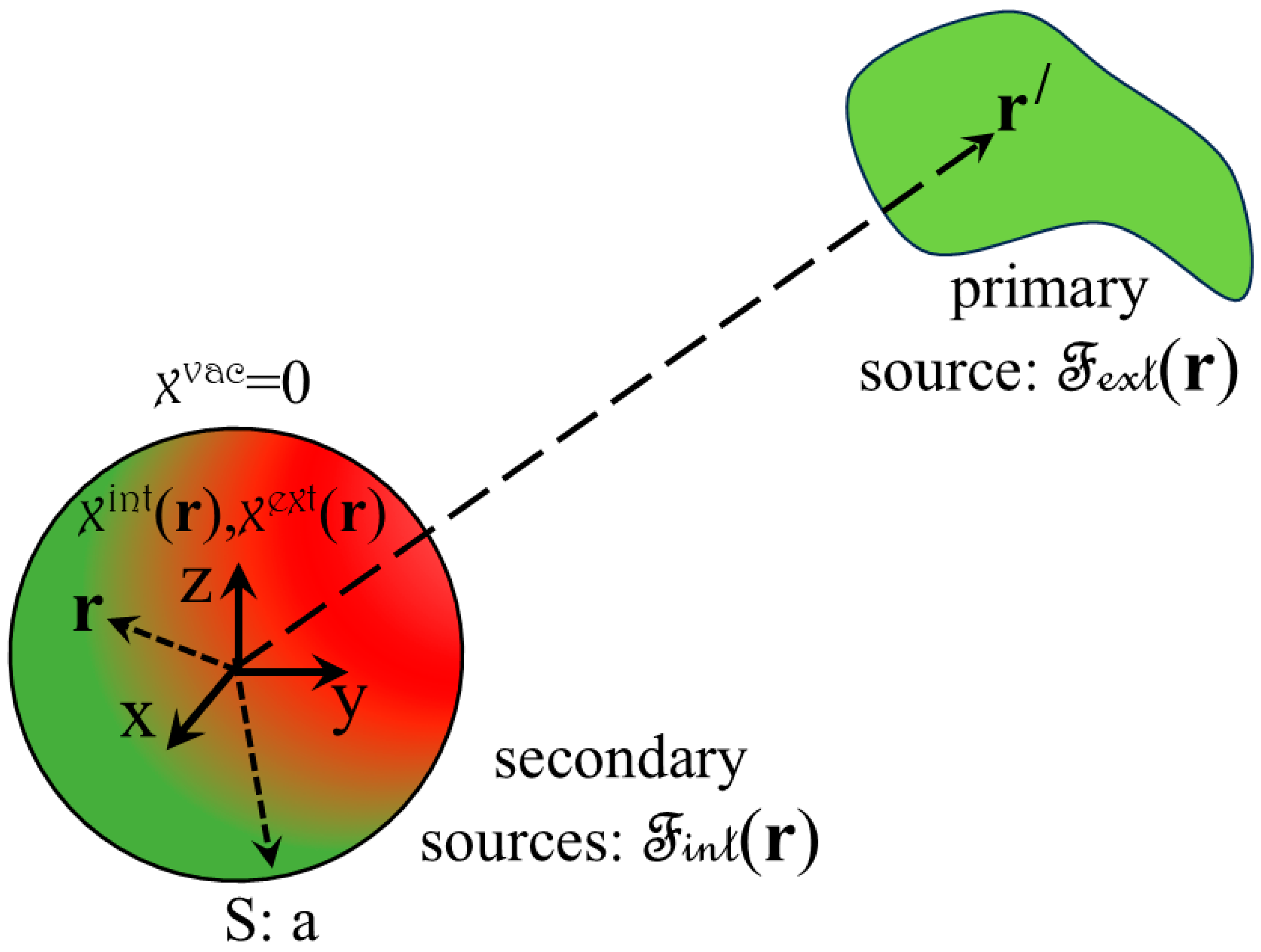
Disclaimer/Publisher’s Note: The statements, opinions and data contained in all publications are solely those of the individual author(s) and contributor(s) and not of MDPI and/or the editor(s). MDPI and/or the editor(s) disclaim responsibility for any injury to people or property resulting from any ideas, methods, instructions or products referred to in the content.

