Grain Knowledge Graph Representation Learning: A New Paradigm for Microstructure-Property Prediction

Abstract

The mesoscopic structure significantly affects the properties of polycrystalline materials. Current artificial-based microstructure-performance analyses are expensive and require rich expert knowledge. Recently, some machine learning models have been used to predict the properties of polycrystalline materials. However, they cannot capture the complex interactive relationship between the grains in the microstructure, which is a crucial factor affecting the material’s macroscopic properties. Here, we propose a grain knowledge graph representation learning method. First, based on the polycrystalline structure, an advanced digital representation of the knowledge graph is constructed, embedding ingenious knowledge while completely restoring the polycrystalline structure. Then, a heterogeneous grain graph attention model (HGGAT) is proposed to realize the effective high-order feature embedding of the microstructure and to mine the relationship between the structure and the material properties. Through benchmarking with other machine learning methods on magnesium alloy datasets, HGGAT consistently demonstrates superior accuracy on different performance labels. The experiment shows the rationality and validity of the grain knowledge graph representation and the feasibility of this work to predict the material’s structural characteristics.

1. Introduction

The material’s crystal structure is of great significance to the research and development of modern advanced metal materials [1,2,3]. Micro-domain grains, texture, and others affect the formability of a part, which is directly related to the material’s mechanical properties [4,5,6,7]. Regarding aerospace materials such as titanium alloys, the texture is carefully controlled during processing to obtain higher corrosion resistance and strength [8]. For auto body parts, magnesium alloys (or aluminum alloys) with excellent strength and ductility can be obtained by adjusting the texture [9,10]. Moreover, the mechanical properties of steel (i.e., tensile strength and formability) are also improved by controlling the grain size [11,12]. It is imperative to understand how the material’s structure affects the material’s performance.

At present, there are two main methods for analyzing the properties of polycrystalline structures: qualitative manual analysis and physical modeling. The methods based on qualitative manual analysis include orientation distribution analysis, inverse pole figure analysis, grain size analysis, etc. Based on this statistical approach, researchers observe specific features through images or statistical functions, thereby establishing a qualitative structure–performance relationship [2,4,5,6,7,9,10,11,12,13]. Another method is to simulate and calculate the structure and properties of materials by establishing physical models, such as Visco-plasitic Self Consistant (VPSC), crystal plasticity finite element method [14,15,16,17,18,19].

With the formation of the “fourth paradigm” of materials science, data-driven methods are increasingly used to explore the relationship between structure and performance [20,21,22,23,24]. Some scholars use the method of statistical descriptors to construct the correlation model between physical characteristics and performance [20,25,26,27,28]. Relevant descriptors are used to represent artificially selected essential features (e.g., grain size and orientation), and then machine learning methods are applied to learn relational functions. Such methods lose the topological information of the microstructure. Another commonly used method is based on image vision [22,29,30,31,32,33]. The scanned image of the organization structure is input into the convolutional neural network (CNN) [34,35]; then, CNN learns the low-dimensional microstructure embedding representation; and finally, the target output is obtained through the fully connected layer [36] or the softmax layer [37]. This type of method guarantees the integrity of the polycrystalline structure (visually) but loses the individual grains’ characteristics and ignores the polycrystalline space’s topological structure. Therefore, the established structure–performance mapping is also biased. Recently, Minyi Dai et al. used Graph Neural Network (GNN) [38,39] to embed the polycrystalline structure [40]. They used nodes to represent grains, edges to represent grain boundaries, and Graph Convolutional Network (GCN) [41,42] to predict the performance of microstructures. This method preserves the topological characteristics of the microstructure through graph embedding. However, the isomorphic graph constructed in this work only expresses the polycrystalline structure’s most straightforward and prominent characteristics. In the actual environment, the polycrystalline structure shows more complex relationships (e.g., different grain boundaries and distribution of similar grains). Moreover, this work uses direct numerical attributes in node descriptions, which is not conducive to network learning [43].

Based on these problems, the following challenges need to be overcome: (1) find a method to effectively digitize the collected microstructure information within the characterization framework, and then, develop a more advanced microstructure “fingerprint” program; (2) design an algorithm that can extract and effectively quantify the representative features (main components) of the microstructure, and then, further establish a rapid, objective, and symmetric structure-performance quantification model.

To solve the above challenges, we propose a digital structured representation method based on a Knowledge Graph (KG) [44,45] and design a heterogeneous grain graph convolutional network, HGGAT. KG can objectively and effectively describe the real objective world, and heterogeneous KG is first used to characterize material grain structure. We provide evidence that KG can realize the effective information digitization of the microstructure. HGGAT can effectively extract the higher-order representative features of the structure and establish the quantitative relationship between the structure and the performance.

2. Materials and Methods

2.1. Dataset

2.1.1. Polycrystal Sample Preparation

This work uses five types of magnesium alloy plates for experiments. The difference in grain orientation and grain size mainly causes changes in their properties. These alloys with normal composition Mg-2Zn, Mg-2Zn-1Li, Mg-2Zn-3Li, Mg-2Zn-1Gd, and AZ31 (Mg-3Zn-1Al) were prepared from Mg (99.9%), Al (99.9%), Zn (99.9%), and Mg-5Li (Wt) (Jiangxi Shida Magnesium Alloy Technology Co., Ltd., location: Ganzhou, Jiangxi, China). The Mg-2Zn alloy charge was heated to 750 °C in an induction furnace (Shanghai Haoyue Electric Furnace Technology Co., Ltd., location: Shanghai, China) protected by Ar gas and kept at 750 °C for 20 min. Then, the liquid alloy was poured into the cylindrical mold with $\phi$95 mm × 480 mm and cooled down in the air. Finally, the ingot was cut to $\phi$82 mm by the machine tool (Jiangsu Siji Machine Tool Co., Ltd., location: Yancheng, Jiangsu, China). The rest of the Mg-2Zn-1Li, Mg-2Zn-3Li, Mg-2Zn-1Gd, AZ31 were produced using the identical process. The chemical compositions are shown in

Table 1. Chemical compositions of the as-cast alloys (wt%).

Alloy	Mg	Zn	Li	Al
Mg-2Zn	Bal	1.99	-	-
Mg-2Zn-1Li	Bal	1.67	1.11	-
Mg-2Zn-3Li	Bal	1.82	3.08	-
Mg-2Zn-1Gd	Bal	1.74	0.97	-
AZ31	Bal	2.98	-	0.99

using the inductively coupled plasma-atomic emission spectroscopy (ICP-AES) ( Analytik Jena AG, location: Jena, Germany). These cylindrical ingots were removed from the surface oxide layer and homogenized at 380 °C for 8 h before extrusion. Afterward, these ingots were extruded at 430 °C with a final thickness of 2 mm.

2.1.2. Dataset Preparation

The microstructure and texture were measured using electron backscattered diffraction (EBSD) (Oxford Instruments, location: Oxford, United Kingdom) on the ED-ND plane in a dual-beam focused ion beam scanning electron microscopy (FIB-SEM, TESCAN AMBER) (TESCAN, location: Brno, Czech). These samples were prepared by grinding on 800#, 1600#, and 3500# SiC sandpapers; then, the electrochemical polishing method for 90–100 s at 20 V, 0.05 A and −15 °C was used to optimize the ED-ND plane further.

The tensile specimens with a gauge length of 12 mm and a width of 6 mm were employed from the extruded samples to measure yield strength (YS) and elongation (EL). Uniaxial tensile tests with a speed of 2 mm/min were performed in the direction of the transverse direction relative to the extruded direction at room temperature.

Based on the above materials, we used the EBSD technology to scan the polycrystalline structure and to obtain nearly 7.03 million scanning point data. After cleaning and denoising the data, we built a knowledge graph of the crystal grains. Finally, the number of grain nodes constructed reached 77,110, the number of attribute nodes formed by the discrete attribute knowledge was 58, and the total number of edges reached 745,784. The model uses the graph as input and the mechanical properties as the corresponding label.

2.2. Representation of the Grain Knowledge Graph

This section constructs the knowledge graph representation [44,46] of the microscopic polycrystalline structure. The polycrystalline microstructure is composed of crystal grains separated by grain boundaries. The grains are located in space with a specific orientation, and the properties and spatial distribution of the crystal grains have an impact on the material’s mechanical properties. Inspired by the Knowledge Graph, we regard the microstructure structure as a huge graph, with the grains in the structure as nodes and the grain boundaries as edges, as shown in Figure 1. Using the methods of texture analysis [47,48] and grain size analysis [49,50] for reference, we discretize the orientation and size of the grains to form easy-to-understand knowledge and embed it in the graph. The discretized orientation categories and size categories are instantiated as attribute nodes in the graph. Based on the idea of object similarity in SimRank [51,52], attribute nodes are connected with corresponding grain nodes to form attribute edges.

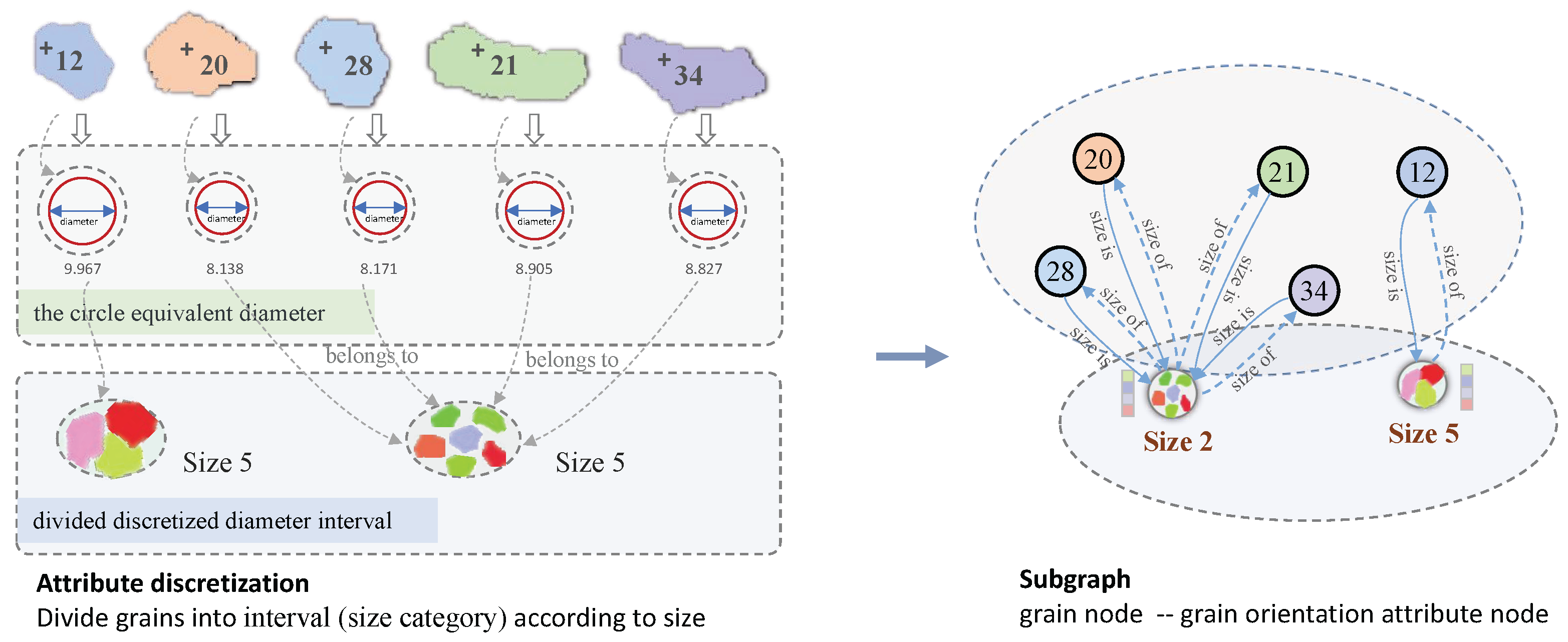
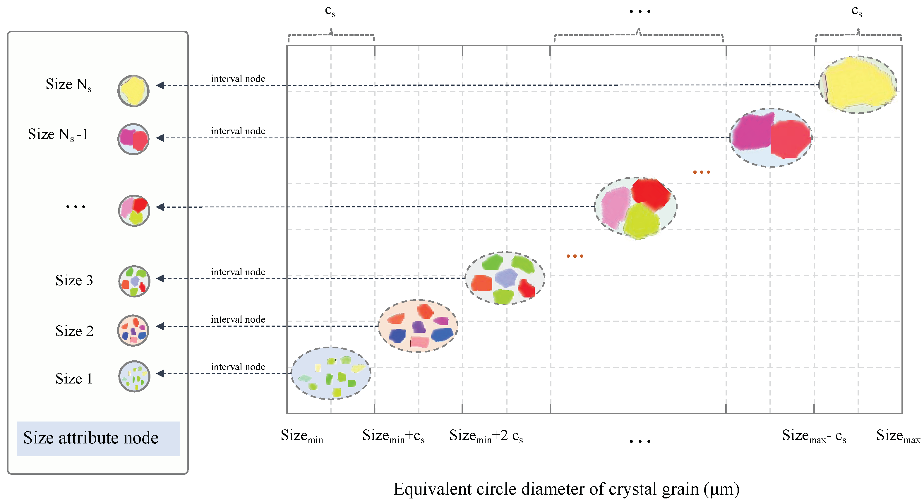
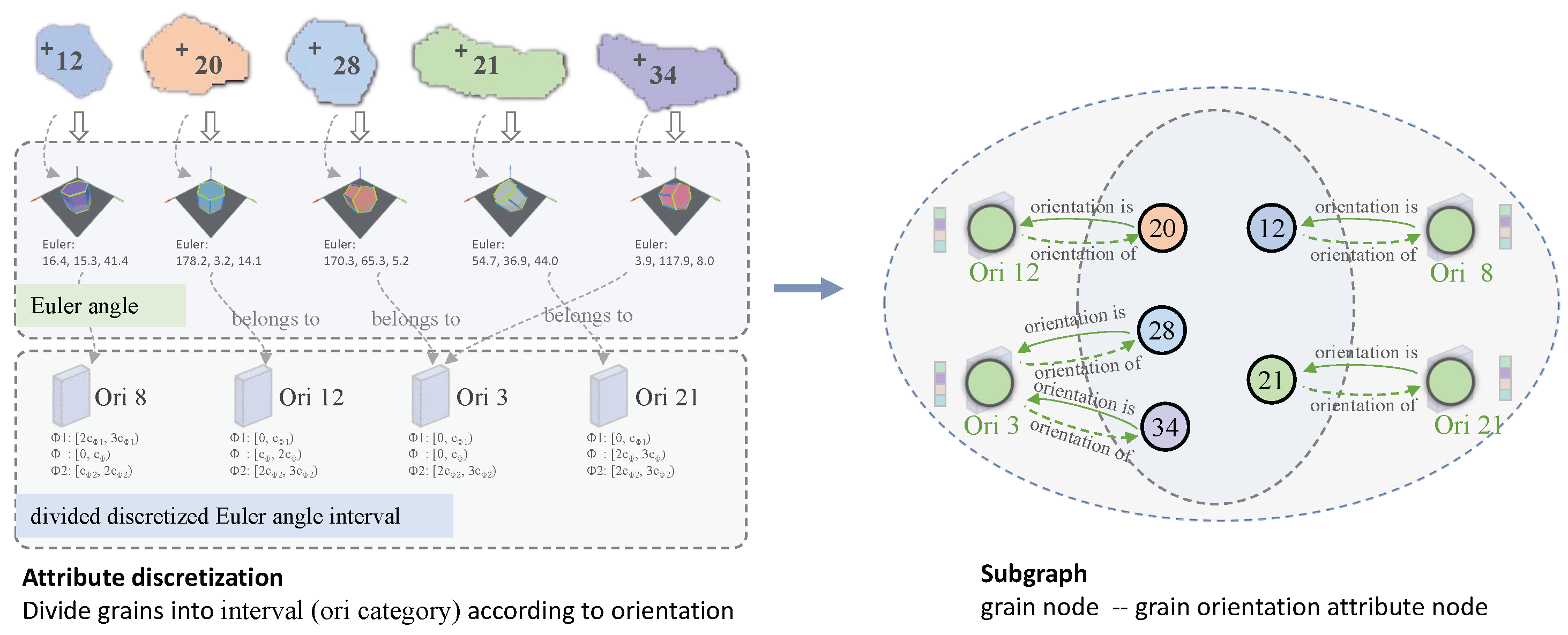
2.2.1. Node Representation

Grain Node Construction. The grain is the central basic unit in the mesoscopic polycrystalline structure we studied, so we extracted it to construct the grain node. Specifically, we use Atex software [53] to give each crystal grain in the microstructure an independent number, which is used to distinguish and identify each crystal grain. Then, we initialize a grain node in the grain knowledge graph for each grain. Figure 2 shows the formation process of the grain node. Grain nodes represent the information and existence of individual grains.

Size Attribute Node Construction. Metal grain size has a decisive influence on its mechanical properties at room temperature and high temperature. In the analysis of metal properties, grain size number analysis is fundamental [49,50]. Therefore, we also embed knowledge of grain size levels in this work. As shown in Figure 3, we divide the crystal grains with the super parameter $c_s$ as the interval length, and each interval represents a kind of grain size. The discrete interval type is more in line with knowledge expression and machine understanding than the original numerical size to describe the grain size.

Equation (1) shows the calculation method of the grain size level. After calculating all of the grain size intervals, we construct the size attribute nodes, which correspond to the interval categories one-to-one. The built size attribute node will be used to reflect the size properties of the grains.

$$L\_S_{node}\hspace{0.17em}=\hspace{0.17em}\lceil (Grain.size-Siz{e}_{min}/c_s\rceil$$

(1)

where $L\_S_{node}$ is the grain size interval category. $Grain.size$ represents the grain diameter, $Siz{e}_{min}$ represents the smallest-scale grain size, $c_s$ denotes the interval length, $\lceil \rceil$ refers to rounding up operation.

Orientation Attribute Node Construction. Similarly, we discretize orientation and build the orientation attribute node. In texture analysis, the orientation distribution of micro-regions is the main observation object. Orientation differentiation appears in the regional distribution. Therefore, establishing discrete intervals of orientation and obtaining statistical distribution information of grain orientation is beneficial to highlighting the characteristics of the organization structure. The grain’s three Euler angles $(\varphi 1,\varphi ,\varphi 2)$ determine its orientation. Figure 4a shows an example of the distribution of grain orientations in a structure. The orientation is three-dimensional data. Therefore, we need to discretize the three-dimensional orientation space, classifying infinite orientation points into finite categories. As shown in Figure 4b, we take $c_{\varphi 1}$, $c_{\varphi }$, and $c_{\varphi 2}$ as the interval division step lengths of $\varphi 1$, $\varphi$, and $\varphi 2$, respectively. Then, the intervals divided by three latitudes constitute a three-dimensional split space. Each divided space is a discrete orientation category. The specific calculation process is shown in Equations (2) and (3), ${\mathit{\varphi }}_{max}$ = $\{\varphi 1_{max},{\varphi }_{max},\varphi 2_{max}\}$, ${\mathit{\varphi }}_{min}$ = $\{\varphi 1_{min},{\varphi }_{min},\varphi 2_{min}\}$ are the largest and smallest grain Euler angles, respectively. According to the length of the three division intervals ${\mathit{c}}_{\varphi }(c_{\varphi 1},c_{\varphi },c_{\varphi 2})$, the Euler angle $\mathit{\varphi }(\varphi 1,\varphi ,\varphi 2)$ are divided into ${\mathit{N}}_{\varphi }$$(N_{\varphi 1},N_{\varphi },N_{\varphi 2})$ equal parts. As a result, a total of $N_o$ three-dimensional subspaces are divided. Equation (4) calculates the subspace number where the crystal grain is located. Finally, we construct the orientation attribute node corresponding to each divided space. Each node represents an orientation category, reflecting the nature of orientation, as shown in Figure 4c.

$$\begin{array}{cc}\hfill c_{\varphi 1}& =(\varphi 1_{max}-\varphi 1_{min})/N_{\varphi 1}\hfill \\ \hfill c_{\varphi }& =({\varphi }_{max}-{\varphi }_{min})/N_{\varphi }\hfill \\ \hfill c_{\varphi 2}& =(\varphi 2_{max}-\varphi 2_{min})/N_{\varphi 2}\hfill \end{array}$$

(2)

$$\begin{array}{c}\hfill N_o=N_{\varphi 1}\times N_{\varphi }\times N_{\varphi 2}\end{array}$$

(3)

$$\begin{array}{cc}\hfill L\_O_{node}\hspace{0.17em}=\hspace{0.17em}\{& \lceil (Grain.\varphi 1-\varphi 1_{min})/c_{\varphi 1}\rceil ,\hfill \\ \hfill & \lceil (Grain.\varphi -{\varphi }_{min})/c_{\varphi }\rceil ,\hfill \\ \hfill & \lceil (Grain.\varphi 2-\varphi 2_{min})/c_{\varphi 2}\rceil \}\hfill \end{array}$$

(4)

where $L\_O_{node}$ refers to the grain orientation subspace number, i.e., the grain orientation category.

2.2.2. Edge Representation

Grain-Grain Edge Construction. The plastic deformation, strength, fracture, brittleness, and other properties of polycrystalline materials are very different from those of single-crystal materials, mainly because the special properties of varying grain boundaries affect the different properties of the alloy. Therefore, a crucial element in the polycrystalline structure is the grain boundary, reflecting the transformation of the atomic arrangement and the interaction between crystal grains. Here, we embed the knowledge information of the grain boundary in the grain knowledge graph by constructing the edges between the grains. First, according to the grain boundaries between the original grains, we build edges between the corresponding grain nodes, corresponding to the grain boundaries. This edge characterizes the interaction and topological structure of the crystal grains. Then, a more specific neighboring interaction rule is established to embed richer structural knowledge. As shown in Equation (5), $\zeta$ is the ratio of the grain boundary length to the total side length. When $\zeta$ is greater than the threshold hyperparameter $\lambda$, the edges between the grains indicate strong, otherwise weak connection, as shown in the Equation (6). The constructed edge (subgraph) is shown in Figure 5.

$$\zeta =boundlength/perimeter$$

(5)

$$Rel\_G\_G\left(\zeta \right)=\left\{\begin{array}{cc}\mathrm{strongly}\mathrm{connect},\hfill & \zeta \ge \lambda \hfill \\ \mathrm{weakly}\mathrm{connect},\hfill & \zeta <\lambda \hfill \end{array}\right.$$

(6)

where $boundlength$ denotes the grain boundary length and $perimeter$ denotes the total side length of the grain. $Rel\_G\_G$ represents the edge type between grains.

Grain-Size Edge Construction. In Section 2.2.1, the size attribute node and the orientation attribute node are constructed. Here, the grain node and the matching attribute node are connected to form a completed grain attribute subgraph. For the size attribute node, we connect it to all matching grain nodes to correlate the size properties of the grains. At the same time, the formed grain size attribute subgraph can reflect the grain size distribution in the microstructure. The specific method is shown in Figure 6, for grains {12, 20, 28, 21, 34}. First, their size levels (categories) {5, 2, 2, 2, 2} are calculated according to Equation (1). Then, the corresponding size attribute nodes are connected to the grain nodes. “size is” and “size of” are the two relationships between the grain node and the size attribute node.

Grain-Orientation Edge Construction. Similarly, we construct the grain orientation attribute subgraph (i.e., the edges between grain nodes and orientation attribute nodes). The orientation attribute node is used to correlate the orientation properties of the grains, and the formed orientation attribute subgraph can also reflect the orientation distribution characteristics of the tissue structure. The specific method is shown in Figure 7. The orientation categories {5, 2, 2, 2, 2} of the grains {12, 20, 28, 21, 34} are calculated by Equation (4), and then, the corresponding orientation attribute nodes are connected to the grain nodes. “ori is” and “ori of” are the two relationships between the grain node and the orientation attribute node.

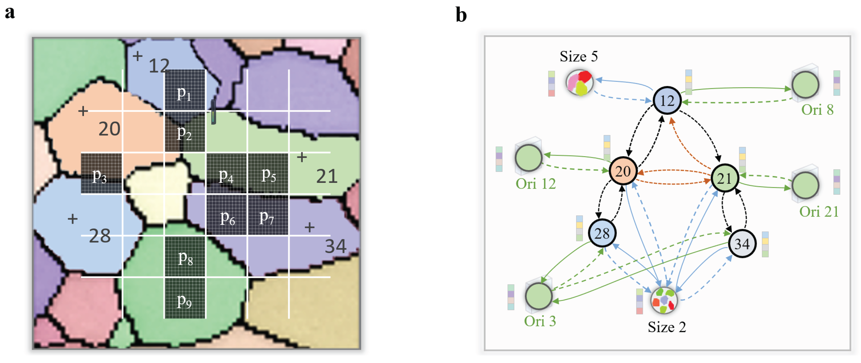
2.2.3. Representation Structure Analysis

Figure 8 shows the original microstructure and the characterization structure constructed in this paper. The proposed structure has two key characteristics: (1) the heterogeneous graph describes the organization more complete and restores the microstructure information; (2) the knowledge graph is easier to understand and calculate using a computer.

The grain structure in Figure 8a is completely embedded in the heterogeneous graph in Figure 8b, and information such as grains and grain boundaries are expressed. Compared with image, the form of a graph is more in line with polycrystalline structure characteristics. When a computer understands an image, it uses pixels as the basic unit to perform statistical calculations. As shown in Figure 8a, ${\mathrm{p}}_2$ contains the parts of grain 12, grain 20, and grain 21, i.e., the area contains the pixels of the three kinds of grains. For computer storage, the pixel storage is continuous, and individual grains are not distinguished. Therefore, in the ${\mathrm{p}}_2$, ${\mathrm{p}}_3$, and ${\mathrm{p}}_4$ regions, there are two-grain boundaries or even three-grain boundaries, and the computer cannot directly and accurately determine and count the grain boundary information.

Moreover, we also added discrete attribute nodes in the graph to enhance knowledge expression. As shown in Figure 8b, the sizes of the grains 20, 21, 28, and 34 are all Size 2. We built a subordination relationship between these grain nodes and the Size 2 node, using similarity transitivity to cluster the nodes with the same attributes. In this way, all nodes with the same attributes are two-hop nodes with each other, and a second-order neighbor relationship is established between the originally uncorrelated or low-correlation nodes. Thus, the computer would pay attention to the cluster information when it understands the graph. The same goes for the orientation attribute node.

2.3. Grain Knowledge Graph Representation Calculation

After completing the representation of the polycrystalline structure, we verify the method’s feasibility through representation calculations. Therefore, we designed a Heterogeneous Grain Graph Attention Model (HGGAT) for the constructed knowledge graph. Through this model, the high-order embedding of the microstructure can be obtained, and the mapping relationship between structure and performance can be established.

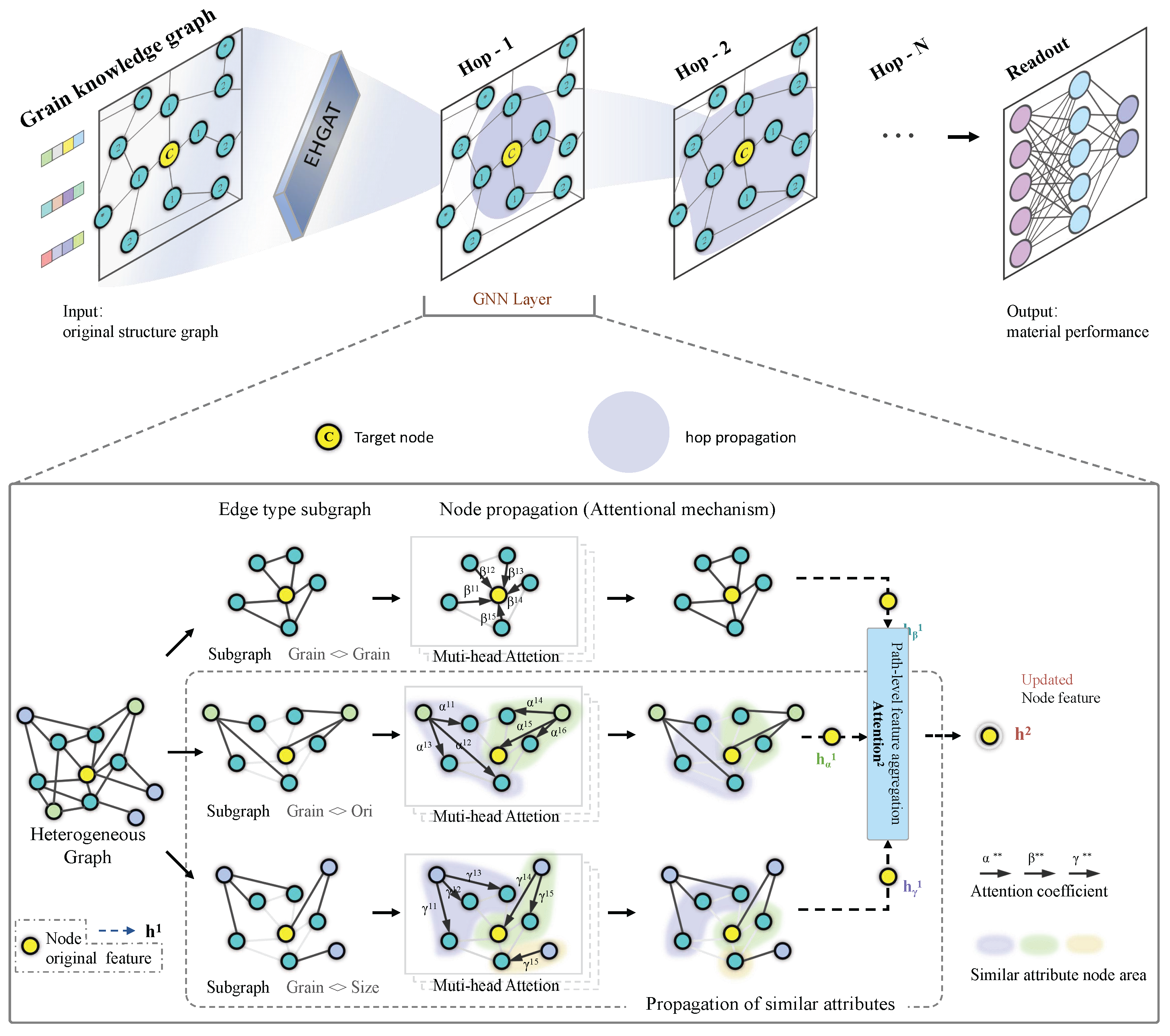
2.3.1. Overview of the HGGAT

As shown in Figure 9, HGGAT is a two-layer heterogeneous graph attention network (GAT) [38,54,55]. First, the input grain graph is divided into a grain isomorphism graph (grain subgraph) and two grain attribute bipartite graphs (attribute subgraphs). When the nodes propagate in the attribute subgraph, the grain nodes connecting the same attribute node absorbs the same attribute characteristics and have a similarity. When the nodes propagate in the grain subgraph, the nodes with similar characteristics are more easily aggregated to obtain a more enhanced feature distribution. The attention mechanism (node-level attention) is used in the subgraph (meta-paths) convolution. After the message passing on all subgraphs (meta-paths), a path-level attention network is used to aggregate the features of the same node on different subgraphs (meta-paths). The attention of the meta-path captures the influencing factors between nodes so that the nodes can focus on more essential features. The optimal combination is obtained by path-level attention when aggregating different path nodes. In addition, the model can learn the complex and rich information in heterogeneous graphs better. Through the message transmission and aggregation of different relationships, the grain nodes in the graph continuously capture the characteristics of more and more nodes around them. Finally, the readout operation extracts the graph-level feature embedding and maps the embedding to the material properties.

2.3.2. The Propagation Process of HGGAT

For each set of data, we used the grain knowledge graph G as input and the material performance Y as a label. The goal of the model is to learn the mapping from graph to performance (i.e., $\Gamma :G\to Y$). The model contains two processes: graph convolution feature extraction and label mapping. Convolution mainly includes two parts: (1) convolution on independent subgraphs; (2) feature fusion of the same nodes on different subgraphs. Equations (7)–(10) show the convolution process in the subgraph. ${\overrightarrow{h}}_i^{k^{\left(\iota \right)}}$ is the initial feature of the k-layer (lower layer) node, $\iota$ represents different paths/edges (subgraph), and $\mathit{W}$ is a learnable weight matrix. First, the lower layer embedding is linearly transformed to form higher-order features ${\overrightarrow{z}}_i^{k^{\left(\iota \right)}}$.

$${\overrightarrow{z}}_i^{k^{\left(\iota \right)}}={\mathit{W}}^{k^{\left(\iota \right)}}·{\overrightarrow{h}}_i^{k^{\left(\iota \right)}}$$

(7)

Then, a paired unnormalized attention score $e_{ij}^{k^{\left(\iota \right)}}$ between two neighbors is calculated using the dot product on the splicing embedding of two adjacent nodes.

$$e_{ij}^{k^{\left(\iota \right)}}=LeakyReLU({\overrightarrow{a}}^{k^{\left(\iota \right)}}·[{\overrightarrow{z}}_i^{k^{\left(\iota \right)}}\Vert {\overrightarrow{z}}_j^{k^{\left(\iota \right)}}])$$

(8)

where $\overrightarrow{a}$ denotes a learnable weight vector, ‖ means concatenation, · represents the dot product, and $LeakyReLU$ is the activation function. Next, the softmax layer is used to normalize the attention score on the incoming edge of each node.

$${\alpha }_{ij}^{k^{\left(\iota \right)}}=Softma{x}_j(e_{ij}^{k^{\left(\iota \right)}})$$

(9)

where j denotes the incoming node. Finally, according to the calculated attention score, the embeddings from neighboring nodes are scaled and aggregated together.

$${\overrightarrow{h}}_i^{{k+1}^{\left(\iota \right)}}=\sigma (\sum _{j\in {N\left(i\right)}^{\left(\iota \right)}}{\alpha }_{ij}^{k^{\left(\iota \right)}}·{\overrightarrow{z}}_i^{k^{\left(\iota \right)}})$$

(10)

where $N\left(i\right)$ represents all neighbors of node i. $h_i^{k+1}$ denotes the $(k+1)$-layer (higher layer) feature embedding of node i. $\sigma$ is an activation function.

After the message passing of all subgraphs (meta-paths), path-level attention is used to aggregate the features of the same node on different subgraphs (meta-paths). ${\beta }_{\left(\iota \right)}^k$ is an important coefficient of meta-path $\iota$. First, the updated node embedding ${\overrightarrow{h}}_i^{{k+1}^{\left(\iota \right)}}$ of each subgraph is non-linearly transformed; then a similarity measurement is achieved with a learnable vector $\overrightarrow{q}$; next, a softmax operation is performed to obtain important coefficients. Finally, the node embeddings on each meta-path are weighted and summed.

$$\begin{array}{cc}\hfill {\beta }_{\left(\iota \right)}^k& =Softmax(\frac{1}{N\left(i\right)}\sum _{\iota \in N\left(i\right)}\overrightarrow{q}·tanh({\mathit{W}}^k·{\overrightarrow{h}}_i^{{k+1}^{\left(\iota \right)}}+\overrightarrow{b}))\hfill \\ \hfill {\overrightarrow{h}}_i^{k+1}& =\sum _{\iota =1}^p{\beta }_{\left(\iota \right)}^k·{\overrightarrow{h}}_i^{{k+1}^{\left(\iota \right)}}\hfill \end{array}$$

(11)

where $\overrightarrow{b}$ represents the bias vector, $tanh$ denotes the activation function, p refers to the number of edge types (the number of subgraphs), and ${\overrightarrow{h}}_i^{k+1}$ is the final updated node embedding.

After completing multiple graph convolutions, highly abstract node embedding is obtained. Then, we use a readout operation (average pooling) to obtain the graph-level node representation $\overrightarrow{H}$ and to map it to the material properties $Y^{\prime }$ with fully connected layers [56] (FC).

$$\begin{array}{cc}\hfill \overrightarrow{H}& =\frac{1}{N\left(g\right)}\sum _{i\in N\left(g\right)}{\overrightarrow{h}}_i^{k+1}\hfill \\ \hfill Y^{\prime }& =ReLU(\mathit{a}·\overrightarrow{H}+\overrightarrow{b^{\prime }})\hfill \end{array}$$

(12)

where $N\left(g\right)$ denotes all grain nodes, $\overrightarrow{H}$ represents the graph-level embedding, $ReLU$ is activation function, $\mathit{a}$ is a learnable weight matrix, $\overrightarrow{b^{\prime }}$ is a bias vector, and $Y^{\prime }$ is the predicted performances (mechanical properties).

After completing the forward propagation to obtain the prediction result, the mean square error is used to calculate the L2 loss (error between $Y^{\prime }$ and Y). Through gradient descent to reduce loss, the model is continuously optimized.

$$L2=\frac{1}{n}\sum _{m=1}^n{(Y_m^{\prime }-Y_m)}^2$$

(13)

3. Results

3.1. Experiment Settings

To evaluate the performance of HGGAT and to prove that the paper method is superior to well-known machine learning methods, we designed a representative comparative experiment. We selected the most popular and representative machine learning algorithms: Ridge, Support Vector Regression (SVR), K-Nearest Neighbor (KNN), Random Forest (RF), and Multilayer Perceptron (MLP). For the machine learning algorithms, the raw statistical data are used as input, i.e., the inputs are the average, maximum, and minimum grain size and the average, maximum, and minimum orientation (Euler angles); for HGGAT, the grain knowledge graph is used as input. Their outputs are the mechanical properties (yield strength, ultimate tensile strength, and elongation). To further highlight the superiority of our graph of adding attribute nodes, our method is also compared with the graph with grain size and orientation simply as scalar grain node attributes. In this isomorphic graph, the grain size and orientation are directly as node attributes of grain nodes, which means that there is only one type of node (grain node) in the graph. Its performance evaluation is shown in the Grain Graph Attention Model (GGAT) row of

Table 2. Multi-label learning model performance of yield strength (YS), ultimate tensile strength (UTS), and elongation (EL). ↑(↓) means that, the higher (lower), the better (worse).

Model	MSE ↓	MAE ↓	EV ↑	${\mathbf{R}}^2$↑
Ridge	0.139	0.299	0.850	0.836
SVR	0.176	0.351	0.796	0.792
KNN	0.160	0.336	0.834	0.810
RF	0.157	0.250	0.841	0.802
MLP	0.153	0.305	0.844	0.819
GGAT	0.116	0.234	0.873	0.865
HGGAT(Our)	0.051	0.164	0.943	0.941

. In all experiments, 80% of the data is randomly selected for training and 20% is selected for testing; 10-fold cross-validation is applied in the training process; Mean Squared Error (MAE), Root Mean Squard Error (MSE), Explained Variance (EV), and R Squared (${\mathrm{R}}^2$) are used to evaluate the performance of each method in the results.

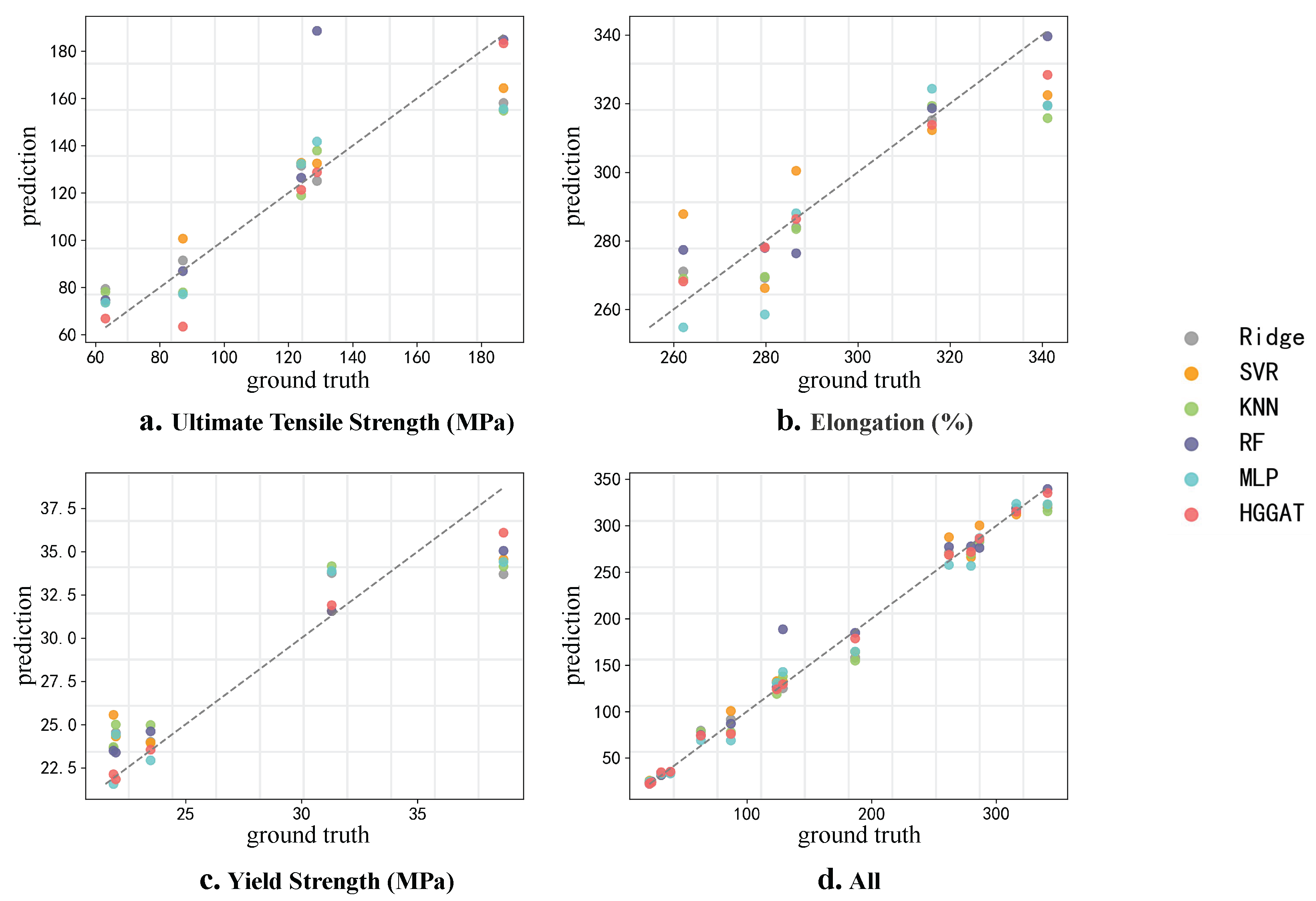
3.2. Prediction Results

The experimental results show that HGGAT shows better performance than other methods in general. For material performance optimization problems, improving a performance often comes at the cost of a decrease in the opposite performance. Therefore, it is difficult to balance various performances and to obtain a better result. With the help of artificial intelligence technology, the model constructed in this paper can predict multiple performances simultaneously. Table 2 shows the model performance for the simultaneous fitting of three attributes (yield strength, ultimate tensile strength, and elongation),i.e., model performance under multi-label learning predictions. Obviously, our HGGAT model has achieved the best in all indicators and even achieved a very impressive ${\mathrm{R}}^2$ value of 0.941, which is significantly better than other methods. Those machine learning methods can learn the statistical characteristics of grains and grain boundaries and can capture the impact of different characteristics on performance. However, they can neither capture the effects of different granularities nor ignore the high-order relationship features (i.e., interaction between grains and topological structure of organization), so their performance is relatively poor. Even if an optimal parameter search is used, their performance is still far behind HGGAT. HGGAT uses graphs comparing grain size and orientation, presented as simply scalar grain node attributes, as the input and is consistent with HGGAT in the main structure. In terms of model performance, this graph learning method exhibits better performance than traditional machine learning methods, but it is slightly worse than our method.

In addition to multi-attribute (multi-label) learning and prediction, HGGAT also stands out in single-attribute (single-label) learning and prediction. We use a single attribute as a label to train all contrast models. As shown in Figure 10, the model fitting results for different prediction targets are arranged in each row. In the YS prediction, HGGAT achieved the highest ${\mathrm{R}}^2$ value of 0.93; in the UTS prediction, HGGAT achieved the highest ${\mathrm{R}}^2$ value of 0.94; and in the EL prediction, HGGAT achieved the highest ${\mathrm{R}}^2$ value of 0.93. It proves that the scattered points of HGGAT are closest to the fitted line, indicating that the prediction accuracy of HGGAT is the highest.

4. Discussion and Conclusions

All materials have specific structural dimensions and characteristics that determine their performance. For polycrystalline materials, the nature of the grain structure is a critical internal factor that affects its mechanical properties. Based on the fourth paradigm of data-driven materials research, this paper reports a novel representation method based on knowledge graphs and an artificial intelligence model, which realizes the scientific grain structure digital representation and calculation of the structure–performance relationship.

As a digital representation method, the grain knowledge graph can completely restore the original polycrystalline structure information. It uses nodes to describe the grains in the material microstructure and directly stores grain boundary information through different edges. Therefore, it is worth mentioning that the grain knowledge graph stores the grains’ spatial topological structure while retaining the properties of the original grains. Second, on the basic graph, discrete descriptions of critical attributes are added further. We divide grains according to grain size, orientation, and boundary characteristics and construct subgraphs of grain nodes. We also discrete attribute nodes through expert knowledge. Discrete feature injection into the graph makes the non-linear feature better represent the knowledge level expression.

Based on this digital representation, this paper proposes a targeted heterogeneous grain graph network model HGGAT. From a technical point of view, HGGAT has some advantages. First, unlike other methods, HGGAT uses features, knowledge, and graphical structure to ensure that the polycrystalline structure’s original and critical information is not lost. Second, HGGAT uses the representation learning method to obtain the high-level feature embedding of the polycrystalline structure and then implements the structure-to-performance supervised learning, which is preferable to directly mapping the original features to the label. Third, HGGAT uses a two-layer attention method to disseminate feature information under the same path non-linearly and then to aggregate the messages of all paths. It captures the complex structure by considering the semantic relations of different classes to improve the embedding performance of the model.

Despite the successful results of this work, there are still some areas that can be improved. First, this work is only applicable to ordinary single-phase polycrystalline materials. For other structures such as multiphase and internal twins, additional knowledge representation is needed to improve the scientific accuracy of graph construction. Second, as an artificial intelligence model, although HGGAT shows its powerful data analysis capabilities, it also shows some limitations, including the black-box nature of the AI model. These can be solved using a parameter control and feature analysis, such as graph message transmission control and feature visualization analysis. Finally, with the rapid development of the AI field, the graph construction and graph networks are constantly iterating and updating. Future work will focus on these issues.We will iterate and optimize it in future work.

References

1. Oganov, A.R.; Pickard, C.J.; Zhu, Q.; Needs, R.J. Structure prediction drives materials discovery. Nat. Rev. Mater. 2019, 4, 331–348. [Google Scholar] [CrossRef]
2. Rekha, S.; Raja, V.B. Review on Microstructure Analysis of Metals and Alloys Using Image Analysis Techniques. IOP Conf. Ser. Mater. Sci. Eng. 2017, 197, 012010. [Google Scholar] [CrossRef] [Green Version]
3. Jain, A.; Ong, S.P.; Hautier, G.; Chen, W.; Persson, K.A. Commentary: The Materials Project: A materials genome approach to accelerating materials innovation. APL Mater. 2013, 1, 011002. [Google Scholar] [CrossRef] [Green Version]
4. Li, X.; Lu, L.; Li, J.; Zhang, X.; Gao, H. Mechanical properties and deformation mechanisms of gradient nanostructured metals and alloys. Nat. Rev. Mater. 2020, 5, 706–723. [Google Scholar] [CrossRef]
5. Liu, R.; Tian, Y.; Zhang, Z.; An, X.; Zhang, P.; Zhang, Z. Exceptional high fatigue strength in Cu-15at.% Al alloy with moderate grain size. Sci. Rep. 2016, 6, 27433. [Google Scholar] [CrossRef] [Green Version]
6. Chai, Y.; Jiang, B.; Song, J.; Wang, Q.; He, J.; Zhao, J.; Huang, G.; Jiang, Z.; Pan, F. Role of Al content on the microstructure, texture and mechanical properties of Mg-3.5 Ca based alloys. Mater. Sci. Eng. A 2018, 730, 303–316. [Google Scholar] [CrossRef]
7. He, J.; Mao, Y.; Fu, Y.; Jiang, B.; Xiong, K.; Zhang, S.; Pan, F. Improving the room-temperature formability of Mg-3Al-1Zn alloy sheet by introducing an orthogonal four-peak texture. J. Alloys Compd. 2019, 797, 443–455. [Google Scholar] [CrossRef]
8. Kang, L.; Yang, C. A review on high-strength titanium alloys: Microstructure, strengthening, and properties. Adv. Eng. Mater. 2019, 21, 1801359. [Google Scholar] [CrossRef]
9. Ahmad, R.; Yin, B.; Wu, Z.; Curtin, W. Designing high ductility in magnesium alloys. Acta Mater. 2019, 172, 161–184. [Google Scholar] [CrossRef]
10. Joost, W.J.; Krajewski, P.E. Towards magnesium alloys for high-volume automotive applications. Scr. Mater. 2017, 128, 107–112. [Google Scholar] [CrossRef]
11. Shao, C.; Zhang, P.; Zhu, Y.; Zhang, Z.; Pang, J.; Zhang, Z. Improvement of low-cycle fatigue resistance in TWIP steel by regulating the grain size and distribution. Acta Mater. 2017, 134, 128–142. [Google Scholar] [CrossRef]
12. Białobrzeska, B.; Konat, Ł.; Jasiński, R. The influence of austenite grain size on the mechanical properties of low-alloy steel with boron. Metals 2017, 7, 26. [Google Scholar] [CrossRef] [Green Version]
13. Carneiro, Í.; Simões, S. Recent advances in EBSD characterization of metals. Metals 2020, 10, 1097. [Google Scholar] [CrossRef]
14. Alian, A.; Meguid, S. Hybrid molecular dynamics–finite element simulations of the elastic behavior of polycrystalline graphene. Int. J. Mech. Mater. Des. 2018, 14, 551–563. [Google Scholar] [CrossRef]
15. Knezevic, M.; Beyerlein, I.J. Multiscale modeling of microstructure-property relationships of polycrystalline metals during thermo-mechanical deformation. Adv. Eng. Mater. 2018, 20, 1700956. [Google Scholar] [CrossRef]
16. Smith, B.; Shih, D.; McDowell, D. Cyclic plasticity experiments and polycrystal plasticity modeling of three distinct Ti alloy microstructures. Int. J. Plast. 2018, 101, 1–23. [Google Scholar] [CrossRef]
17. Wang, Z.; Zhang, J.; Xu, Z.; Zhang, J.; ul Hassan, H.; Li, G.; Zhang, H.; Hartmaier, A.; Fang, F.; Yan, Y.; et al. Crystal plasticity finite element modeling and simulation of diamond cutting of polycrystalline copper. J. Manuf. Process. 2019, 38, 187–195. [Google Scholar] [CrossRef]
18. Sharma, B.B.; Parashar, A. A review on thermo-mechanical properties of bi-crystalline and polycrystalline 2D nanomaterials. Crit. Rev. Solid State Mater. Sci. 2020, 45, 134–170. [Google Scholar] [CrossRef]
19. Sahoo, S.K.; Dhinwal, S.S.; Vu, V.Q.; Toth, L.S. A new macroscopic strain hardening function based on microscale crystal plasticity and its application in polycrystal modeling. Mater. Sci. Eng. A 2021, 823, 141634. [Google Scholar] [CrossRef]
20. Hart, G.L.; Mueller, T.; Toher, C.; Curtarolo, S. Machine learning for alloys. Nat. Rev. Mater. 2021, 6, 730–755. [Google Scholar] [CrossRef]
21. Zhou, Q.; Lu, S.; Wu, Y.; Wang, J. Property-Oriented Material Design Based on a Data-Driven Machine Learning Technique. J. Phys. Chem. Lett. 2020, 11, 3920–3927. [Google Scholar] [CrossRef] [PubMed]
22. Kondo, R.; Yamakawa, S.; Masuoka, Y.; Tajima, S.; Asahi, R. Microstructure recognition using convolutional neural networks for prediction of ionic conductivity in ceramics. Acta Mater. 2017, 141, 29–38. [Google Scholar] [CrossRef]
23. Wang, Z.L.; Adachi, Y. Property prediction and properties-to-microstructure inverse analysis of steels by a machine-learning approach. Mater. Sci. Eng. A 2019, 744, 661–670. [Google Scholar] [CrossRef]
24. Pokuri, B.S.S.; Ghosal, S.; Kokate, A.; Sarkar, S.; Ganapathysubramanian, B. Interpretable deep learning for guided microstructure-property explorations in photovoltaics. NPJ Comput. Mater. 2019, 5, 95. [Google Scholar] [CrossRef] [Green Version]
25. Khosravani, A.; Cecen, A.; Kalidindi, S.R. Development of high throughput assays for establishing process-structure-property linkages in multiphase polycrystalline metals: Application to dual-phase steels. Acta Mater. 2017, 123, 55–69. [Google Scholar] [CrossRef] [Green Version]
26. Yabansu, Y.C.; Patel, D.K.; Kalidindi, S.R. Calibrated localization relationships for elastic response of polycrystalline aggregates. Acta Mater. 2014, 81, 151–160. [Google Scholar] [CrossRef]
27. Yabansu, Y.C.; Kalidindi, S.R. Representation and calibration of elastic localization kernels for a broad class of cubic polycrystals. Acta Mater. 2015, 94, 26–35. [Google Scholar] [CrossRef] [Green Version]
28. Latypov, M.I.; Kühbach, M.; Beyerlein, I.J.; Stinville, J.C.; Toth, L.S.; Pollock, T.M.; Kalidindi, S.R. Application of chord length distributions and principal component analysis for quantification and representation of diverse polycrystalline microstructures. Mater. Charact. 2018, 145, 671–685. [Google Scholar] [CrossRef]
29. Cang, R.; Li, H.; Yao, H.; Jiao, Y.; Ren, Y. Improving direct physical properties prediction of heterogeneous materials from imaging data via convolutional neural network and a morphology-aware generative model. Comput. Mater. Sci. 2018, 150, 212–221. [Google Scholar] [CrossRef] [Green Version]
30. Rong, Q.; Wei, H.; Huang, X.; Bao, H. Predicting the effective thermal conductivity of composites from cross sections images using deep learning methods. Compos. Sci. Technol. 2019, 184, 107861. [Google Scholar] [CrossRef]
31. Chan, H.; Cherukara, M.; Loeffler, T.D.; Narayanan, B.; Sankaranarayanan, S.K. Machine learning enabled autonomous microstructural characterization in 3D samples. NPJ Comput. Mater. 2020, 6, 1. [Google Scholar] [CrossRef]
32. Herriott, C.; Spear, A.D. Predicting microstructure-dependent mechanical properties in additively manufactured metals with machine-and deep-learning methods. Comput. Mater. Sci. 2020, 175, 109599. [Google Scholar] [CrossRef]
33. Yang, C.; Kim, Y.; Ryu, S.; Gu, G.X. Prediction of composite microstructure stress-strain curves using convolutional neural networks. Mater. Des. 2020, 189, 108509. [Google Scholar] [CrossRef]
34. Albawi, S.; Mohammed, T.A.; Al-Zawi, S. Understanding of a convolutional neural network. In Proceedings of the 2017 International Conference on Engineering and Technology (ICET), Antalya, Turkey, 21–24 August 2017; pp. 1–6. [Google Scholar]
35. Sateesan, A.; Sinha, S.; Smitha, K.; Vinod, A. A Survey of Algorithmic and Hardware Optimization Techniques for Vision Convolutional Neural Networks on FPGAs. Neural Process. Lett. 2021, 53, 2331–2377. [Google Scholar] [CrossRef]
36. Sainath, T.N.; Vinyals, O.; Senior, A.; Sak, H. Convolutional, long short-term memory, fully connected deep neural networks. In Proceedings of the 2015 IEEE International Conference on Acoustics, Speech and Signal Processing (ICASSP), Brisbane, Australia, 19–24 April 2015; pp. 4580–4584. [Google Scholar]
37. Yuan, B. Efficient hardware architecture of softmax layer in deep neural network. In Proceedings of the 2016 29th IEEE International System-on-Chip Conference (SOCC), Seattle, WA, USA, 6–9 September 2016; pp. 323–326. [Google Scholar]
38. Zhou, J.; Cui, G.; Hu, S.; Zhang, Z.; Yang, C.; Liu, Z.; Wang, L.; Li, C.; Sun, M. Graph neural networks: A review of methods and applications. AI Open 2020, 1, 57–81. [Google Scholar] [CrossRef]
39. Wu, Z.; Pan, S.; Chen, F.; Long, G.; Zhang, C.; Philip, S.Y. A comprehensive survey on graph neural networks. IEEE Trans. Neural Netw. Learn. Syst. 2020, 32, 4–24. [Google Scholar] [CrossRef] [Green Version]
40. Dai, M.; Demirel, M.F.; Liang, Y.; Hu, J.M. Graph neural networks for an accurate and interpretable prediction of the properties of polycrystalline materials. NPJ Comput. Mater. 2021, 7, 103. [Google Scholar] [CrossRef]
41. Zhang, S.; Tong, H.; Xu, J.; Maciejewski, R. Graph convolutional networks: Algorithms, applications and open challenges. In International Conference on Computational Social Networks; Springer: Berlin/Heidelberg, Germany, 2018; pp. 79–91. [Google Scholar]
42. Zhang, S.; Tong, H.; Xu, J.; Maciejewski, R. Graph convolutional networks: A comprehensive review. Comput. Soc. Netw. 2019, 6, 11. [Google Scholar] [CrossRef] [Green Version]
43. Liu, H.; Hussain, F.; Tan, C.L.; Dash, M. Discretization: An enabling technique. Data Min. Knowl. Discov. 2002, 6, 393–423. [Google Scholar] [CrossRef]
44. Wang, Q.; Mao, Z.; Wang, B.; Guo, L. Knowledge graph embedding: A survey of approaches and applications. IEEE Trans. Knowl. Data Eng. 2017, 29, 2724–2743. [Google Scholar] [CrossRef]
45. Ji, S.; Pan, S.; Cambria, E.; Marttinen, P.; Philip, S.Y. A survey on knowledge graphs: Representation, acquisition, and applications. arXiv 2021, arXiv:2002.00388. [Google Scholar] [CrossRef]
46. Hamilton, W.L. Graph representation learning. Synth. Lect. Artifical Intell. Mach. Learn. 2020, 14, 1–159. [Google Scholar] [CrossRef]
47. Trang, T.; Zhang, J.; Kim, J.; Zargaran, A.; Hwang, J.; Suh, B.C.; Kim, N. Designing a magnesium alloy with high strength and high formability. Nat. Commun. 2018, 9, 2522. [Google Scholar] [CrossRef]
48. Zhang, J.; Tan, T. Brief review of invariant texture analysis methods. Pattern Recognit. 2002, 35, 735–747. [Google Scholar] [CrossRef] [Green Version]
49. Wang, N.; Wang, Z.; Aust, K.; Erb, U. Effect of grain size on mechanical properties of nanocrystalline materials. Acta Metall. Mater. 1995, 43, 519–528. [Google Scholar] [CrossRef]
50. Wang, X.; Shi, T.; Jiang, Z.; Chen, W.; Guo, M.; Zhang, J.; Zhuang, L.; Wang, Y. Relationship among grain size, texture and mechanical properties of aluminums with different particle distributions. Mater. Sci. Eng. A 2019, 753, 122–134. [Google Scholar] [CrossRef]
51. Jeh, G.; Widom, J. Simrank: A measure of structural-context similarity. In Proceedings of the Eighth ACM SIGKDD International Conference on Knowledge Discovery and Data Mining, Edmonton, AB, Canada, 23–26 July 2002; pp. 538–543. [Google Scholar]
52. Yu, W.; Lin, X.; Zhang, W.; Pei, J.; McCann, J.A. SimRank*: Effective and scalable pairwise similarity search based on graph topology. VLDB J. 2019, 28, 401–426. [Google Scholar] [CrossRef] [Green Version]
53. Beausir, B.; Fundenberger, J.J. Analysis Tools for Electron and X-ray Diffraction; Université de Lorraine: Mace, France, 2017. [Google Scholar]
54. Veličković, P.; Cucurull, G.; Casanova, A.; Romero, A.; Lio, P.; Bengio, Y. Graph attention networks. arXiv 2017, arXiv:1710.10903. [Google Scholar]
55. Wang, X.; Ji, H.; Shi, C.; Wang, B.; Ye, Y.; Cui, P.; Yu, P.S. Heterogeneous graph attention network. In Proceedings of the World Wide Web Conference, San Francisco, CA, USA, 13–17 May 2019; pp. 2022–2032. [Google Scholar]
56. Gurney, K. An Introduction to Neural Networks; CRC Press: Boca Raton, FL, USA, 2018. [Google Scholar]
Figure 1. Grain knowledge graph. Each node in the figure represents a crystal grain in the microstructure, and the edges between nodes represent the grain boundaries between the original crystal grains.
Crystals 12 00280 g001
Figure 2. Grain node construction process. Each grain in the IPF map corresponds to each grain node in the graph. Each node stores the features of the grain.
Crystals 12 00280 g002
Figure 3. Grain size discretization and size attribute node construction. S i z e m a x ( S i z e m i n ) denotes the largest-scale grain size (the smallest-scale grain size). According to the interval length c s , the grains are divided into each interval. There are N s intervals in total, N s = ( S i z e m a x S i z e m i n ) / c s . For each interval, the corresponding node on the left is constructed.
Crystals 12 00280 g003
Figure 4. Grain orientation discretization and orientation attribute node construction. (a) Simulated Euler angle data distribution. Each orientation is determined by three Euler points. (b) The three-dimensional orientation space is discretized, and each orientation point can be divided into a discrete three-dimensional space. (c) For each discrete three-dimensional space, the corresponding orientation attribute node is constructed.
Crystals 12 00280 g004
Figure 5. Grain-grain edge construction. According to the connection relationship of the crystal grains (i.e., the grain boundary), the edges between the grain nodes are constructed.
Crystals 12 00280 g005
Figure 6. Grain-size edge construction. First, the corresponding size categories of grains are calculated, and then, the corresponding size category nodes (size attribute nodes) are connected to the grain nodes. In this way, the grain node and the corresponding size attribute node constitute a subordination relationship.
Crystals 12 00280 g006
Figure 7. Grain-orientation edge construction. First, the grains are classified into corresponding orientation categories, and then, the corresponding orientation category nodes (orientation attribute nodes) are connected to the grain nodes. In this way, the grain node and the orientation attribute node constitute a subordination relationship.
Crystals 12 00280 g007
Figure 8. Representation structure comparison. (a) The image storage structure. (b) The grain knowledge graph storage structure.
Crystals 12 00280 g008
Figure 9. Grain graph convolutional prediction model.
Crystals 12 00280 g009
Figure 10. Fitting result. “ Ultimate Tensile Strength” means that UTS is used as the label during training and testing; “Elongation” means that EL is used as the label during training and testing; “Yield Strength” means that YS is used as the label during training and testing; “All” means that UTS, EL, and YS are used together as the label of the data in the experiment, i.e., multi-label learning and prediction task.
Crystals 12 00280 g010