The Freedericksz Transition in a Spatially Varying Magnetic Field

Abstract

Much is known about the Freedericksz transition induced by uniform electric and magnetic fields in nematic liquid crystals. In this work, we are interested in the effects of a spatially varying field on the transition. Specifically, we study the director configuration in a homeotropic nematic cell in a spatially varying magnetic field with cylindrical symmetry. The experiment is conducted with a ring magnet which provides a radial magnetic field with magnitude monotonically decreasing to zero at the center. The nematic cell is positioned in the central plane of the ring, with the cell normal parallel to the ring normal. Interference patterns of the nematic cell between crossed polarizers were observed. The director configuration in the nematic cell is modeled with Frank–Oseen theory, and the computed interference pattern from the simulated director field are compared with experiment. We conclude that if the magnetic field strength varies with position in the plane of the cell, there is no Freedericksz transition.

1. Introduction

Nematic liquid crystals are anisotropic fluids whose constituent particles prefer to align, for reasons of energy and/or entropy, with their symmetry axes parallel. This direction is typically designated by a unit vector $\widehat{\mathbf{n}}$, the nematic director. In the absence of interactions with surfaces or external fields, there is no preferred direction for $\widehat{\mathbf{n}}$; all directions are equally likely. In 1913, Charles Mauguin showed that the nematic director can be aligned by surfaces as well as by a magnetic field [1,2] and in 1927, Vsevolod Freedericksz showed that the nematic director can be aligned by an electric field [3]. If both surface and field alignment interactions are present with different preferred directions, then a competition occurs; as the applied field magnitude is increased, a transition occurs from the surface dominated alignment to the field dominated alignment. This transition is the Freedericksz transition.

One classical example of the Freedericksz transition occurs in a cell with parallel plates with strong homeotropic alignment; i.e., where the surface alignment is such that the director $\widehat{\mathbf{n}}$ is fixed parallel to the surface normal. If a magnetic field $\mathbf{H}$ is applied parallel to the plates, and if the symmetry axes of the molecules prefer to align with the magnetic field in the absence of surface interactions, there will be a competition between the surface anchoring and magnetic field alignment effects. If the field $\mathbf{H}$ is sufficiently strong, the director will change its direction and deviate from the surface normal to align with the field. To do this, it must overcome the Frank [4] elastic energy associated with the spatial variation of the director. The competition between the elastic energy and the interaction energy of the liquid crystal with the field leads to the Freedericksz transition. The generalized Freedericksz transition in cylindrical geometry has been considered in [5].

The dimensionless Landau free energy density of the system can be written in terms of the deviation angle ${\theta }_0$, measured from the surface normal, in the middle of the cell, to leading order, as [6,7],

$$\mathcal{F}=\frac{1}{2}{\theta }_0^2(1-\frac{H^2}{H_c^2})+\frac{1}{8}\frac{H^2}{H_c^2}{\theta }_0^4,$$

(1)

where $H_c$, representing both elastic and magnetic contributions, is the critical magnetic field. Minimizing the free energy with respect to ${\theta }_0$ gives

$${\theta }_0=0,$$

(2)

and

$${\theta }_0=\pm \sqrt{2(1-\frac{H_c^2}{H^2})},$$

(3)

as shown in Figure 1, where we only show the positive branch of the solution.

For $H<H_c$, the only solution is ${\theta }_0=0$; that is to say, $\widehat{\mathbf{H}}·\widehat{\mathbf{n}}=0$ for all $H<H_c$. As the field is increased, at $H=H_c$ a second solution with ${\theta }_0\ne 0$ appears, and for $H>H_c$, ${\theta }_0$ rapidly increases with H and the solution minimizes the free energy. The transition is second order, in accordance with the Landau theory of second order phase transitions [8]. The classical Freedericksz transition, as described above, has received considerable attention. Since it relates elastic properties of liquid crystals to susceptibilities to applied fields, it has been widely used to probe the properties of nematics.

It is interesting to ask what happens if the magnetic field H is not uniform. If H were to vary linearly with position x, ${\theta }_0$ might be expected to depend on position as it does on the field H in Figure 1. However, this would result in a large elastic energy cost due to the rapid variation of ${\theta }_0$ with position.

The work reported here was carried out to answer this question, to find out what happens in the Freedericksz transition when the field driving the transition is not uniform, but varies in space. The details of this work are given below.

2. Experiment

The experiment consisted of optical interferometric measurements on a homeotropically aligned nematic liquid crystal in a planar circular cell placed in a radial magnetic field. The magnitude of the field increased monotonically from zero at the center to a maximum value at the cell perimeter. This geometry provides a well characterized spatially varying field with high symmetry, allowing study of the response of the nematic liquid crystal to the spatially varying magnetic field. Details of the experiment are provided below.

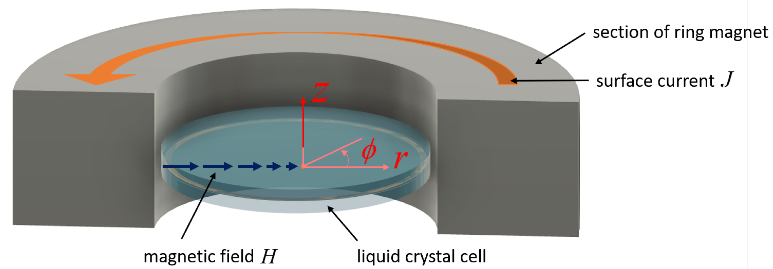
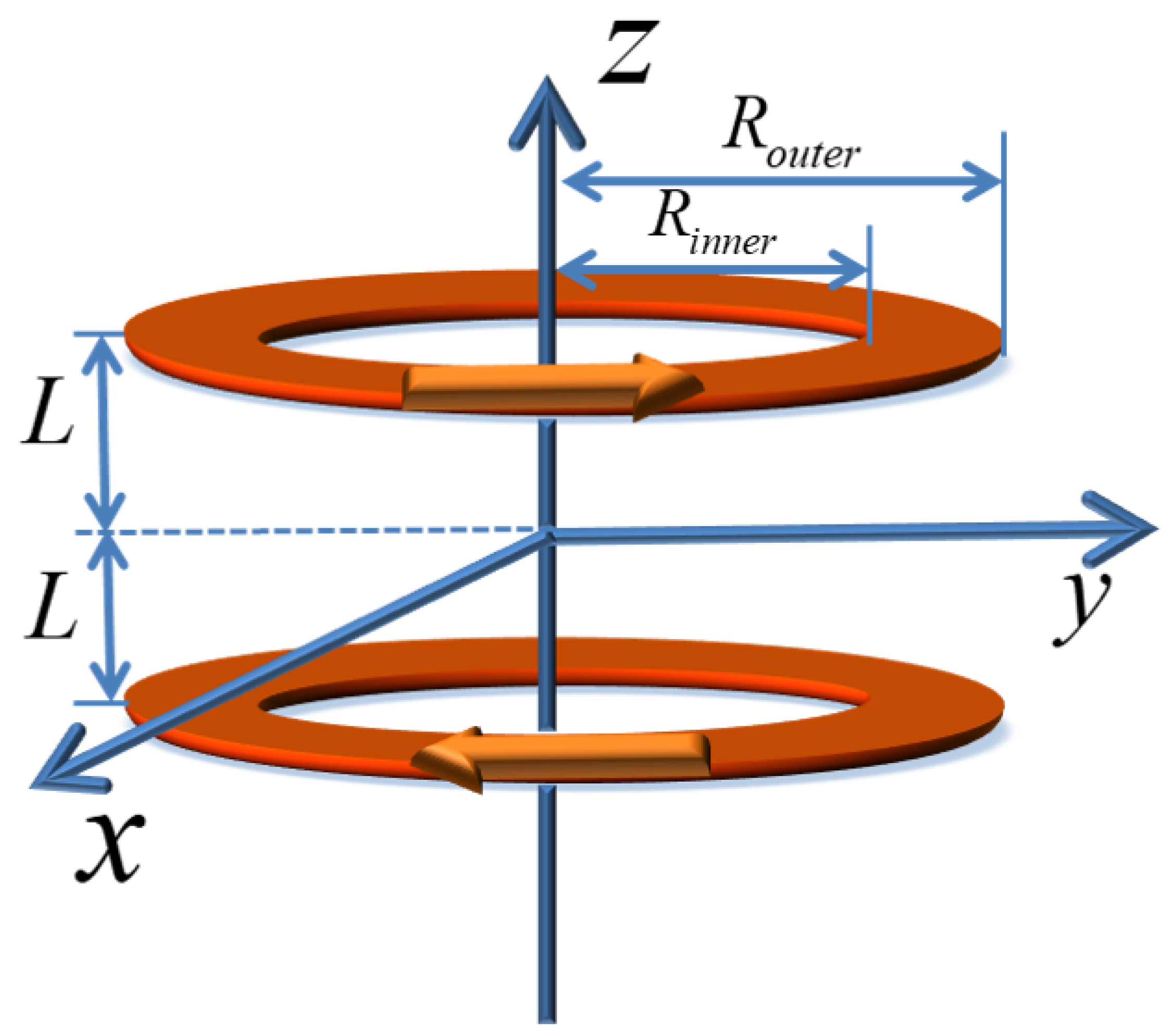
2.1. Ring Magnet

The source of the magnetic field was a ring magnet consisting of twelve wedge-shaped N50 rare-earth neodymium magnets with dimensions (49.95 mm OD × 26.00 mm ID × 11.50 mm thickness) purchased from Supermagnetman.net. The magnet generates a very nearly radially symmetric magnetic field, pointing from the edge towards the center. In the midplane of the ring magnet, the magnitude of the field varies along the radial direction decreasing to zero at the center of the ring. The magnet, with its axis vertical, as shown in Figure 2, was mounted on an xyz stage. It can be translated in the z-direction to apply the magnetic field to the coaxial sample cell.

A LakeShore Model 450 Gaussmeter with a Hall probe was used to measure the field strength of the ring magnet. The probe was mounted on a translation stage; the field was measured as a function of radial position.

2.2. Circular Liquid Crystal Cell

The liquid crystal cell consisting of two circular borosilicate glass substrates (25 mm OD × 0.1 cm) separated by 50 μm annular Mylar film spacers and held together with Norland 65 adhesive was designed to fit into the central cavity of the ring magnet. The cell was filled with 4-cyano-4-pentylbiphenyl (5CB) via capillary action. Strong homeotropic surface alignment was obtained using silane (DMOAP) [9].

2.3. Optical Setup

The nematic director in the magnetic field was studied using optical interferometry. A spatial filter was used to obtain a clean, well aligned beam from a Melles Griot 5 mW laser at 543.5 nm along the symmetry axis of the cell. The beam was expanded and collimated to the diameter of the cell. The cell and the magnet were placed between two crossed polarizers. Interference patterns were recorded as the magnet was translated along the beam. The sample was at room temperature. The position of the magnet relative to the cell was measured and recorded manually while the interference pattern was displayed on a screen and captured using a Canon EOS Rebel T2i camera.

3. Theory

3.1. Modeling Magnetic Field

The radially symmetric magnetic field was generated by a ring formed from truncated wedge-shaped rare-earth magnets. Each magnet is viewed as a surface current loop. Due to cancellation of surface currents at the contact planes, there are two current annuli flowing in opposite directions (counterclockwise and clockwise) on top and bottom of the ring magnet as shown in Figure 3.

The magnetic field is calculated for each current loop using numerical integration of the Biot–Savart law,

$$\mathbf{B}\left(\mathbf{r}\right)=\frac{{\mu }_0}{4\pi }J{\int }_{R_{inner}}^{R_{outer}}{\int }_0^{2\pi }\frac{\widehat{\mathbf{J}}\times \widehat{{\mathbf{r}}^{\prime }}}{{r\prime }^2}Rd\varphi dR,$$

(4)

where $\mathbf{J}$ is the surface current density, ${\mathbf{r}}^{\prime }$ is the vector from the current element to the point $\mathbf{r}$ where $\mathbf{B}$ is specified and $\varphi$ is the azimuthal angle.

3.2. Modeling and Numerics for the Director Field

The director field, in cylindrical coordinates, is

$$\widehat{\mathbf{n}}=\left(sin\theta ,0,cos\theta \right),$$

(5)

where $\theta =\theta \left(r,z\right)$ is the angle between the director and the glass substrate normal.

The free energy is

$$F_{total}={\int }_V\left({\mathcal{F}}_{elastic}+{\mathcal{F}}_{mag}\right)dV,$$

(6)

and in the one constant approximation, the elastic energy density is given by

$${\mathcal{F}}_{elastic}=\frac{1}{2}K\left(\frac{1}{r^2}{sin}^2\theta +{\left(\frac{\partial \theta }{\partial z}\right)}^2+{\left(\frac{\partial \theta }{\partial r}\right)}^2-\frac{2}{r}\frac{\partial \theta }{\partial z}{sin}^2\theta +\frac{2}{r}\frac{\partial \theta }{\partial r}sin\theta cos\theta \right).$$

(7)

When the cell is in the midplane, $\mathbf{H}=-H_r\widehat{\mathbf{r}}$ and

$${\mathcal{F}}_{mag}=-\frac{1}{2}{\mu }_o\Delta \chi H_r^2{sin}^2\theta ,$$

(8)

where ${\mu }_0$ is the permeability of free space, and $\Delta \chi$ is the diamagnetic susceptibility anisotropy. Since the system has cylindrical symmetry and the cell is thin, the variation of H in the z-direction was neglected.

Setting the dissipation rate equal to the rate of change of free energy gives the dynamics for the approach to equilibrium. This gives the equation of motion

$$\gamma \dot{\theta }=\frac{{\partial }^2\theta }{\partial z^2}+\frac{{\partial }^2\theta }{\partial r^2}+\frac{1}{r}\frac{\partial \theta }{\partial r}-\frac{1}{2r^2}sin2\theta +\frac{1}{2}{\alpha }_r^{2}sin2\theta ,$$

(9)

where $\gamma$ is a viscosity and

$${\alpha }_r=\sqrt{\frac{{\mu }_o\Delta \chi }{K}}{H}_r=\frac{\pi }{d}\frac{H_r}{H_c},$$

(10)

where K is the elastic constant. Boundary conditions are $\theta (0,z)=\theta (R,z)=0$ and $\theta (r,d/2)=\theta (r,-d/2)=0$.

Equation (9) was solved numerically using a finite difference and forward time stepping method [9]. A $5\times 200$ square z-r grid was used in the discretization. Initial conditions were biased random orientation of the director on the lattice sites to prevent domain formation in the sample. The numerics was implemented in Visual Fortran, and starting from initial conditions, the code was executed until the mean squared change in $\theta$ was below the threshold in the range of ${10}^{-14}$–${10}^{-16}$.

3.3. Modeling Light Propagation

In the experiment, polarized monochromatic light is normally incident on the sample and propagates along the symmetry axis. The sample is anisotropic and inhomogeneous, so analytic solutions are not available, and the inhomogeneity makes the numerics challenging. Approximations are therefore made in the model to make the problem tractable.

To calculate the transmitted intensity, it is convenient to work with the electric displacement $\mathbf{D}$ instead of the electric field, since for a plane wave with wave vector $\mathbf{k}=(2\pi /\lambda )\widehat{\mathbf{z}}$, $\mathbf{k}·\mathbf{D}=0$. Then, for the incident light polarized along the $\widehat{\mathbf{x}}-$ axis in the lab frame, the incident displacement is given, in terms of the two normal modes, by

$${\mathbf{D}}_{i0}=D_{i0}(\widehat{\mathbf{x}}·\widehat{\mathbf{r}})\widehat{\mathbf{r}}+D_{i0}(\widehat{\mathbf{x}}·\widehat{\mathit{\varphi }})\widehat{\mathit{\varphi }},$$

(11)

where $\varphi$ is the azimuthal angle such that $rcos\varphi =x$, and $\widehat{\mathit{\varphi }}=\widehat{\mathbf{z}}\times \widehat{\mathbf{r}}$. The cell is regarded as being composed of thin parallel nematic layers, with thickness $\Delta$ and layer normal $\widehat{\mathbf{z}}$. The director is in the $z-r$ plane, and $\widehat{\mathbf{n}}·\mathbf{z}=cos\theta$. The refractive index for the mode in the $\widehat{\mathit{\varphi }}$ direction is

$$n_1=n_o,$$

(12)

and for the mode in the $\widehat{\mathbf{r}}$ direction, it is

$$n_2=\frac{n_e{n}_o}{\sqrt{n_e^2{cos}^2\theta +n_o^2{sin}^2\theta }},$$

(13)

where $n_e$ and $n_o$ are the principal refractive indices of the liquid crystal. The sample is assumed to be non-absorbing in the visible, and hence the effect of propagation through a layer is only the acquisition of phase. Reflections have been ignored. The ordinary mode along $\widehat{\mathit{\varphi }}$ acquires phase

$${\delta }_1=\frac{2\pi n_o}{{\lambda }_0}d,$$

(14)

while the extraordinary mode along $\widehat{\mathbf{r}}$ acquires phase

$${\delta }_2=\frac{2\pi n_o}{{\lambda }_0}d\sum _j\frac{n_e}{\sqrt{n_e^2{cos}^2{\theta }_j+n_o^2{sin}^2{\theta }_j}}\frac{\Delta }{d},$$

(15)

where ${\lambda }_0$ is the free space wavelength and j refers to the $j^{th}$ nematic layer.

The light transmitted through the cell passes through the analyzer in the $\widehat{\mathbf{y}}$ direction, and the transmitted displacement is

$${\mathbf{D}}_t=D_{t0}(e^{i{\delta }_2}(\widehat{\mathbf{x}}·\widehat{\mathbf{r}})(\widehat{\mathbf{y}}·\widehat{\mathbf{r}})+e^{i{\delta }_1}(\widehat{\mathbf{x}}·\widehat{\mathit{\varphi }})(\widehat{\mathbf{y}}·\widehat{\mathit{\varphi }})\widehat{\mathbf{y}}.$$

(16)

Since the intensity is proportional to ${\mathbf{DD}}^{*}$, it is given by

$$I=I_0{sin}^2\left(\frac{{\delta }_2-{\delta }_1}{2}\right){sin}^{2}2\varphi .$$

(17)

At a given point $(x,y)$, $\varphi$ satisfies

$$sin2\varphi =\frac{2xy}{x^2+y^2}.$$

(18)

Since $\theta \left(r\right)$ is known from simulations, the refractive indices $n_1$ and $n_2$ and the phase shifts ${\delta }_1$ and ${\delta }_2$ can be determined, and the transmitted intensity at each point can be calculated.

4. Results

4.1. Experiment and Numerics

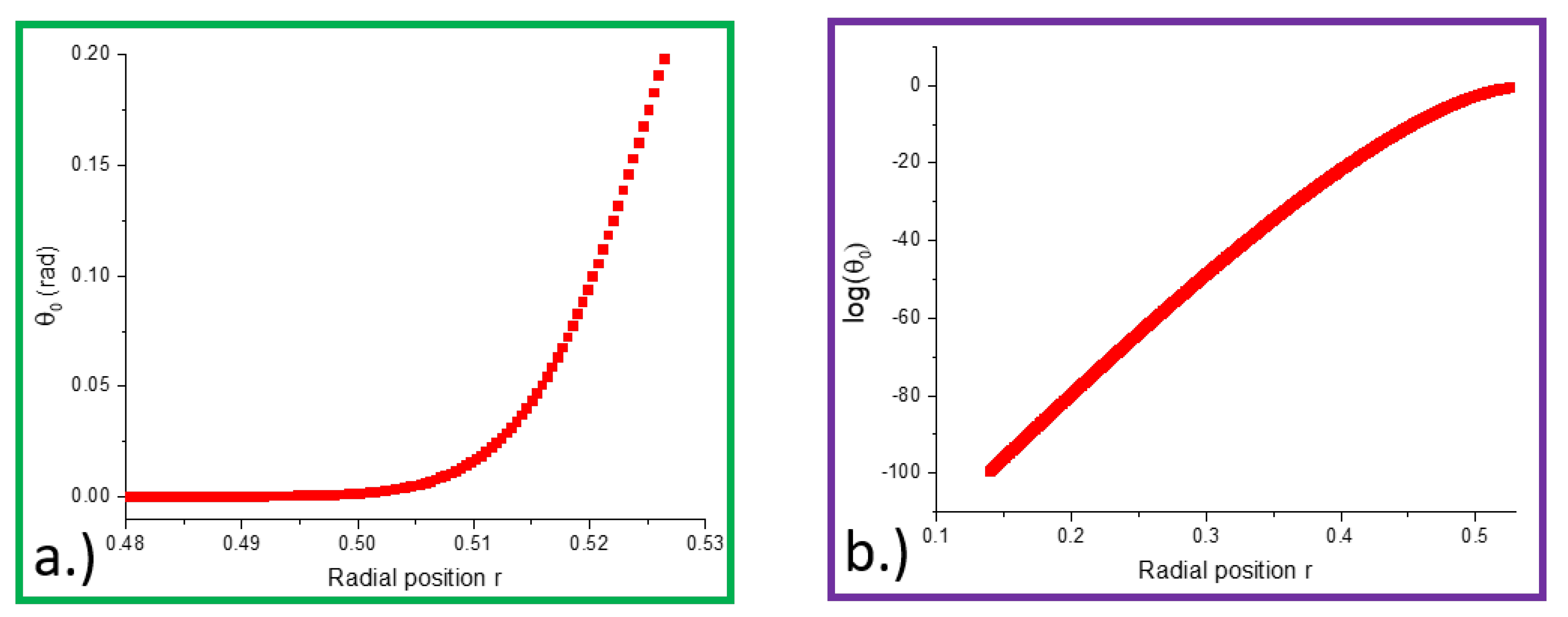
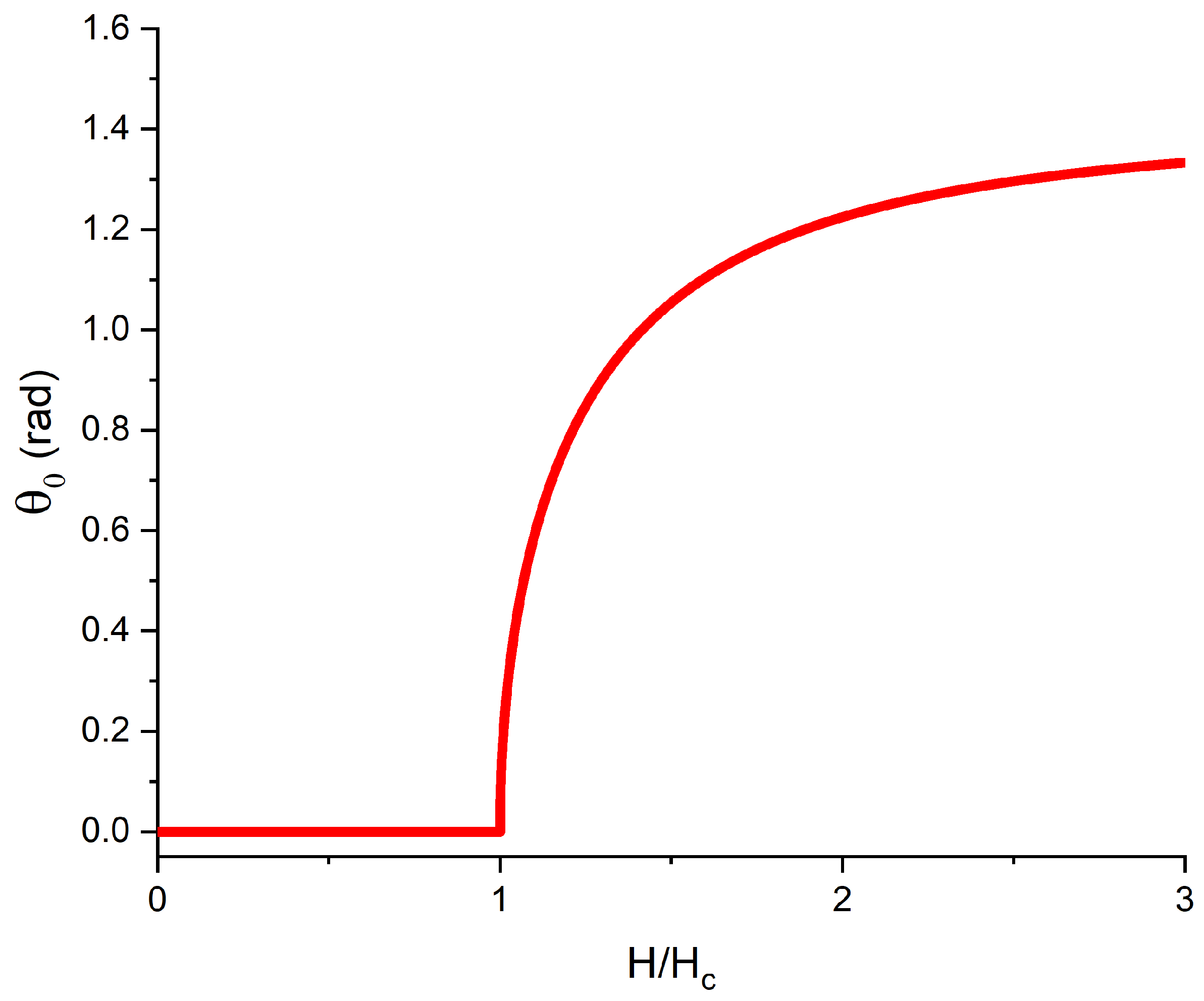
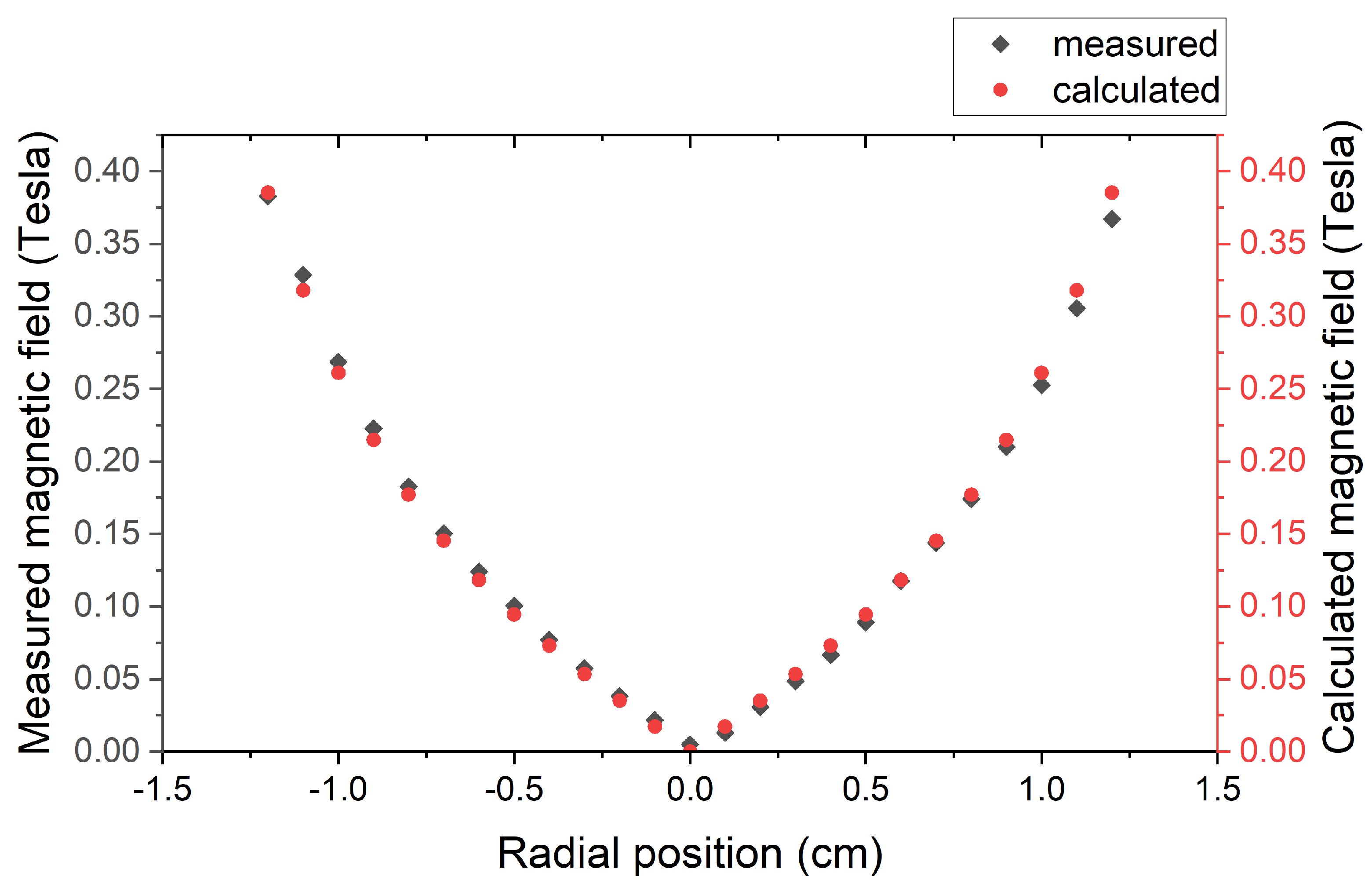
4.1.1. B Field Measurements

The calculated and measured magnetic fields in the midplane as a function of radial position are shown in Figure 4; they agree to with $6\%$. The field is zero at the center due to symmetry and increases initially linearly with radius r.

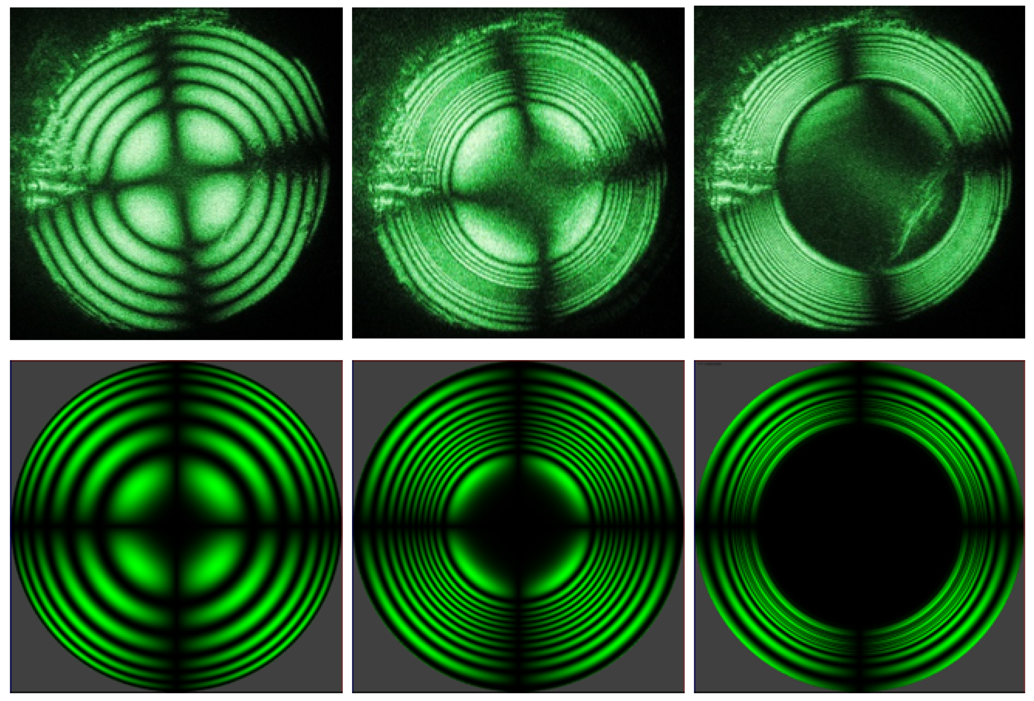
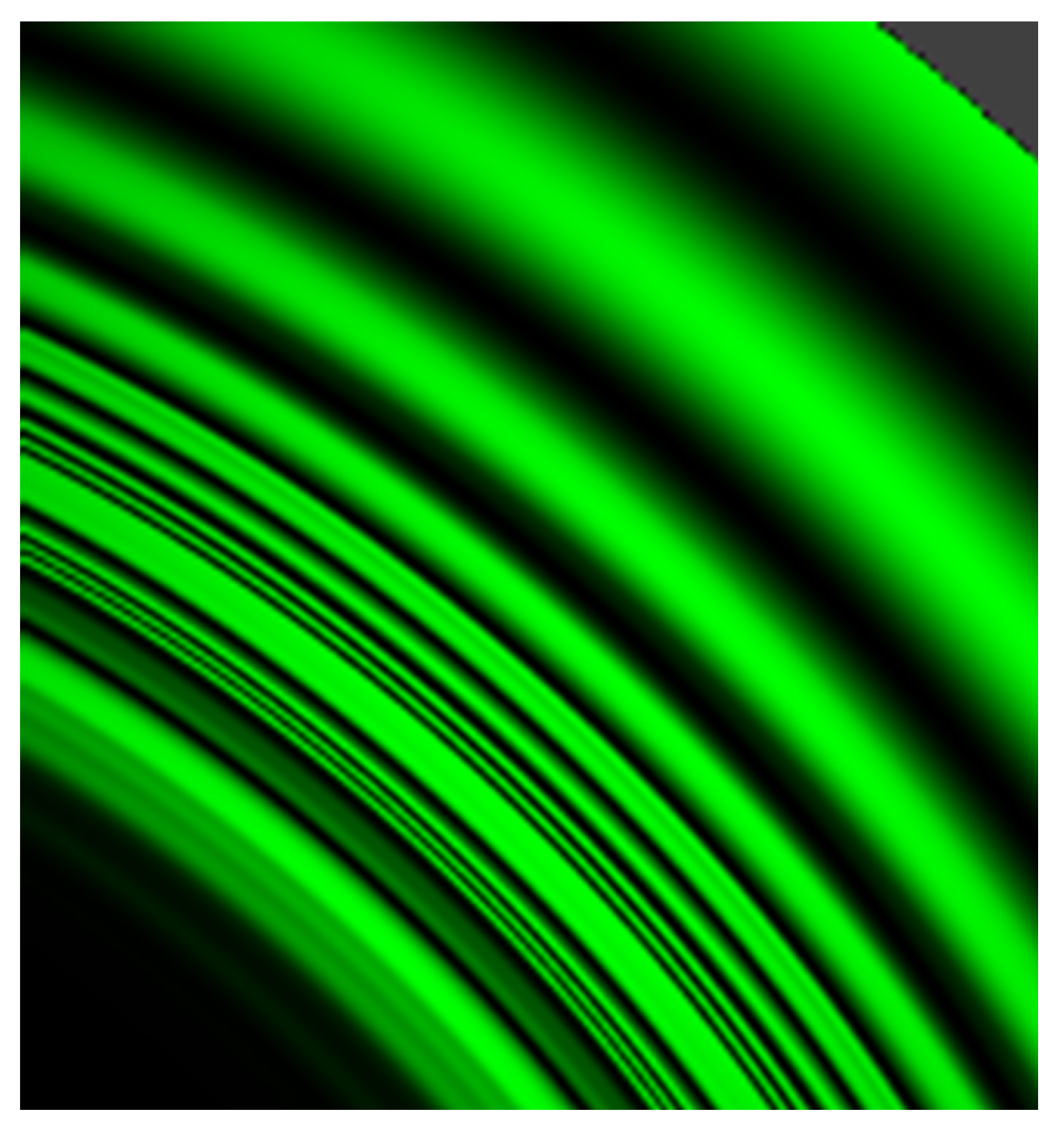
4.1.2. Interference Patterns

Observed and calculated interference patterns for different cell positions, relative to the ring magnet, in the z-direction, are shown in Figure 5.

Magnified far field interference patterns on a screen were observed and photographed (top row) in Figure 5 as the magnet was translated along the symmetry axis. On either side of the midplane, the magnetic field has nonzero z components, as does the director field. The pattern on the left was captured when the sample was outside the ring, the pattern in the middle is when the sample is in the ring, but not yet at the midplane, and the pattern on the right is when the sample is in the midplane. The corresponding patterns on the bottom row in Figure 5 are calculated, based on the director field configuration obtained from energy minimization [9,10].

An enlarged version of the computer-generated interference pattern is shown in Figure 6 to indicate details of the structure.

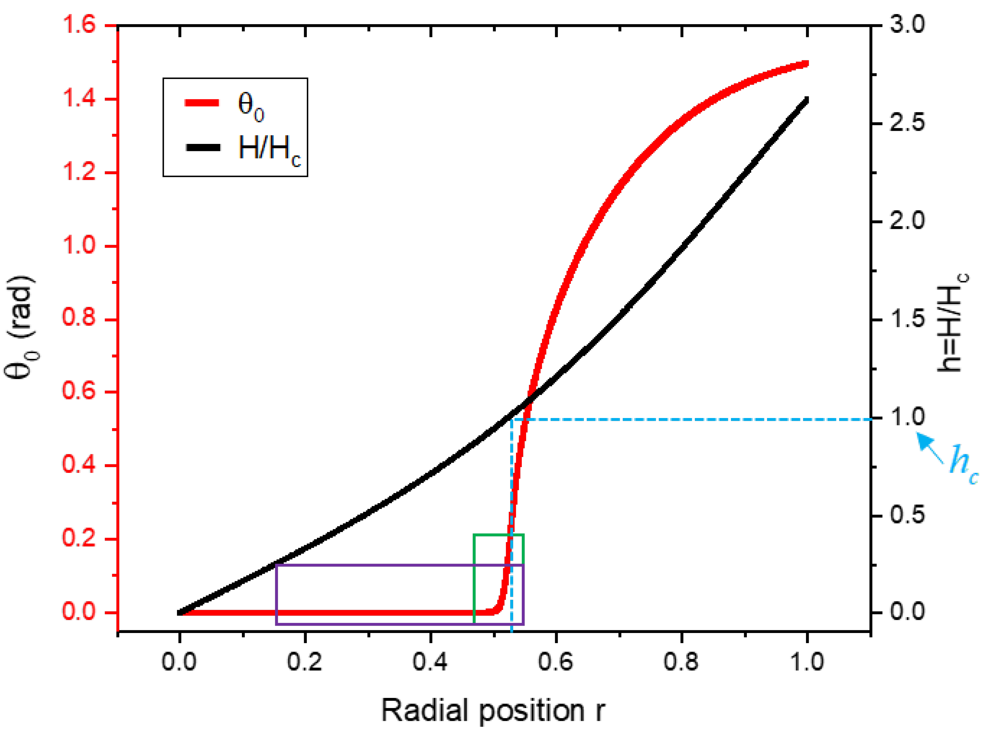
4.1.3. Director Field

Determination of the director pattern in the spatially varying field is the central aspect of this work. With the sample at the midplane of the ring magnet, Figure 7 shows the director angle ${\theta }_0$ in the midplane of the sample, half-way between the plates. The magnetic field is radial, increasing monotonically with r as shown. The angle ${\theta }_0$ changes rapidly in the vicinity of $r=0.5$ where the field $H\approx 0.9H_c$ is below the critical value. Although superficially the plot of ${\theta }_0$ vs. r is similar to Figure 1, as the magnified portions in Figure 8 indicate, instead of falling abruptly to zero, ${\theta }_0$ decreases more slowly, the curvature of the curve changes sign as seen clearly in Figure 8b, and although ${\theta }_0$ is small, it is nonzero, decreasing apparently exponentially as shown in Figure 8a towards the origin.

In Figure 5, the experimental top right figure suggests light transmission—hence nonzero ${\theta }_0$—near the inner boundary of the central dark region, becoming fainter towards the center, in qualitative agreement with Figure 8b.

4.2. Discussion

We begin by noting that the region of interest in our cell is the vicinity of the point where $H=H_c$, which is near r = 5 mm. We believe that in this region, in our thin cell with d = 50 μm , the difference between the cylindrical coordinate and a Cartesian one is negligible, hence we disregard the effects of cylindrical geometry.

Our results indicate that in our cell with strong homeotropic orientation, the director remained partially aligned with the radial magnetic field even in those regions of space where the magnetic field amplitude was below the critical value $H_c$. That is to say, unlike in the case of the classical Freedericksz transition, here $\widehat{\mathbf{H}}·\widehat{\mathbf{n}}\ne 0$ for all $H<H_c$; the spatial variation of the field amplitude has therefore fundamentally changed the nature of the transition. The reason for the change can be understood from elementary considerations. At large values of r, near the outer edge of the cell, the field is strong; $H\gg H_c$ and the director field in the midplane of the cell is expected to be well aligned with the field, as in the classical case in Equation (1). Nearer the center, the field magnitude is reduced, and hence the alignment will also be reduced, as in the classical case. In the region where H is just above $H_c$, however, ${\theta }_0$ cannot depend on the field as in Equation (1); if it did, the gradient of the director field would diverge with diverging elastic energy density. So instead of abruptly decreasing to zero, ${\theta }_0$ must decrease gradually, as shown in Figure 8b. Numerics indicates that the decrease remains gradual and exponential-like, as suggested by Figure 8a.

More formally, since the field H depends on position, ${\theta }_0$ will depend on position, and if $\theta (r,z)={\theta }_0\left(r\right)cos\left(qz\right)$, the dimensionless mean free energy density becomes, for small ${\theta }_0$, after integrating over $z,$

$$\mathcal{F}=\frac{1}{2}{\theta }_0^2(1-\frac{H^2}{H_c^2})+\frac{d^2}{{\pi }^2}{\left(\frac{\partial {\theta }_0}{\partial r}\right)}^2.$$

(19)

To describe the spatial variation of H, we define $x=(r-r_c)/r_c$, so that $x=0$ is the location in the cell where $H=H_c$. In this vicinity, x is small, and then, to a good approximation,

$$H^2=H_c^2(1+x).$$

(20)

The Euler-Lagrange equation minimizing the free energy in Equation (19) then becomes

$$\frac{\partial {\theta }_0^2}{\partial x^2}=-{\left(\pi \frac{r_c}{d}\right)}^2{\theta }_{0}x.$$

(21)

The solutions are Airy functions, shown in Figure 9.

Since $ai$ dominates,

$${\theta }_0\left(x\right)\simeq ai(-\gamma x),$$

(22)

where

$$\gamma ={\left(\pi \frac{r_c}{d}\right)}^{\frac{2}{3}}.$$

(23)

Since $r_c=0.52$ corresponds to $6.6$ mm, $\gamma =56$. We note that $ai(\gamma (r_c-r)/r_c)$ is in good agreement with the gradual decrease of ${\theta }_0\left(r\right)$ with decreasing r near $r_c$ as seen in Figure 8b, and the asymptotics for large $-x$ is exponential-like decay as seen in Figure 8a. Although it appears that ${\theta }_0$ decays to zero at the origin (but not before), this has not been confirmed. As Figure 8a indicates, the values of ${\theta }_0$ near the origin are extremely small, and in the numerical computation of the director field, the relaxation of Equation (9) is extremely slow. We are not yet therefore certain, but the indications are that ${\theta }_0$ indeed decays to zero at the origin. The spatial variation of the magnetic field therefore ‘lifts’ the system from the transition, and if the magnetic field is not homogeneous, there are no discontinuities either in the director field, or in its derivatives. This is reminiscent of the effect of an electric or magnetic field on the temperature driven nematic-isotropic phase transition; the presence of the field makes the order parameter everywhere nonzero, and it and its derivatives continuous.

5. Conclusions

The response of a nematic cell in a spatially varying magnetic field was explored experimentally and theoretically. The magnetic field with cylindrical symmetry was generated by a series of wedge-shaped rare-earth magnets forming a ring. The strength of the field in the radial direction in the midplane of the ring magnet was measured and calculated. The director configuration of a homeotropically aligned nematic in this field was probed using interferometry. The director field was modeled using the Oseen-Frank theory, and determined numerically via an energy minimizing scheme. Agreement of the calculated and measured interference patterns verified the calculated director field. Of particular interest in this project was the behavior of the nematic director in the region where the magnetic field magnitude is near the critical field value in the classical Freedericksz transition. The results indicate a smoothly varying director field everywhere, with no evidence of discontinuities of the director angle or its derivatives. Although the director field studied here differs only slightly from what it would be in a uniform field with the same magnitude, the director field changes smoothly with position everywhere in the regions studied. The effect of the spatial variation of the magnetic field is the absence of discontinuities; in a spatially varying field therefore there is no Freedericksz transition. We anticipate equivalent result in planar aligned rather than homeotropic cells, in the case of electric rather than magnetic field induced transitions, in the case of wedge cells and in other analogous system.

References

- Mauguin, C. On O. Lehmann’s liquid crystal. Phys. Z 1911, 12, 1011–1015. [Google Scholar]
- Mauguin, C. Orientation of liquid crystals by strips of mica. Compte-Rendus Hebdomadaires Séances l’Académie Sciences 1913, 156, 1246–1247. [Google Scholar]
- Freedericksz, V.; Zolina, V. Forces causing the orientation of an anisotropic liquid. Trans. Faraday Soc. 1933, 29, 919–930. [Google Scholar] [CrossRef]
- Frank, F.C. On the Theory of Liquid Crystals. Discuss. Faraday Soc. 1958, 25, 19–28. [Google Scholar] [CrossRef]
- Kini, U.D. Generalized Fréedericksz transition in nematics. Geometrical threshold and quantization in cylindrical geometry. J. Phys. 1988, 49, 527–539. [Google Scholar] [CrossRef]
- Oswald, P.; Pieranski, P. Nematic and Cholesteric Liquid Crystals: Concepts and Physical Properties Illustrated by Experiments; Taylor & Francis: Boca Raton, FL, USA, 2005; pp. 131–138. [Google Scholar]
- Gennes, P.G.d.; Prost, J. The Physics of Liquid Crystals, 2nd ed.; Clarendon Press: Oxford, UK; Oxford University Press: New York, NY, USA, 1995; pp. 123–133. [Google Scholar]
- Landau, L.D. On the Theory of Phase Transitions. Zh. Eksp. Teor. Fiz. 1937, 7, 19–32. [Google Scholar] [CrossRef]
- Guo, T. Using Light to Study Liquid Crystals and Using Liquid Crystals to Control Light. Ph.D. Thesis, Kent State University, Kent, OH, USA, 2020. [Google Scholar]
- Guo, T.; Palffy-Muhoray, P. Interferometric studies of nematic liquid crystals in an inhomogeneous magnetic field. Mol. Cryst. Liq. Cryst. 2017, 647, 196–200. [Google Scholar] [CrossRef]
Publisher’s Note: MDPI stays neutral with regard to jurisdictional claims in published maps and institutional affiliations. |
© 2021 by the authors. Licensee MDPI, Basel, Switzerland. This article is an open access article distributed under the terms and conditions of the Creative Commons Attribution (CC BY) license (https://creativecommons.org/licenses/by/4.0/).
Share and Cite
Guo, T.; Zheng, X.; Palffy-Muhoray, P. The Freedericksz Transition in a Spatially Varying Magnetic Field. Crystals 2021, 11, 541. https://doi.org/10.3390/cryst11050541
Guo T, Zheng X, Palffy-Muhoray P. The Freedericksz Transition in a Spatially Varying Magnetic Field. Crystals. 2021; 11(5):541. https://doi.org/10.3390/cryst11050541
Chicago/Turabian StyleGuo, Tianyi, Xiaoyu Zheng, and Peter Palffy-Muhoray. 2021. "The Freedericksz Transition in a Spatially Varying Magnetic Field" Crystals 11, no. 5: 541. https://doi.org/10.3390/cryst11050541
APA StyleGuo, T., Zheng, X., & Palffy-Muhoray, P. (2021). The Freedericksz Transition in a Spatially Varying Magnetic Field. Crystals, 11(5), 541. https://doi.org/10.3390/cryst11050541