Multi-Task Regression Model for Predicting Photocatalytic Performance of Inorganic Materials

Abstract

As renewable energy technologies advance, identifying efficient photocatalytic materials for water splitting to produce hydrogen has become an important research focus in materials science. This study presents a multi-task regression model (MTRM) designed to predict the conduction band minimum (CBM), valence band maximum (VBM), and solar-to-hydrogen efficiency (STH) of inorganic materials. Utilizing crystallographic and band gap data from over 15,000 materials in the SNUMAT database, machine-learning methods are applied to predict CBM and VBM, which are subsequently used as additional features to estimate STH. A deep neural network framework with a multi-branch, multi-task regression structure is employed to address the issue of error propagation in traditional cascading models by enabling feature sharing and joint optimization of the tasks. The calculated results show that, while traditional tree-based models perform well in single-task predictions, MTRM achieves superior performance in the multi-task setting, particularly for STH prediction, with an MSE of 0.0001 and an R² of 0.8265, significantly outperforming cascading approaches. This research provides a new approach to predicting photocatalytic material performance and demonstrates the potential of multi-task learning in materials science.

1. Introduction

Since Fujishima and Honda first reported in 1972 that TiO₂ electrodes could split water under ultraviolet light [1], photocatalysis has attracted extensive attention as a clean technology capable of directly converting solar energy into chemical energy. In particular, photocatalytic hydrogen production—using sunlight to split water into hydrogen and oxygen—represents a promising strategy for sustainable energy development [2]. However, the solar-to-hydrogen (STH) conversion efficiency of traditional photocatalysts remains far below the threshold required for practical applications. Moreover, the discovery and optimization of these materials largely depend on inefficient and time-consuming trial-and-error approaches, which demand significant human and material resources [3,4]. In recent years, the rapid progress of machine learning (ML) in materials science and chemistry has opened new possibilities for improving photocatalytic hydrogen production. As a core branch of artificial intelligence, ML excels at identifying patterns in large datasets and making complex predictions [5]. In photocatalysis, ML enables rapid screening of potential materials from vast libraries, prediction of their optoelectronic properties, and optimization of reaction conditions—significantly accelerating the discovery of high-performance photocatalysts [6,7].

For example, Zhou et al. developed an ML framework to systematically screen metal oxide photocatalysts for hydrogen production. By integrating material databases, ML prediction, and density functional theory (DFT) validation, they identified ten promising candidates, including CsYO₂ [8]. Wang et al. introduced a funnel-like screening strategy that combines ML with first-principles modeling to discover efficient two-dimensional photocatalysts, focusing on optimizing their chemical and electronic properties [9]. The integration of ML with photocatalysis has led to efficient research strategies. In material screening, high-throughput computing allows for the rapid evaluation of thousands of candidate compounds. Tao et al., for instance, used a neural network to screen over 30,000 perovskite structures, identifying materials that could boost hydrogen yield by 6.4% [10]. For performance prediction and optimization, deep learning models help accurately forecast catalytic efficiency and guide reaction condition tuning. Zheng et al. developed a gated recurrent unit (GRU) neural network that outperformed traditional kinetic models in predicting hydrogen production rates [11]. Additionally, combining ML with traditional computational methods, such as quantum machine learning (QML), has further improved catalyst design efficiency [12].

In photocatalytic hydrogen production, band edge positions are critical indicators of material performance. Specifically, the conduction band minimum (CBM) and valence band maximum (VBM) determine whether photocatalytic reactions can proceed [13]. To efficiently predict these values for non-metallic materials, Kiyohara et al. proposed an ML model using bulk and surface structural data to forecast band edge positions of oxide surfaces, enabling large-scale materials analysis and design [14]. For effective water splitting, the CBM must lie below the hydrogen reduction potential (0 V vs. NHE, pH = 0), while the VBM must exceed the oxygen evolution potential (1.23 V vs. NHE, pH = 0) [15]. Beyond band positions, the STH conversion efficiency is another core metric, influenced by optical absorption, charge carrier utilization, and overpotentials. Together, these factors allow for a rapid evaluation of a material’s photocatalytic potential [16,17]. If CBM, VBM, and STH could be reliably predicted from material structure and composition using ML, it would greatly enhance the efficiency of screening and evaluating photocatalysts. Although several databases have compiled information on structure, composition, and band gaps [18,19,20], data on vacuum-referenced CBM, VBM, and STH remain limited. Prior studies have used features such as elemental composition, electronegativity, and band gap to predict CBM and VBM relative to the vacuum level [21]. Meanwhile, considering light absorption and charge carrier utilization provides a physical foundation for STH prediction [16]. In this study, we construct a dataset using band gaps, structural, and compositional information from the SNUMAT materials database, along with vacuum-level-referenced CBM and VBM, and a theoretical model for STH. We then develop an end-to-end, multi-task joint neural network to simultaneously predict CBM, VBM, and STH. This model employs shared fusion layers to jointly optimize the three tasks, aiming to reduce error propagation and enhance generalization performance. The novelty of this work lies in the unified multi-task learning framework that simultaneously predicts CBM, VBM, and STH from material features, offering a more comprehensive and physically grounded strategy for high-throughput photocatalyst screening.

2. Data Acquisition and Feature Construction

The initial dataset used in this study is primarily derived from the SNUMAT database, developed by the Ulsan National Institute of Science and Technology (UNIST). SNUMAT is a comprehensive materials science platform that provides crystallographic and electronic property data for over 15,000 inorganic compounds [20]. It serves as a valuable resource for computational materials research and industrial applications, particularly in the fields of energy materials and semiconductors.

From this database, we extracted both the crystal structures and band gap information for more than 15,000 inorganic materials in the Support Material (SI data). The band gap values were computed using the high-accuracy HSE06 hybrid functional, known for its close agreement with experimental results, making it highly suitable for reliable property prediction [22].

Building upon the obtained band gap data, we calculated the valence band maximum (VBM) and conduction band minimum (CBM) positions for each compound. These values were estimated using the material’s chemical composition, the Mulliken electronegativities of the constituent elements, and established empirical formulas.

For a material to be viable for photocatalytic water splitting, its electronic band structure must meet specific thermodynamic criteria: the CBM must lie above (i.e., more negative than) the reduction potential of water (H⁺/H₂), while the VBM must lie below (i.e., more positive than) the oxidation potential (H₂O/O₂). The band edge positions can be estimated using the following empirical relations [21]:

$$E_{CBM}=\chi -E_0-{\displaystyle \frac{E_g}{2}}$$

$$E_{VBM}=\chi -E_0+{\displaystyle \frac{E_g}{2}}$$

Here, E_g is the band gap, E₀ = 4.5, eV is the reference vacuum level, and χ is the material’s average electronegativity, calculated as

$$\chi ={\left(\prod _{i=1}^n{\chi }_i^{N_i}\right)}^{1/N}$$

where χ_i is the electronegativity of the i-th element, N_i is its atomic count in the compound, N is the total number of atoms, and n is the number of element types.

After determining the conduction band minimum (CBM) and valence band maximum (VBM) positions, we evaluated each material’s potential for photocatalytic hydrogen production. Specifically, if the material’s band edges do not straddle the redox potentials of water (i.e., CBM < H⁺/H₂ or VBM > H₂O/O₂), the material is considered unsuitable, and its solar-to-hydrogen efficiency (STH) is set to zero. If the CBM and VBM positions satisfy the necessary energetic alignment—i.e., the band gap covers the water redox window—the material is deemed potentially active. In such cases, the STH value is estimated using a physical model proposed in [16].

$${\eta }_{STH}={\eta }_{abs}\cdot {\eta }_{cu}$$

This model incorporates the effects of solar absorption, charge carrier generation, and transport efficiency. The terms ${\eta }_{abs}$ and ${\eta }_{cu}$ represent the light absorption efficiency and carrier utilization efficiency, respectively.

$${\eta }_{abs}={\displaystyle \frac{{\int }_{E_g}^{\mathrm{\infty }}P\left(\mathrm{\hslash }\omega \right)d\left(\mathrm{\hslash }\omega \right)}{{\int }_0^{\mathrm{\infty }}P\left(\mathrm{\hslash }\omega \right)d\left(\mathrm{\hslash }\omega \right)}}$$

$${\eta }_{cu}={\displaystyle \frac{\mathsf{\Delta }G\cdot {\int }_E^{\mathrm{\infty }}\frac{P\left(\mathrm{\hslash }\omega \right)}{\mathrm{\hslash }\omega }d\left(\mathrm{\hslash }\omega \right)}{{\int }_{E_g}^{\mathrm{\infty }}P\left(\mathrm{\hslash }\omega \right)d\left(\mathrm{\hslash }\omega \right)}}$$

$P\left(\mathrm{\hslash }\omega \right)$ represents the photon energy, where ℏω corresponds to the AM1.5G solar spectrum intensity. The denominator indicates the total incident light power density, while the numerator represents the power density of light that the material can absorb. ΔG denotes the free energy of the water splitting reaction (1.23 eV), and E represents the minimum photon energy required to drive the photocatalytic reaction, considering the overpotential.

$$E=\left\{\begin{array}{ll}{E}_g,\left(\chi \left(H_2\right)\ge 0.2,\chi \left(O_2\right)\ge 0.6\right)& \\ E_g+0.2-\chi \left(H_2\right),\left(\chi \left(H_2\right)<0.2,\chi \left(O_2\right)\ge 0.6\right)& \\ E_g+0.6-\chi \left(O_2\right),\left(\chi \left(H_2\right)\ge 0.2,\chi \left(O_2\right)<0.6\right)& \\ E_g+0.8-\chi \left(H_2\right)-\chi \left(O_2\right),\left(\chi \left(H_2\right)<0.2,\chi \left(O_2\right)<0.6\right)& \end{array}\right.$$

In the STH estimation model, χ(H₂) represents the potential difference between the conduction band minimum (CBM) and the H⁺/H₂ reduction potential, while χ(O₂) denotes the potential difference between the valence band maximum (VBM) and the H₂O/O₂ oxidation potential. These two parameters reflect the alignment between a material’s band edges and the water redox window, indicating whether the photo-generated electrons and holes possess sufficient energy to drive hydrogen and oxygen evolution reactions, respectively. The model thus incorporates both solar absorption capability and charge carrier utilization efficiency, providing a physically sound foundation for evaluating photocatalytic hydrogen production potential. Approximately 90.33% of the samples in the dataset exhibit an STH value of zero, while only 9.67% have non-zero values. This pronounced imbalance highlights the fact that only a small fraction of materials meet the stringent band edge alignment criteria required for photocatalytic hydrogen production. With CBM, VBM, and STH values obtained as target variables, we further leveraged materials’ crystal structure and composition information for data-driven analysis. For this purpose, we used Matminer (v0.9.3), a Python library tailored for materials informatics. Matminer supports automated feature extraction from crystal structures and compositions for machine-learning applications [23]. In our case, 256 structure- and composition-based features were generated, forming a comprehensive feature set for model training.

Given that computing CBM and VBM via HSE06-based density functional theory (DFT) is computationally expensive, and yet these variables are critical to photocatalytic performance, we proposed an efficient alternative: first, predict CBM and VBM using machine-learning models, then use these predicted values as additional features to estimate STH. This leads to a multi-task regression framework involving three sub-tasks—predicting CBM, VBM, and STH—which balances computational efficiency with physical interpretability.

3. Model Design

Traditional single-task prediction methods typically perform feature selection based on feature importance, predict CBM and VBM values, and then add CBM and VBM as additional features for predicting STH. In this cascading prediction approach, separate models are usually used to predict CBM and VBM individually, and their prediction results are then fed into the STH model. However, this method suffers from a significant issue of error accumulation. Although the CBM and VBM models, trained independently, perform well individually, their predictions still contain errors. When these predicted values are passed into the STH model, the errors may be further amplified, leading to instability in the final STH prediction performance.

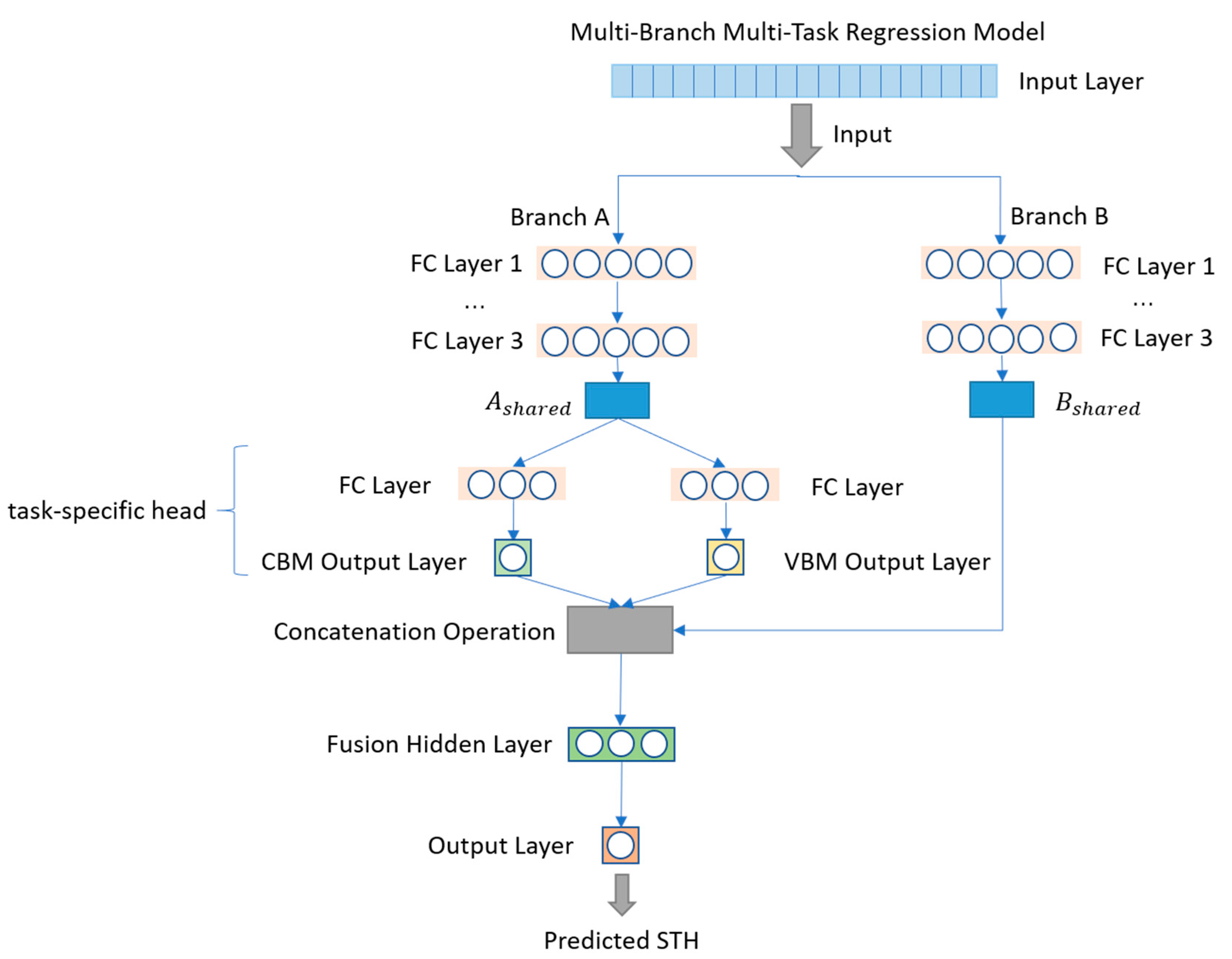
To effectively capture the feature dependencies between different prediction tasks and mitigate the negative impact of error accumulation in traditional cascading methods, this study designs and implements an end-to-end, multi-input, multi-branch joint regression prediction model (multi-task regression model, MTRM). This model is built on a deep neural network framework, with a multi-branch structure to handle the feature information required by each task separately. A fusion layer is used to achieve collaboration and sharing of feature information, thereby jointly optimizing the three tasks (CBM, VBM, and STH). The specific model design is shown in Figure 1. The model consists of the following three main components. The program implementing the proposed model is named MTRM.py and has been included in the Supporting Material.

3.1. Branch A (CBM/VBM Branch)

The input features of Branch A are derived from all the features in the dataset, excluding the target variables (i.e., CBM, VBM, and STH). To effectively extract common features that contribute to CBM and VBM prediction, Branch A uses a three-layer fully connected neural network structure with ReLU activation functions at each layer. These functions non-linearly map the raw inputs to a high-dimensional feature space, enhancing the model’s ability to capture complex nonlinear relationships. The shared feature table is then used to predict the conduction band minimum (CBM) and valence band maximum (VBM) through two independent sub-networks:

$$A_{shared}=ReLU\left(W_3^A\left(ReLU\left(W_2^A\left(ReLU\left(W_1^A{x}_A+b_1^A\right)+b_2^A\right)\right)+b_3^A\right)\right)$$

$$\mathrm{C}\mathrm{B}{\mathrm{M}}_{\mathrm{p}\mathrm{r}\mathrm{e}\mathrm{d}}={\mathrm{W}}_{\mathrm{c}\mathrm{b}\mathrm{m}}\left(\mathrm{R}\mathrm{e}\mathrm{L}\mathrm{U}\left({\mathrm{W}}_{\mathrm{c}\mathrm{b}\mathrm{m}1}{\mathrm{A}}_{\mathrm{s}\mathrm{h}\mathrm{a}\mathrm{r}\mathrm{e}\mathrm{d}}+{\mathrm{b}}_{\mathrm{c}\mathrm{b}\mathrm{m}1}\right)\right)+{\mathrm{b}}_{\mathrm{c}\mathrm{b}\mathrm{m}}$$

$$VB{M}_{pred}=W_{vbm}\left(ReLU\left(W_{vbm1}{A}_{shared}+b_{vbm1}\right)\right)+b_{vbm}$$

where W and b represent the weights and biases of the corresponding layers, and A_shared and B_shared are the shared feature vectors.

Branch A includes three fully connected layers with 256 neurons each (i.e., branch_A_fc1, branch_A_fc2, and branch_A_fc3), followed by two prediction heads: CBM head and VBM head. Each prediction head contains a hidden layer with 128 neurons and a final output layer with a single neuron for scalar prediction.

3.2. Branch B (STH Branch)

The input features of Branch B are identical to those of Branch A. However, Branch B focuses on extracting feature representations that are closely related to the STH prediction task. It also uses a three-layer fully connected structure and ReLU activation functions to perform nonlinear feature mapping:

$$B_{shared}=ReLU\left(W_3^B\left(ReLU\left(W_2^B\left(ReLU\left(W_1^B{x}_B+b_1^B\right)+b_2^B\right)\right)+b_3^B\right)\right)$$

This design allows the model to independently learn feature representations optimized for STH while ensuring compatibility with the fusion of CBM and VBM predictions.

Similar to Branch A, Branch B also includes three fully connected layers with 256 neurons each (i.e., branch_B_fc1 to branch_B_fc3). These layers extract task-specific features that are critical to the STH prediction.

3.3. Fusion Layer

The Fusion Layer is the key innovation of this study. It concatenates the feature representations output from Branch B with the predicted CBM and VBM values from Branch A to generate a fused feature representation. This structural design not only allows the STH prediction to directly utilize the predicted information of CBM and VBM, but also ensures that, during backpropagation, the errors in the STH prediction effectively guide the prediction processes of CBM and VBM, thus achieving collaborative optimization among tasks:

$$Fusio{n}_{input}=\left[B_{shared},CB{M}_{pred},VB{M}_{pred}\right]$$

The fused feature vector is passed through additional fully connected layers and nonlinear mappings to finally output the predicted value for the target variable, STH:

$$ST{H}_{pred}=W_{fusion2}\left(ReLU\left(W_{fusion1}Fusio{n}_{input}+b_{fusion1}\right)\right)+b_{fusion2}$$

With this design, the model achieves true end-to-end optimization during training, with the errors of the STH task being backpropagated through the fusion layer. This drives Branch A to adjust its prediction strategy so that CBM and VBM predictions not only focus on their own accuracy but also actively provide more precise feature inputs for the STH task. This joint optimization mechanism effectively reduces the error propagation and amplification problems seen in traditional cascading methods, significantly improving the model’s overall prediction stability and generalization capability.

The Fusion Layer consists of two fully connected layers: fusion_fc1 with 128 neurons and fusion_fc2 with 1 neuron for the final scalar output.

The study uses the Adam optimizer for end-to-end training with a learning rate of 0.0002 and assigns a higher weight to the STH task loss to enhance the dominance of the STH prediction task in the joint training process, further improving the overall prediction performance. Additionally, fixed random seeds and standardized data preprocessing strategies are set to ensure the reproducibility of the training process and the stability and consistency of the experimental results.

4. Training, Evaluation, and Results Discussion

This study uses Mean Squared Error (MSE) as the loss function for each task. The total loss is computed as the sum of the individual losses for CBM, VBM, and STH, and optimized using the Adam optimizer through backpropagation. Since the model is trained in an end-to-end manner, the error from the STH prediction directly influences the shared layers as well as the CBM/VBM branches, enabling collaborative optimization across all tasks.

After training, we evaluate each task using MSE, RMSE, MAE, and R² scores on the test set. Additionally, to more comprehensively assess the model’s performance in predicting STH, we conduct a further experiment using the entire dataset (including both training and test sets) to make predictions. During inference, only the input features are required, and CBM/VBM are predicted internally. During training, however, the ground-truth CBM/VBM values are used solely for computing the corresponding loss terms and are not fed into the STH branch directly. No ground-truth target values are involved. This evaluation reflects the model’s ability to generalize and maintain stable performance in a fully end-to-end inference pipeline, rather than merely its generalization on a held-out test set. The results showcase the model’s robustness and error control capabilities throughout the joint prediction process.

4.1. Comparison of CBM Prediction Performance

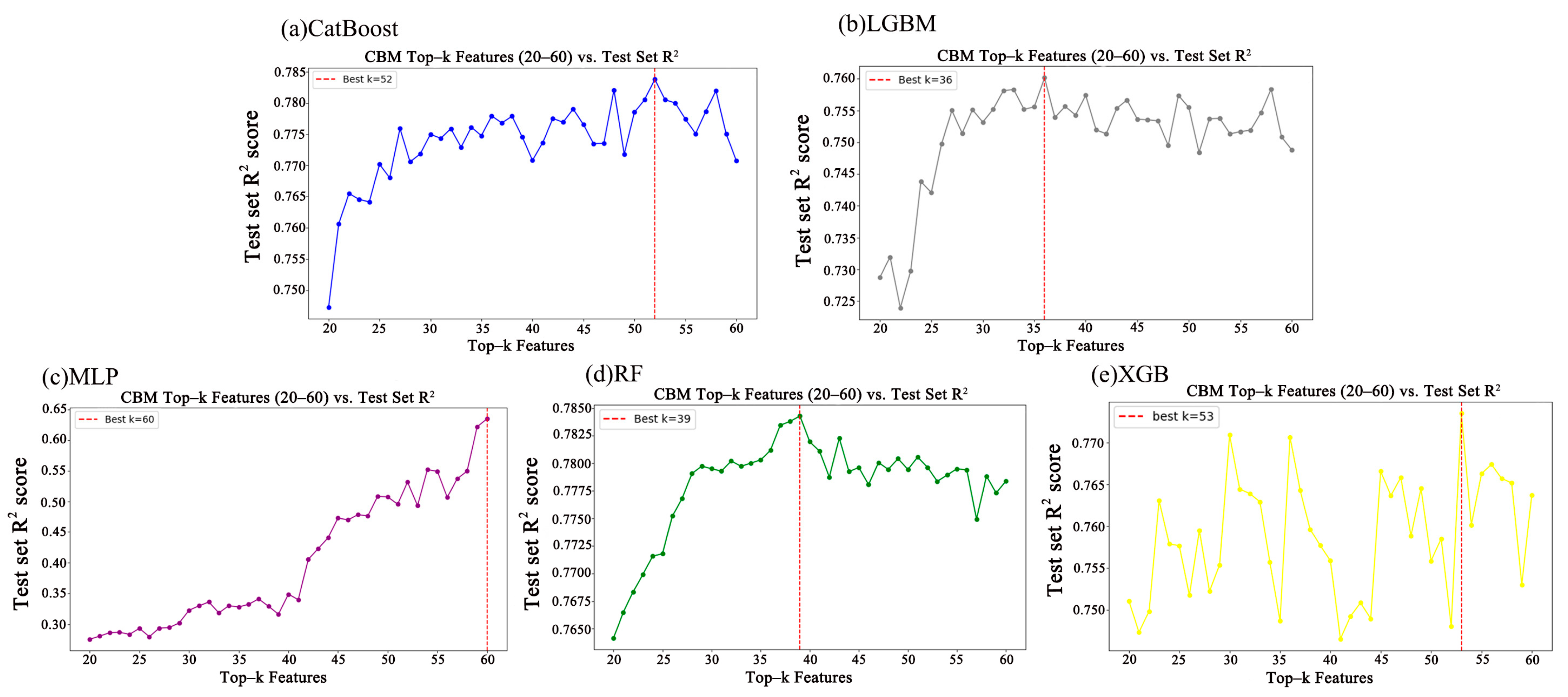
Figure 2 presents the variations in R² scores of five different machine-learning models on the test set, as a function of selected feature counts ranging from 20 to 60. The purpose is to identify an optimal subset of features capable of achieving higher R² scores, which allows us to identify the best possible performance of each model within a reasonable feature range and ensures a fair comparison with our proposed multi-task neural network. The upper limit of 60 was chosen based on the feature importance rankings: beyond this point, the importance scores of the remaining features become negligibly small (less than 0.0000001) across all traditional models, making their contribution to prediction minimal. The lower limit of 20 was selected to ensure sufficient feature diversity while avoiding underfitting.

The CatBoost model (Figure 2a) exhibits fluctuating R² scores with increasing feature numbers, reaching its optimal performance at k = 52k, marked by a red dashed line. The LightGBM model (Figure 2b) displays a steadily increasing trend of R² scores with rising feature counts, achieving its best performance at k = 39. The MLP model (Figure 2c) shows a clear linear increase in R² scores as feature count increases, achieving the highest performance at the maximum considered feature count (k = 60). In the Random Forest (RF) model (Figure 2d), R² scores initially rise with increasing features but decline after peaking at k = 39k, likely due to feature redundancy or overfitting. The XGBoost model (Figure 2e) demonstrates considerable fluctuation in R² scores as feature count increases, with optimal performance at k = 53k, also indicated by a red dashed line.

Table 1. Comparison of Model Performance for CBM Prediction: MSE, RMSE, MAE, and R² Metrics.

Model	MSE	RMSE	MAE	R2
MTRM	0.1928	0.4391	0.2341	0.7497
XGBoost	0.1729	0.4159	0.2159	0.7713
Random Forest	0.1632	0.4039	0.2140	0.7843
MLP	0.2762	0.5256	0.3670	0.6348
CatBoost	0.1635	0.4044	0.2409	0.7838
LightGBM	0.1814	0.4259	0.2604	0.7602

summarizes the regression evaluation metrics (MSE, RMSE, MAE, and R²) for these five traditional machine-learning models. Among them, the Random Forest (R² = 0.7843, MSE = 0.1632) and CatBoost (R² = 0.7838, MSE = 0.1635) models perform the best in CBM prediction, exhibiting strong capability in capturing nonlinear relationships.

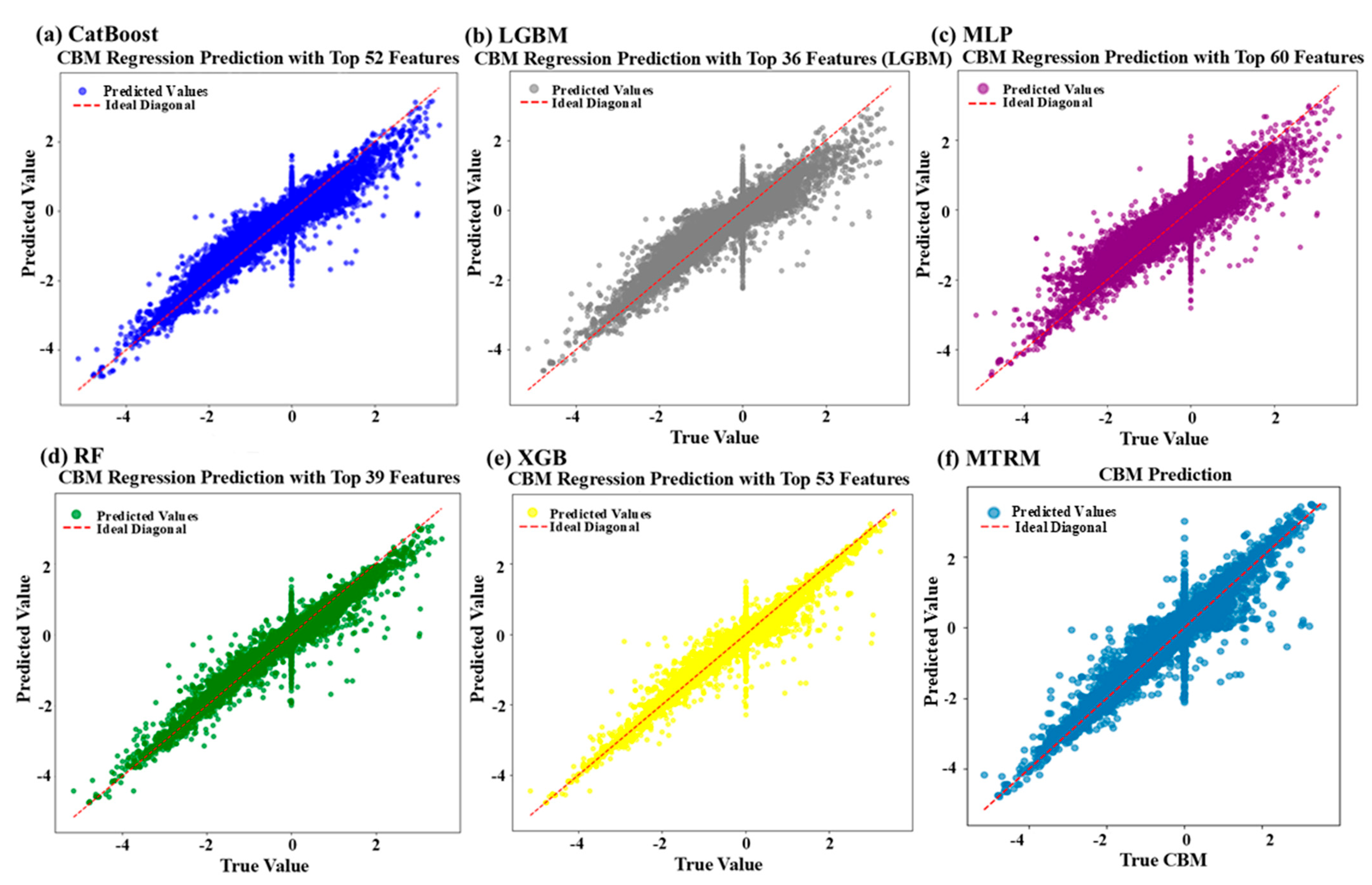
Figure 3 provides scatter plots of predicted versus actual values to visually assess the predictive accuracy of six machine-learning models. The closer the points are to the ideal diagonal line, the higher the prediction accuracy and the lower the error. Despite utilizing only 36 features, the LightGBM model still achieves good predictive performance (R² = 0.7602), demonstrating excellent feature selection and generalization capability. Conversely, the MLP model, despite employing the highest number of features (60), performs the worst (R² = 0.6348, MSE = 0.2762), suggesting that single-task deep learning models struggle in high-dimensional input spaces due to overfitting or the curse of dimensionality.

The proposed multi-task neural network model (MTRM), although slightly inferior in CBM prediction (R² = 0.7313) compared to the top-performing traditional models, maintains stable and reliable predictive capability. The slight reduction in accuracy is a trade-off to achieve multi-task joint optimization. Traditional tree-based models excel in single-task CBM predictions, whereas MTRM is more advantageous in multi-task prediction scenarios.

4.2. Comparison of VBM Prediction Performance

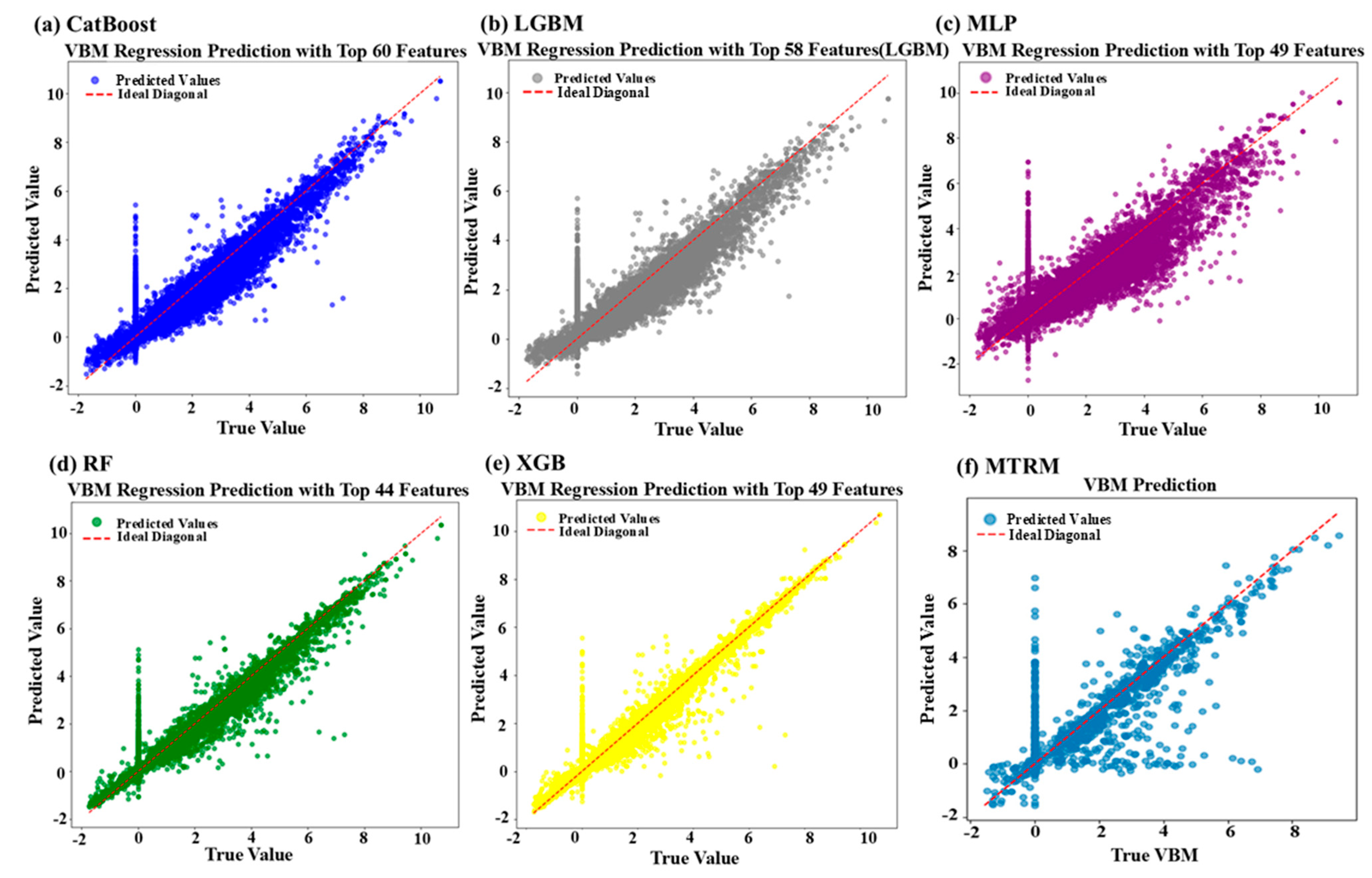
Figure 4 illustrates variations in R² scores for five different machine-learning models at varying feature counts in the test set, with the optimal feature count indicated by a red dashed line. Specifically, the CatBoost model (Figure 4a) achieves its optimal performance at k = 60. The LightGBM model (Figure 4b) performs best at k = 58, while the MLP model (Figure 4c) peaks at k = 49. The Random Forest (RF) model (Figure 4d) reaches peak performance at k = 44 but declines thereafter. The XGBoost model (Figure 4e) achieves optimal results at k = 49.

Table 2. Comparison of Model Performance for VBM Prediction: MSE, RMSE, MAE, and R² Metrics.

Model	MSE	RMSE	MAE	R2
MTRM	0.9055	0.9516	0.4346	0.7300
XGBoost	0.6343	0.7964	0.3954	0.8086
Random Forest	0.6814	0.8254	0.4421	0.7944
MLP	1.0948	1.0463	0.7308	0.6696
CatBoost	0.6128	0.7828	0.4626	0.8150
LightGBM	0.6504	0.8065	0.4968	0.8037

summarizes the regression evaluation metrics for these models.

Scatter plots of predicted versus actual values (Figure 5) demonstrate that CatBoost, XGBoost, and Random Forest predictions are closely clustered around the ideal diagonal line. Specifically, Random Forest and XGBoost exhibit compact and stable error distributions, whereas CatBoost slightly deviates but maintains strong overall performance. Conversely, the MLP and MTRM models perform poorly in extreme value ranges, indicating limitations in capturing complex nonlinear feature interactions. In the VBM prediction task, CatBoost (R² = 0.8150) and XGBoost (R² = 0.8086) achieve the best performance. Although the MTRM model (R² = 0.7327) lags slightly behind, it still exhibits stable predictive capability. The MLP model performs the worst (R² = 0.6696), highlighting difficulties of single neural network architectures in capturing complex feature interactions. Random Forest and LightGBM performance are intermediate yet overall superior to MTRM.

Though not the optimal choice for single-task predictions, MTRM offers enhanced stability and adaptability in multi-task scenarios due to its end-to-end architecture. The excellent performance observed within a feature range of 40–60 underscores the complexity of feature interactions required for accurate VBM predictions, explaining the superior performance of tree-based models.

4.3. Comparison of STH Prediction Performance

In the STH prediction task, the multi-task neural network model (MTRM) significantly outperforms traditional models, as summarized in

Table 3. Comparison of Model Performance for STH Prediction Using Predicted CBM and VBM: MSE, RMSE, MAE, and R² Metrics.

Model	MSE	RMSE	MAE	R2
MTRM	0.0001	0.0076	0.0015	0.8265
XGBoost	0.0002	0.0145	0.0028	0.3614
Random Forest	0.0002	0.0152	0.0029	0.3033
MLP	-	-	-	-
CatBoost	0.0006	0.0242	0.0068	−0.7684
LightGBM	0.0007	0.0259	0.0075	−1.0205

. MTRM achieves remarkably low MSE (0.0001) and RMSE (0.0076), and a very high R² score (0.8265), demonstrating effective joint optimization of CBM, VBM, and STH predictions. This effectively prevents cumulative error propagation common in traditional approaches, significantly enhancing overall prediction accuracy.

In contrast, traditional cascade prediction methods (XGBoost, Random Forest, CatBoost, and LightGBM) perform poorly, exhibiting substantial fluctuations in R², including negative values and significantly higher MSEs. This instability stems from the amplification of prediction errors propagated from initial CBM and VBM predictions into subsequent STH prediction steps. Figure 6 provides scatter plot comparisons of five machine-learning models (CatBoost, LightGBM, RF, XGBoost, and MTRM) for STH prediction; MLP is excluded due to poor performance. Ensemble models (Figure 6a–d) generally show numerous predictions clustered at lower ranges and deviating substantially from the ideal diagonal line, particularly CatBoost and LGBM, which exhibit limited prediction accuracy at higher values. XGBoost and Random Forest predictions slightly improve, but still systematically underestimate. In contrast, MTRM predictions (Figure 6e) are balanced and closely distributed around the ideal line. This visual difference can be attributed to the way each model handles edge cases in the dataset. Approximately 90.33% of STH values are exactly zero, resulting in a highly imbalanced label distribution. Traditional tree-based models tend to overfit this dominant region, leading to horizontal line artifacts in scatter plots. For CBM and VBM, many samples have true values equal to 0 eV, which contributes to vertical lines in scatter plots due to the models’ inability to accurately regress exact zeros. In contrast, MTRM demonstrates greater robustness by leveraging joint task optimization, nonlinear feature representations, and physical constraints (e.g., STH ≥ 0), which help suppress such artifacts and yield more continuous and physically meaningful predictions. Moreover, the MTRM training loss curve (Figure 6f) stabilizes after approximately 50 training epochs, confirming good learning and fitting capabilities. Consequently, MTRM performs superiorly in STH prediction.

Traditional cascading methods independently predict CBM and VBM first, then use these outputs to predict STH, inherently susceptible to cumulative error propagation. Conversely, MTRM’s end-to-end joint training significantly enhances predictive stability and overall accuracy. Furthermore, we adjusted the overpotential conditions: χ (H₂) from the initial 0.2 eV to three levels (0.1 eV, 0.2 eV, 0.3 eV), and χ (O₂) from the initial 0.6 eV to four levels (0.4 eV, 0.5 eV, 0.6 eV, 0.7 eV). The resulting STH values were averaged to form a new dataset. After retraining the MTRM model on this dataset, the predictive results (shown in

Table 4. MSE, RMSE, MAE, and R² for CBM, VBM, and STH predictions based on MTRM under varying overpotential conditions.

	MSE	RMSE	MAE	R2
CBM	0.1924	0.4387	0.2357	0.7502
VBM	0.8672	0.9312	0.4391	0.7415
STH	0.0001	0.0081	0.0016	0.8251

) demonstrate similar high performance as previously achieved under the fixed overpotential conditions (0.2 eV, 0.6 eV), confirming the robustness of the proposed model.

5. Conclusions

The potential of a multi-task regression model (MTRM) has been demonstrated in predicting the photocatalytic performance of inorganic materials, specifically focusing on the conduction band minimum (CBM), valence band maximum (VBM), and solar-to-hydrogen efficiency (STH). The proposed model efficiently integrates machine-learning techniques to predict these critical parameters simultaneously, addressing the issue of error propagation commonly seen in traditional cascading prediction models. Our results indicate that while single-task tree-based models like Random Forest and CatBoost perform well individually for CBM and VBM prediction, the MTRM excels in a multi-task setting. Notably, for STH prediction, the MTRM outperforms traditional methods, achieving an exceptionally low MSE of 0.0001 and a high R² of 0.8265. This demonstrates the power of multi-task learning in improving overall prediction stability and generalization, especially when predicting multiple interrelated tasks like CBM, VBM, and STH. The key advantage of the MTRM lies in its end-to-end optimization, where the model jointly optimizes all three tasks, reducing the error propagation and enhancing the final predictions. This approach provides a more robust and reliable framework for predicting photocatalytic material performance, offering a promising avenue for accelerating the design and screening of efficient photocatalysts for hydrogen production. Overall, this study underscores the potential of applying advanced machine-learning techniques in the field of materials science, particularly in renewable energy research.