
Poisoning Effect of CO: How It Changes Hydrogen Electrode Reaction and How to Analyze It Using Differential Polarization Curve

Abstract
:1. Introduction
2. Results
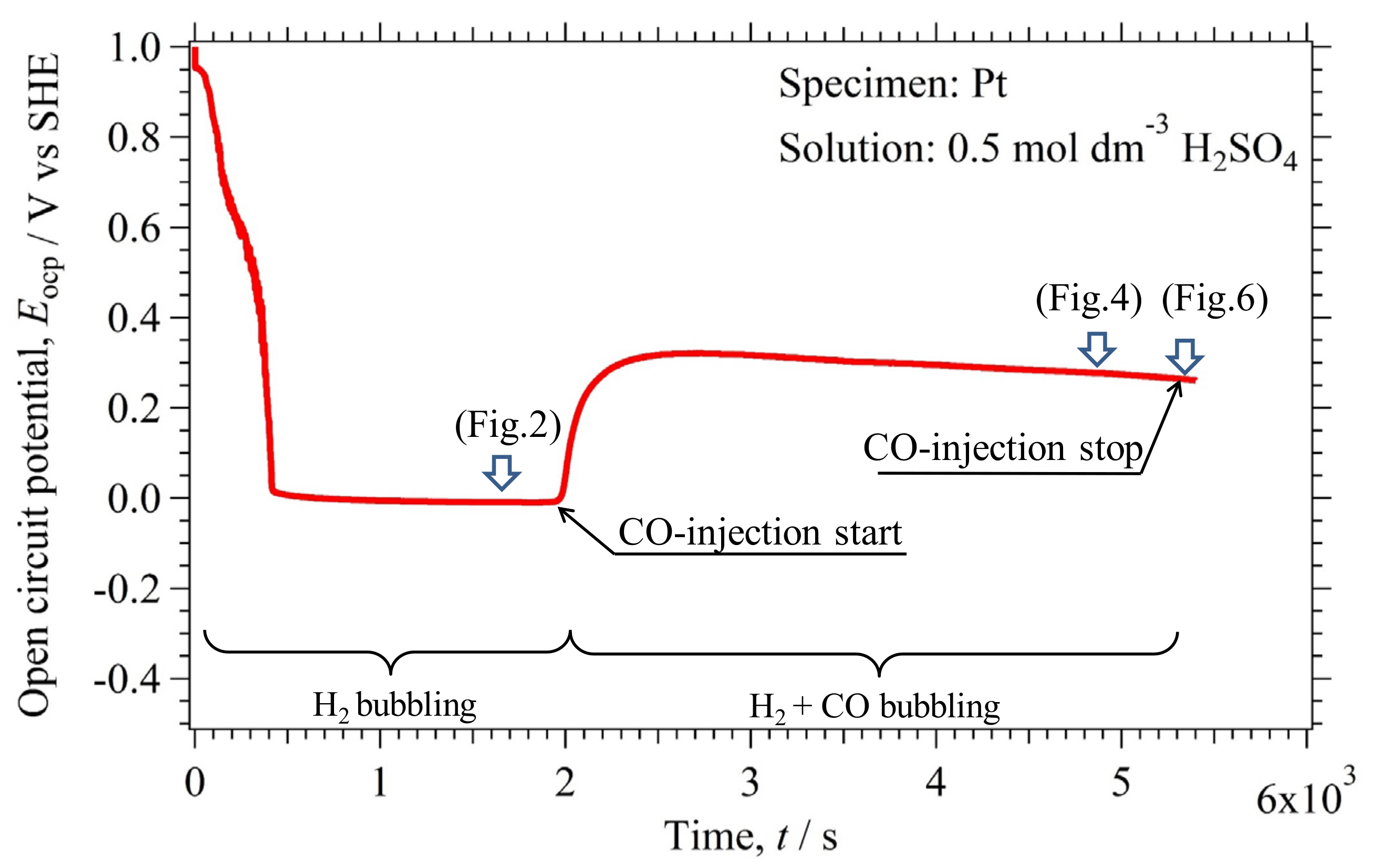
2.1. Variation of the Open Circuit Potential with Time
2.2. and
2.2.1. and in the Environment (I)
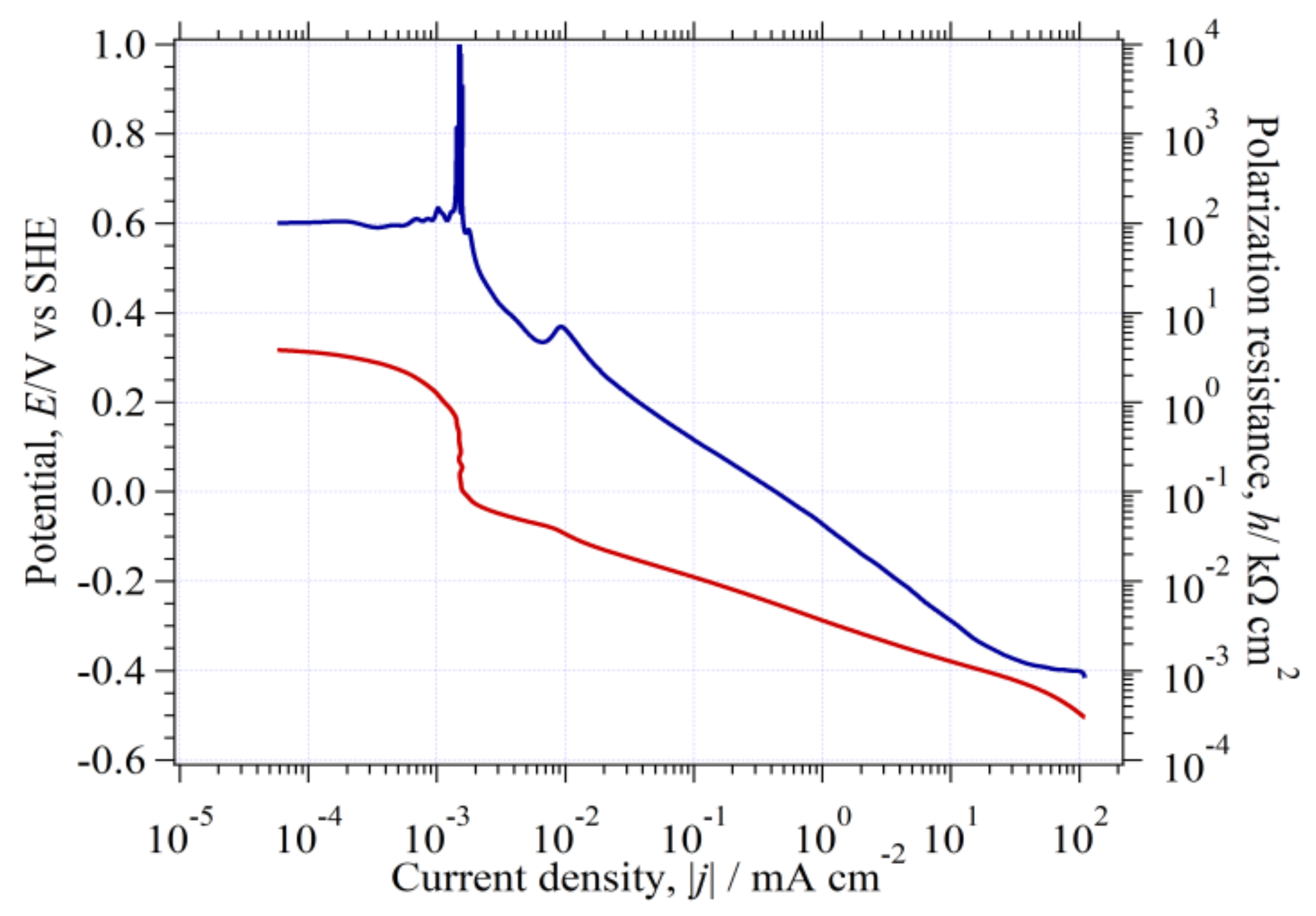
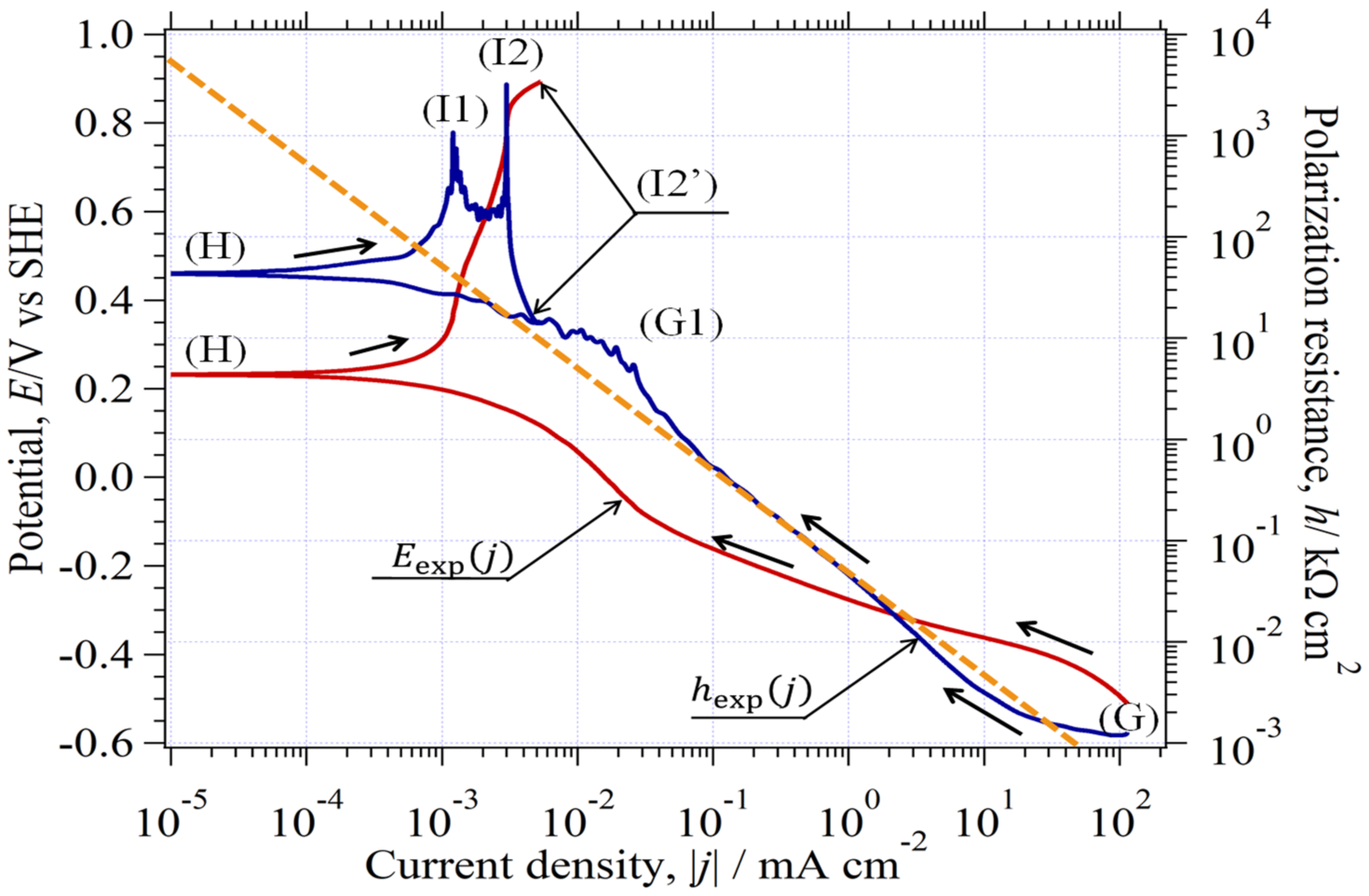
2.2.2. and in the Environment (II)
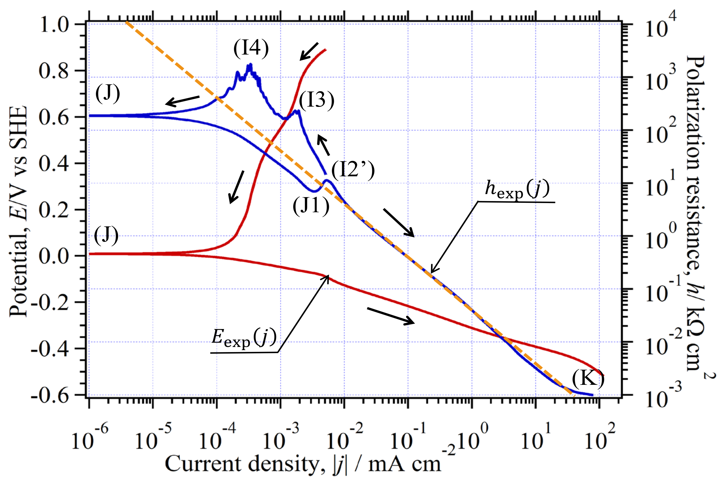
2.2.3. and in the Environment (III)
3. Discussion
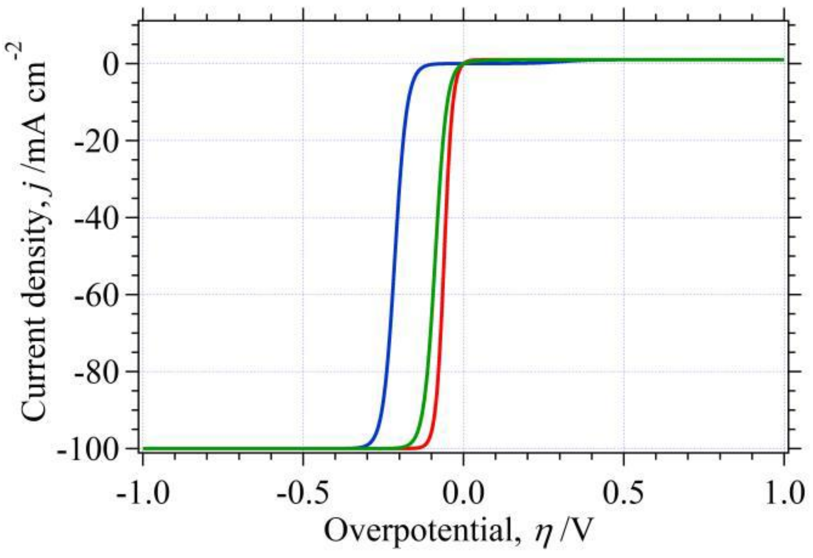
3.1. Single Electrode Reaction and Its Classification
- (A)
- Reversible reaction; ;
- (B)
- Irreversible reaction; ;
- (C)
- Quasireversible reaction; .
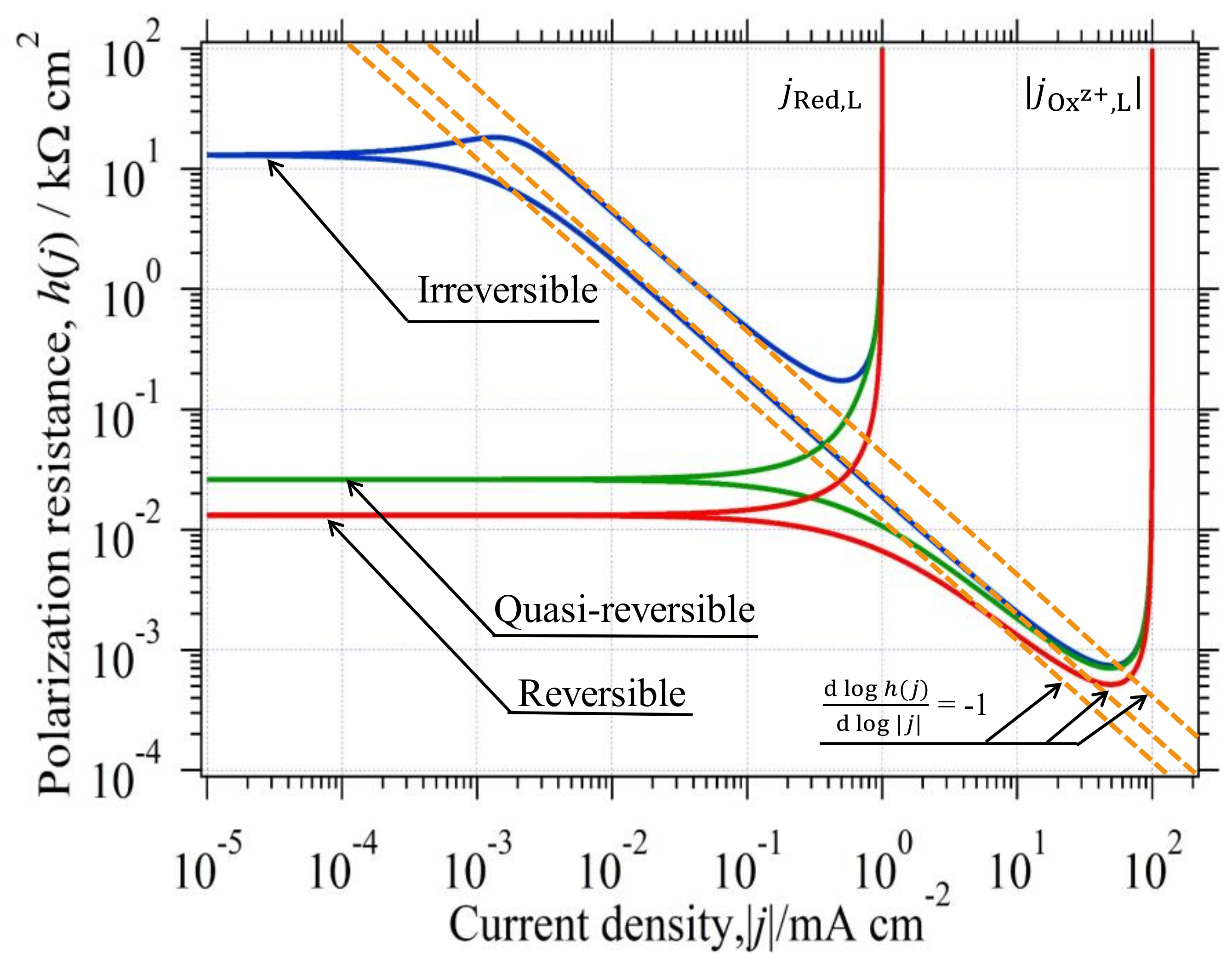
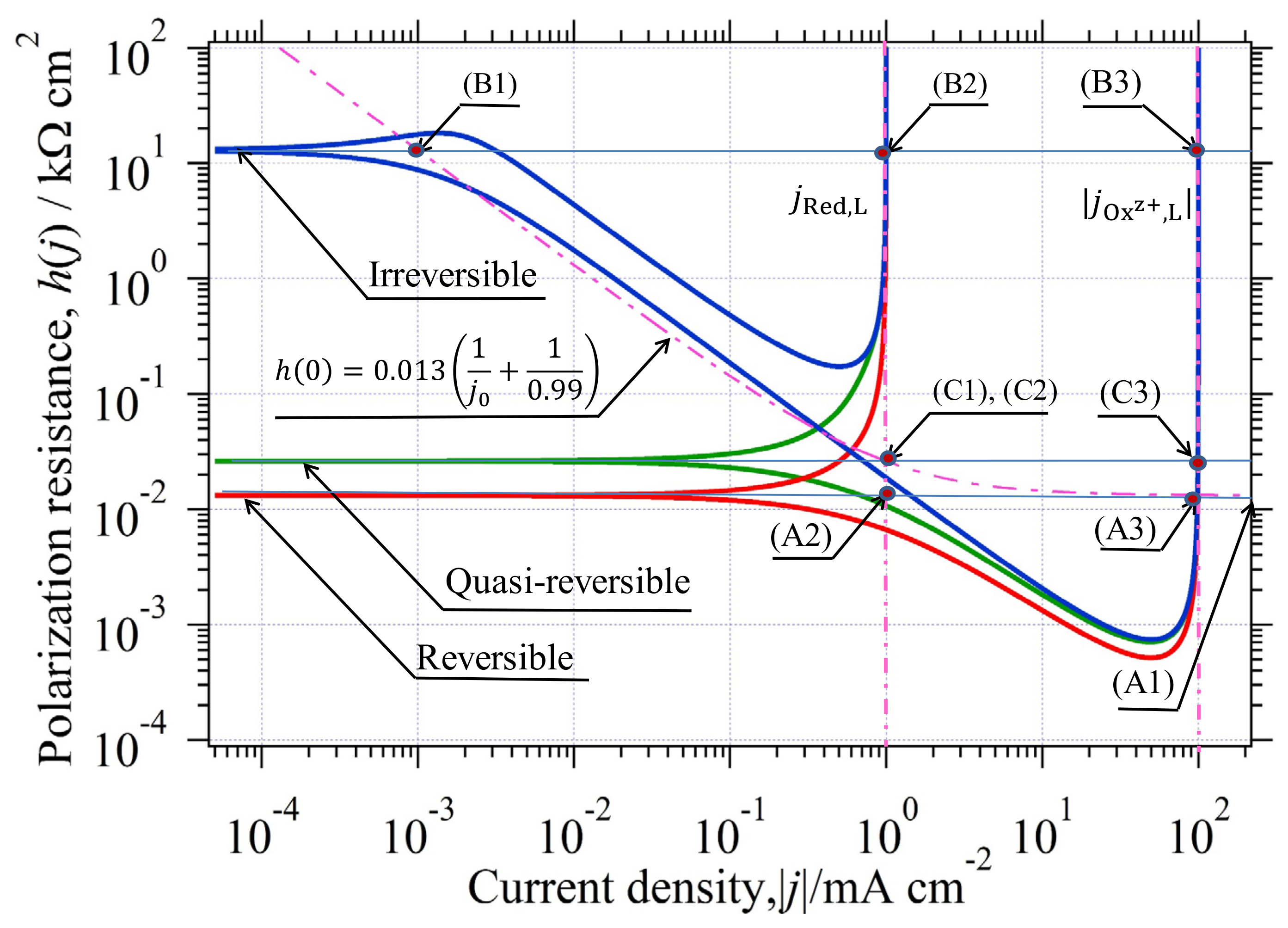
3.2. Single Electrode Reaction and Its Polarization Resistance
3.3. The Relationship between the Tafel Extrapolation Method (tem) and H(j)
3.4. Kinetic Parameter Determination Using
3.4.1. Reversible Reaction
3.4.2. Irreversible Reaction
3.4.3. Quasireversible Reaction
3.5. Graphical Determination of
3.6. Physical Factors Influenced on
3.6.1. Effective Area of Electrode
3.6.2. Solution Resistance
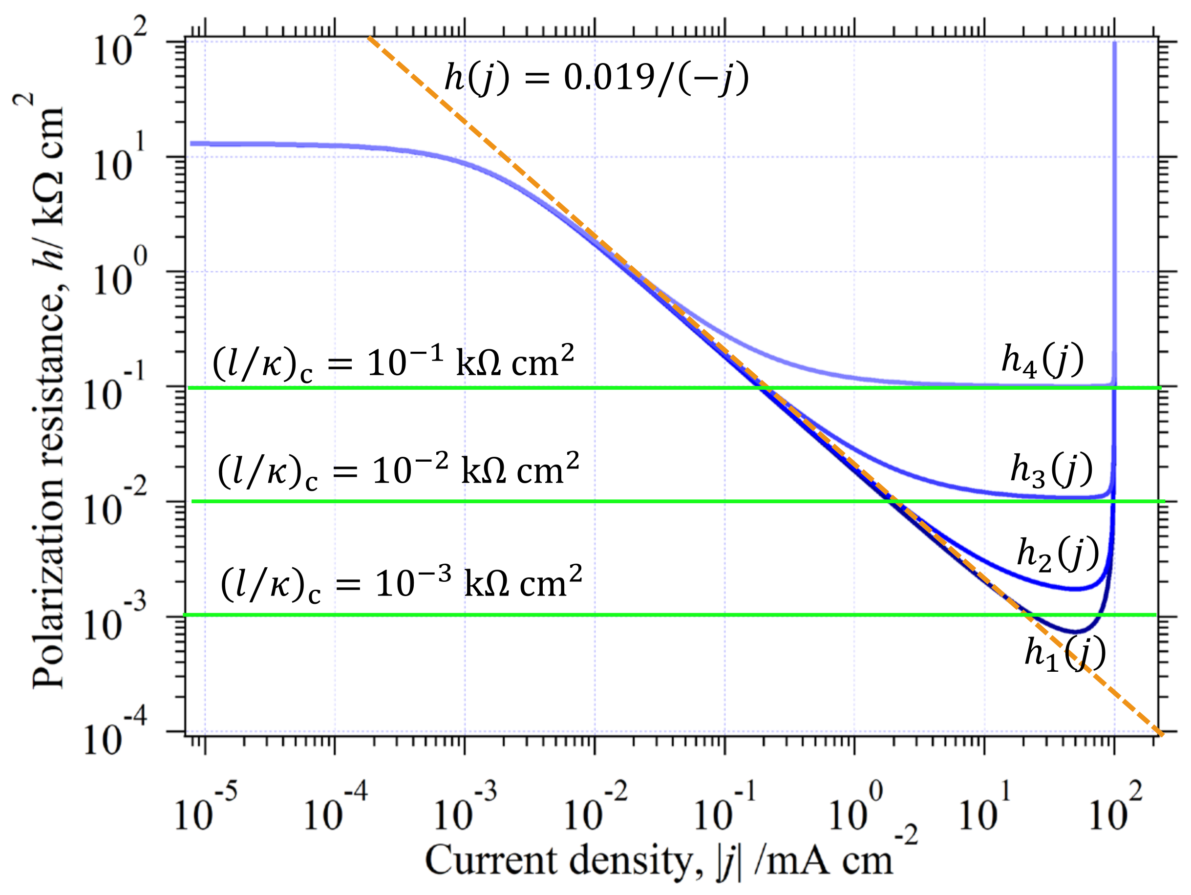
3.6.3. The in the Whole Current Range
3.7. Determination of Stable Chemical Species on Using E-pH Diagram
3.8. Curve Analysis for Reversible HER in Environment (I)
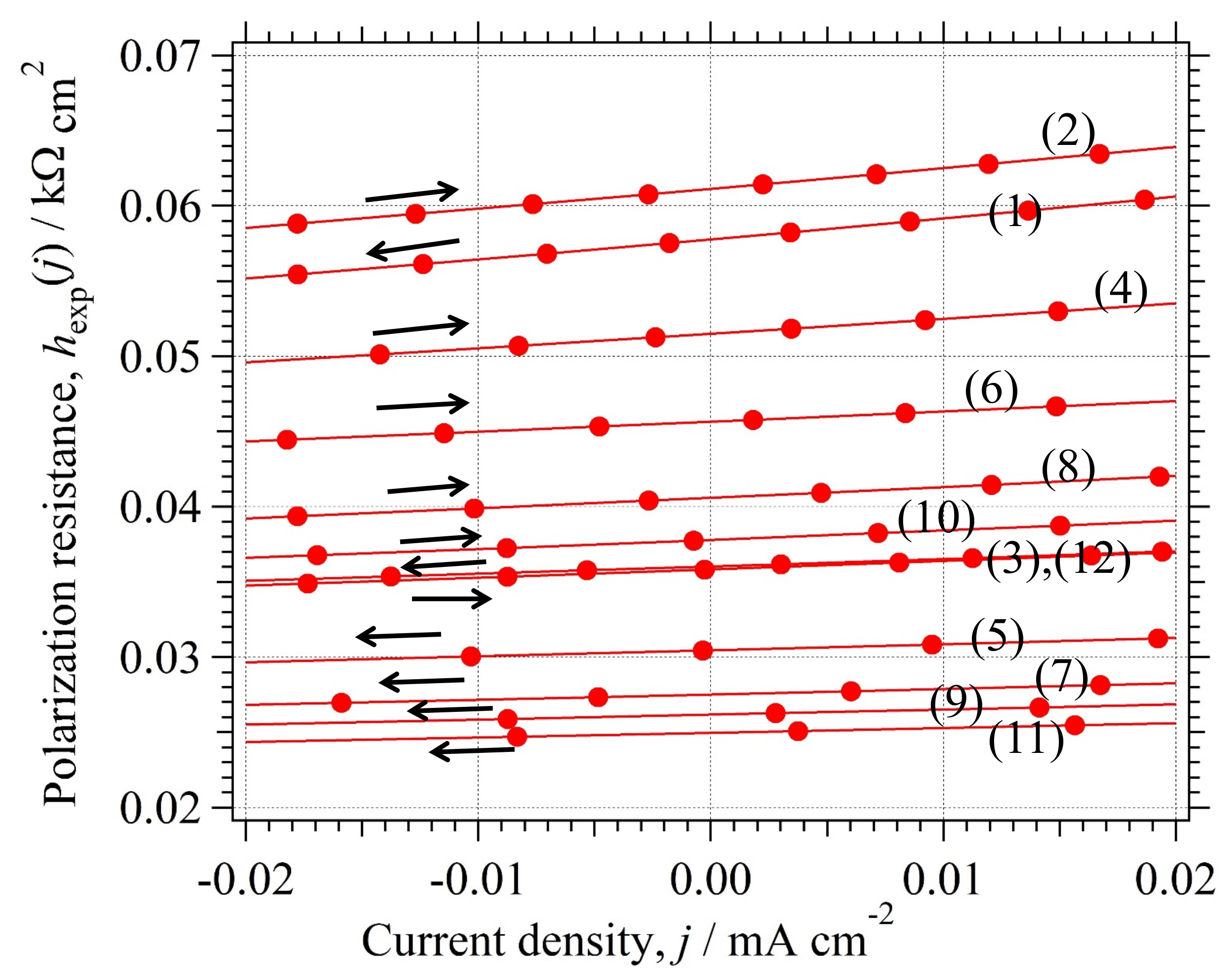
3.8.1. Estimation of and
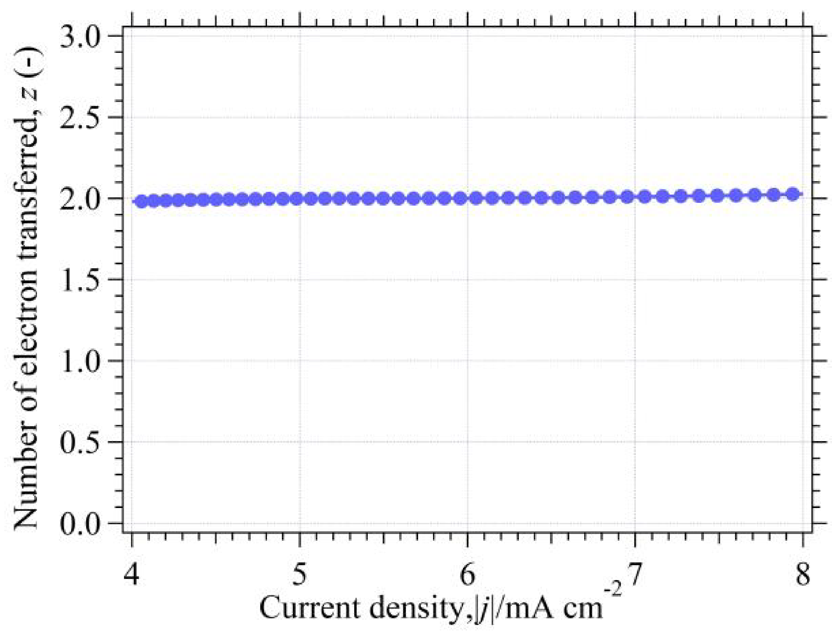
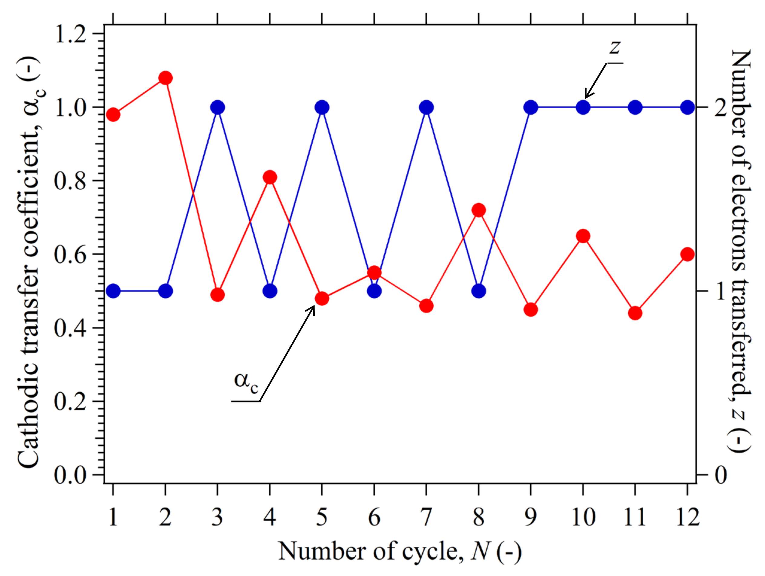
3.8.2. Determination of z for Reversible HER
3.8.3. Confirmation of for Reversible HER
3.8.4. Determination of Kinetic Parameters for Reversible HER
3.8.5. Agreement between and
3.9. Curve Analysis of in Environment (II)
3.9.1. Analysis of
- (a)
- Point Analysis of
- (b)
- Part analysis of
- (b1)
- Part Analysis of
- (b2)
- Part analysis of
- (b3)
- Part analysis of
3.9.2. Analysis of
- (a)
- Part analysis of
- (b)
- Analysis of
- (c)
- Analysis of
- (d)
- Analysis of
3.9.3. Analysis of
- (a)
- Part analysis of
- (b)
- Part analysis of
- (c)
- Part analysis of
- (d)
- Part analysis of
3.10. Analysis of Quasireversible HER (Environment (III))
3.10.1. Estimation of at CO Stopped
3.10.2. Determination of Kinetic Parameters in the CO-Stopped Solution
3.10.3. Graphical Determination of jA(0)
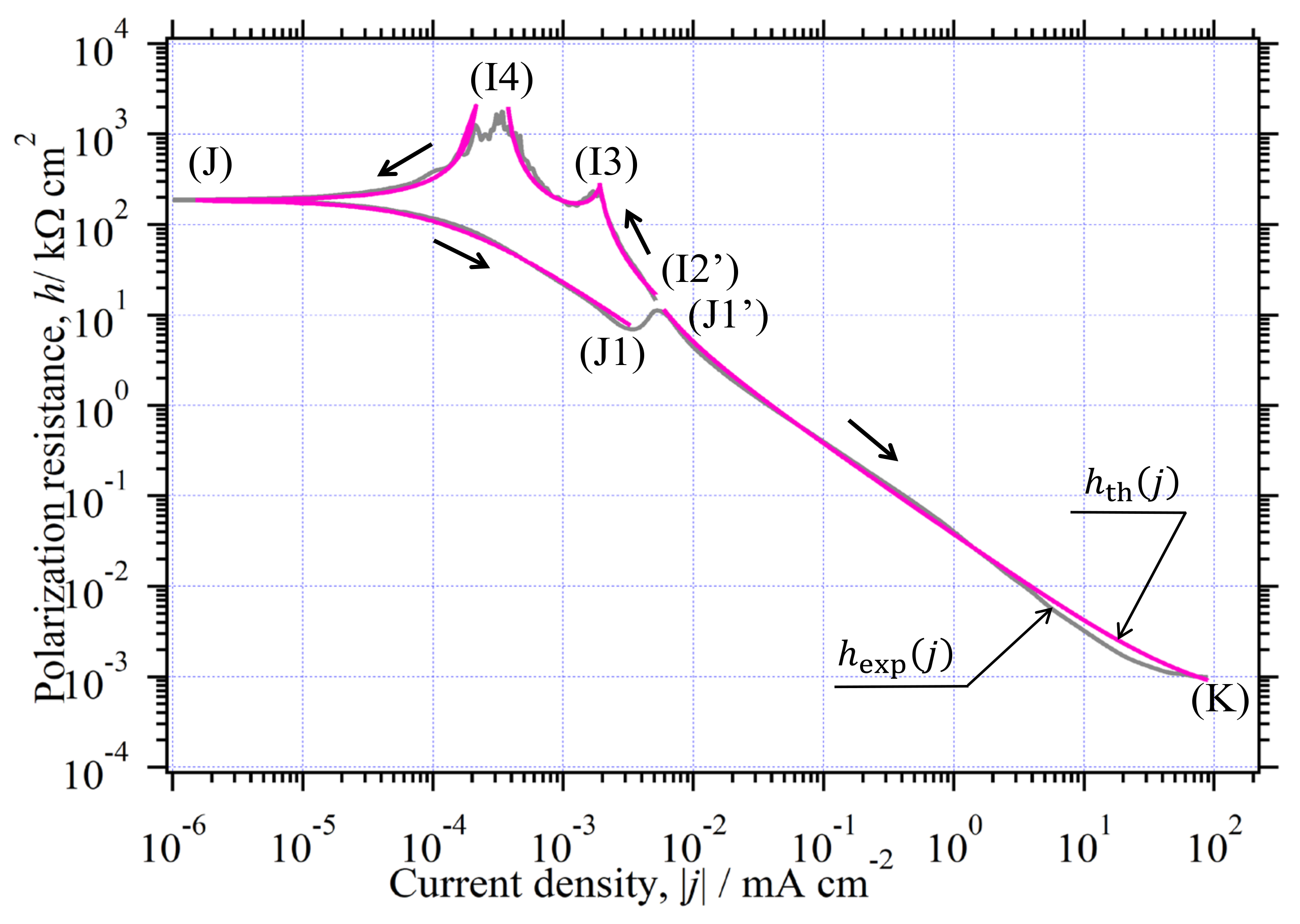
3.10.4. Agreement between Eexp(j) and Eth(j)
- (1)
- (2)
- (3)
4. Experimental Section
4.1. Specimens
4.2. Test Solution
4.3. Measurements
5. Conclusions
Author Contributions
Funding
Conflicts of Interest
Appendix A. List of Symbols
- is the net current as a function of overpotential (mA).
- is the anodic branch current as a function of overpotential (mA).
- is the cathodic branch current as a function of overpotential (mA).
- S is the geometrical surface of electrode (cm2).
- is the effective area where the flows (cm2).
- is the effective area where the flows (cm2).
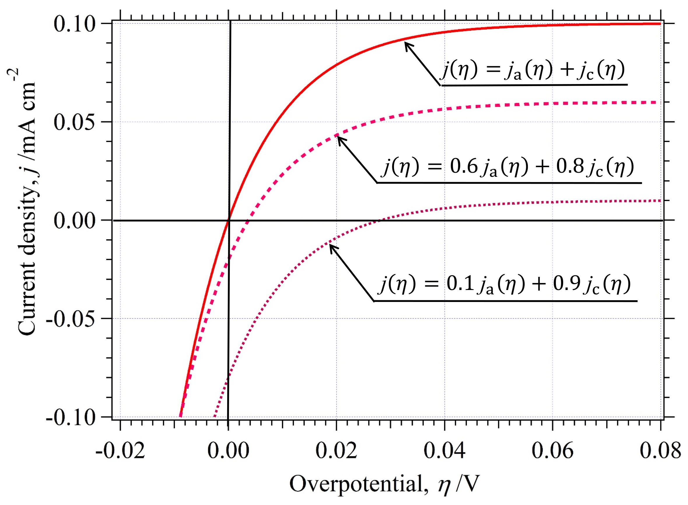
- is the weighting factor that has suitably weighted value in proportion to the surface of the anode (-).
- is the weighting factor that has suitably weighted value in proportion to the surface of the cathode (-).
- j(η) is the net current density as a function of overpotential (mA cm−2).
- is the anodic branch current density as a function of overpotential (mA cm−2).
- is the cathodic branch current density as a function of overpotential (mA cm−2).
- is the minimum in the state of (mA cm−2).
- is the maximum in the state of (mA cm−2).
- η is the overpotential between an applied potential, E and the (V).
- (A1).
- is the equilibrium electrode potential (V vs. SHE).
- (A2).
- is the standard electrode potential (V vs. SHE).
- is the formal electrode potential (V vs. SHE).
- z is the number of electrons transferred (-).
- F is the Faraday’s constant ().
- R is the gas constant .
- T is the absolute temperature (K).
- is the activity of reductant (Red) in the bulk solution (-).
- is the activity of oxidant () in the bulk solution (-).
- is the concentration of the Red in the bulk solution ().
- is the concentration of the in the bulk solution ().
- fa is F/RT (V−1).
- fc is F/RT (V−1).
- is the anodic transfer coefficient (-).
- is the cathodic transfer coefficient (-) ().
- f is z F/RT (V−1).
- f = fa + fc = z F/RT (V−1) (A3).
- is the limiting diffusion current density of the Red, .
- (A4)
- is the limiting diffusion current density of the , .
- (A5).
- is a diffusion coefficient of the Red (cm2 s−1).
- is a diffusion coefficient of the (cm2 s−1).
- is the Nernst diffusion layer thickness concerning the Red (cm).
- is the Nernst diffusion layer thickness concerning the (cm).
- is the rate constant of the Red (cm s−1).
- is the rate constant of the (cm s−1).
- is the total exchange current density .
- is the exchange current density for charge transfer process .
- (A6).
- is the standard heterogeneous rate constant (cm s−1).
- is the polarization resistance relating to oxide film or product layer ().
- is the thickness of oxide film or product layer (cm).
- is the conductivity of oxide film or product layer ().
- is the polarization resistance relating to solution ().
- is the distance between the anodic site and the cathodic site (cm).
- is the conductivity of the solution ().
References
- Takahashi, M.; Masuko, N. Kogyodenkai-No-Kagaku; AGNE: Tokyo, Japan, 1979; pp. 181–192. [Google Scholar]
- Haruyama, S. Hyomengijyutusha-Notameno-Denkikagaku, 2nd ed.; Maruzen: Tokyo, Japan, 2005; pp. 65–86; 88–90. [Google Scholar]
- Bard, A.J. (Ed.) Hydrogen Encyclopedia of Electrochemistry of the Elements; Marcel Dekker: New York, NY, USA, 1969; Volume IXa, pp. 384–592. [Google Scholar]
- Adams, R.N. Electrochemistry at Solid Electrodes; Marcel Dekker: New York, NY, USA, 1969; pp. 187–212. [Google Scholar]
- Charlot, G.; Badoz-Lambling, J.; Tremillon, B. Les Reactions Electrochimiques; Droits d’Auteur, Masson: Paris, France, 1959; pp. 13–26; 41–83. (In Japanese) [Google Scholar]
- Rieger, P.H. Electrochemistry, 2nd ed.; Chapman & Hill: New York, NY, USA, 1994; pp. 151–164; 334–337. [Google Scholar]
- Gileadi, E. Physical Electrochemistry; Wiley-VCH: Weinheim, Germany, 2011; pp. 99–112; 195–204. [Google Scholar]
- Bard, A.J.; Faulkner, L.R. Electrochemical Methods, 2nd ed.; John Wiley & Sons: New York, NY, USA, 1980; pp. 1–43. [Google Scholar]
- Brteiter, M.W. Electrochemical Processes in Fuel Cell; Springer: Berlin, Germany, 1969; pp. 1–184. [Google Scholar]
- Bokris, J.O.; Ready, A.K. Modern Electrochemistry; Plenum Press: New York, NY, USA, 1983; Volume 1 and 2, pp. 1231–1250. [Google Scholar]
- Bortoloti, F.; Garcia, A.C.; Angelo, A.C.D. Electronic effect in intermetallic electrocatalysts with low susceptibility to CO poisoning during hydrogen oxidation. Int. J. Hydrogen Energy 2015, 401, 10816–10824. [Google Scholar] [CrossRef]
- Luque, G.C.; de Chialvo, M.R.G.; Chialvo, A.C. Kinetic Study of the Formic Acid Oxidation on Steady State Using a Flow Cell. J. Solid State Electrochem. 2017, 20, 1209–1217. [Google Scholar] [CrossRef]
- Marozzi, C.A.; de Chialvo, M.R.G.; Chialvo, A.C. Criteria for the selection of the scan rate in the evaluation of the kinetic parameters of the hydrogen oxidation reaction by a potentiodynamic sweep. J. Electroanal. Chem. 2015, 748, 61–69. [Google Scholar] [CrossRef]
- Rau, M.S.; de Chialvo, M.R.G.; Chialvo, A.C. Resolution of the mechanism of CO electrooxidation on steady state and evaluation of the kinetic parameters for Pt and Ru electrodes. J. Solid State Electrochem. 2012, 16, 1893–1900. [Google Scholar] [CrossRef]
- Quaino, P.M.; de Chialvo, M.R.G.; Chialvo, A.C. Hydrogen electrode reaction: A complete kinetic description. Electrochim. Acta 2007, 52, 7396–7403. [Google Scholar] [CrossRef]
- Marozzi, C.A.; Canto, M.R.; Costanza, V.; Chialvo, A.C. Analysis of the use of voltammetric results as a steady state approximation to evaluate kinetic parameters of the hydrogen evolution reaction. Electrochim. Acta 2005, 51, 731–738. [Google Scholar] [CrossRef]
- De Chialvo, M.R.G.; Chialvo, A.C. Hydrogen diffusion effects on the kinetics of the hydrogen electrode reaction. Part I. Theoretical aspects. Phys. Chem. Chem. Phys. 2004, 6, 4009–4017. [Google Scholar] [CrossRef]
- Quaino, P.M.; de Chialvo, M.R.G.; Chialvo, A.C. Hydrogen diffusion effects on the kinetics of the hydrogen electrode reaction Part II. Evaluation of kinetic parameters. Phys. Chem. Chem. Phys. 2004, 6, 4450–4455. [Google Scholar] [CrossRef]
- Fernandez, J.L.; de Chialvo, M.R.G.; Chialvo, A.C. Evaluation of the kinetic parameters of the hydrogen electrode reaction from the analysis of the equilibrium polarisation resistance. Phys. Chem. Chem. Phys. 2003, 5, 2875–2880. [Google Scholar] [CrossRef]
- De Chialvo, M.R.G.; Chialvo, A.C. The Tafel–Heyrovsky route in the kinetic mechanism of the hydrogen evolution reaction. Electrochem. Commun. 1999, 1, 379–382. [Google Scholar] [CrossRef]
- De Chialvo, M.R.G.; Chialvo, A.C. The polarisation resistance, exchange current density and stoichiometric number for the hydrogen evolution reaction: Theoretical aspects. J. Electroanal. Chem. 1996, 415, 97–106. [Google Scholar] [CrossRef]
- De Chialvo, M.R.G.; Chialvo, A.C. Hydrogen evolution reaction: Analysis of the Volmer-Heyrovsky-Tafel mechanism with a generalized adsorption model. J. Electroanal. Chem. 1994, 372, 209–223. [Google Scholar] [CrossRef]
- Seri, O.; Itoh, Y. Differentiating polarization curve technique for determining the exchange current density of hydrogen electrode reaction. Electrochim. Acta 2016, 218, 345–355. [Google Scholar] [CrossRef] [Green Version]
- Seri, O.; Siree, B. The differentiating polarization curve technique for the Tafel parameter estimation. Catalysts 2017, 39, 1–15. [Google Scholar] [CrossRef]
- Seri, O. Differentiating approach to the Tafel slope of hydrogen evolution reaction on nickel electrode. Electrochem. Commun. 2017, 81, 150–153. [Google Scholar] [CrossRef]
- Seri, O. Kinetic parameter determination of ferri/ferrocyanide redox reaction using differentiating polarization curve technique. Electrochim. Acta 2019, 323, 134776–134784. [Google Scholar] [CrossRef]
- Antropov, L.I. Theoretical Electrochemistry; MIR: New York, NY, USA, 1972; p. 393. [Google Scholar]
- Pearson, J.M. “Null” Methods Applied to Corrosion Measurements. Trans. Electrochem. Soc. 1942, 81, 484–510. [Google Scholar] [CrossRef]
- West, J.M. Basic Corrosion and Oxidation, 2nd ed.; Ellis Horwood Ltd.: Chichester, UK, 1980; pp. 103–113. [Google Scholar]
- Pourbaix, M. Atlas of Electrochemical Equilibria; Pergamon Press: New York, NY, USA, 1966; pp. 449–457. [Google Scholar]
- Masuko, N.; Takahashi, M. Denkikagaku; AGNE: Tokyo, Japan, 1993; pp. 43–56. [Google Scholar]
- Nihon, K. (Ed.) Kagakubinran, Kisohen II, 4th ed.; Marzen: Tokyo, Japan, 1993; pp. II156–II160. [Google Scholar]
- Kita, H.; Ye, S.; Aramata, A. Reaction route of hydrogen electrode reaction on platinum. Denki Kagaku Oyobi Kogyo Butsuri Kagaku 1990, 58, 41–44. [Google Scholar] [CrossRef]
- Tang, D.; Lu, J.; Zhuang, L.; Lin, P. Calculations of the exchange current density for hydrogen electrode reactions: A short review and a new equation. J. Electroanal. Chem. 2010, 644, 144–146. [Google Scholar] [CrossRef]
- Mills, I.; Homann, K.; Kallay, N.; Kuchitsu, K. Quantities, Units and Symbols in Physical Chemistry; Blackwell Scientific Publication: Oxford, UK, 1988; p. 109. (In Japanese) [Google Scholar]
- McGlashan, M.L. Physicochemical Quantities and Units, 2nd ed.; The Royal Institute of Chemistry: London, UK, 1971; p. 46. (In Japanese) [Google Scholar]


| Item | Reading | Remarks |
|---|---|---|
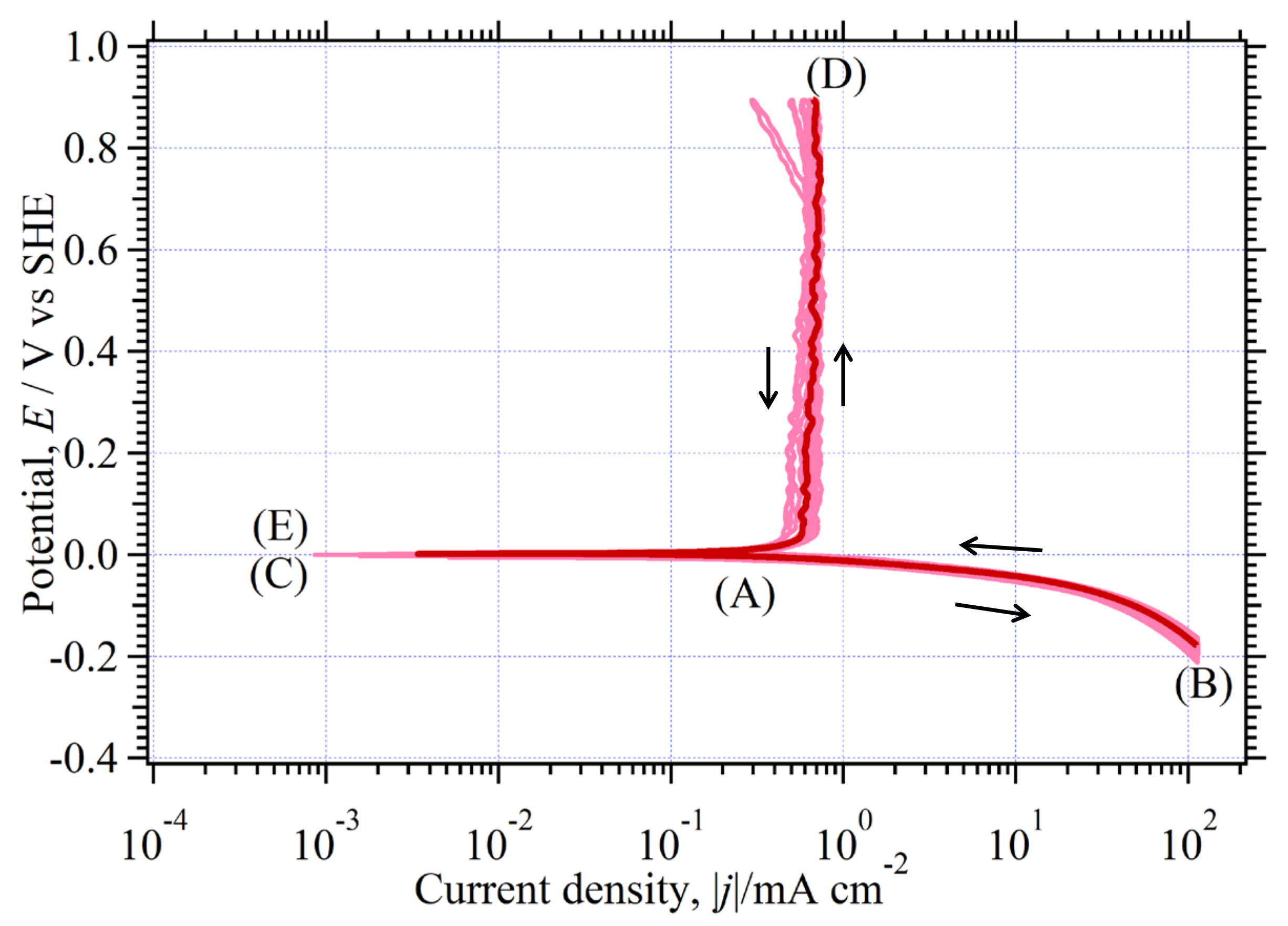
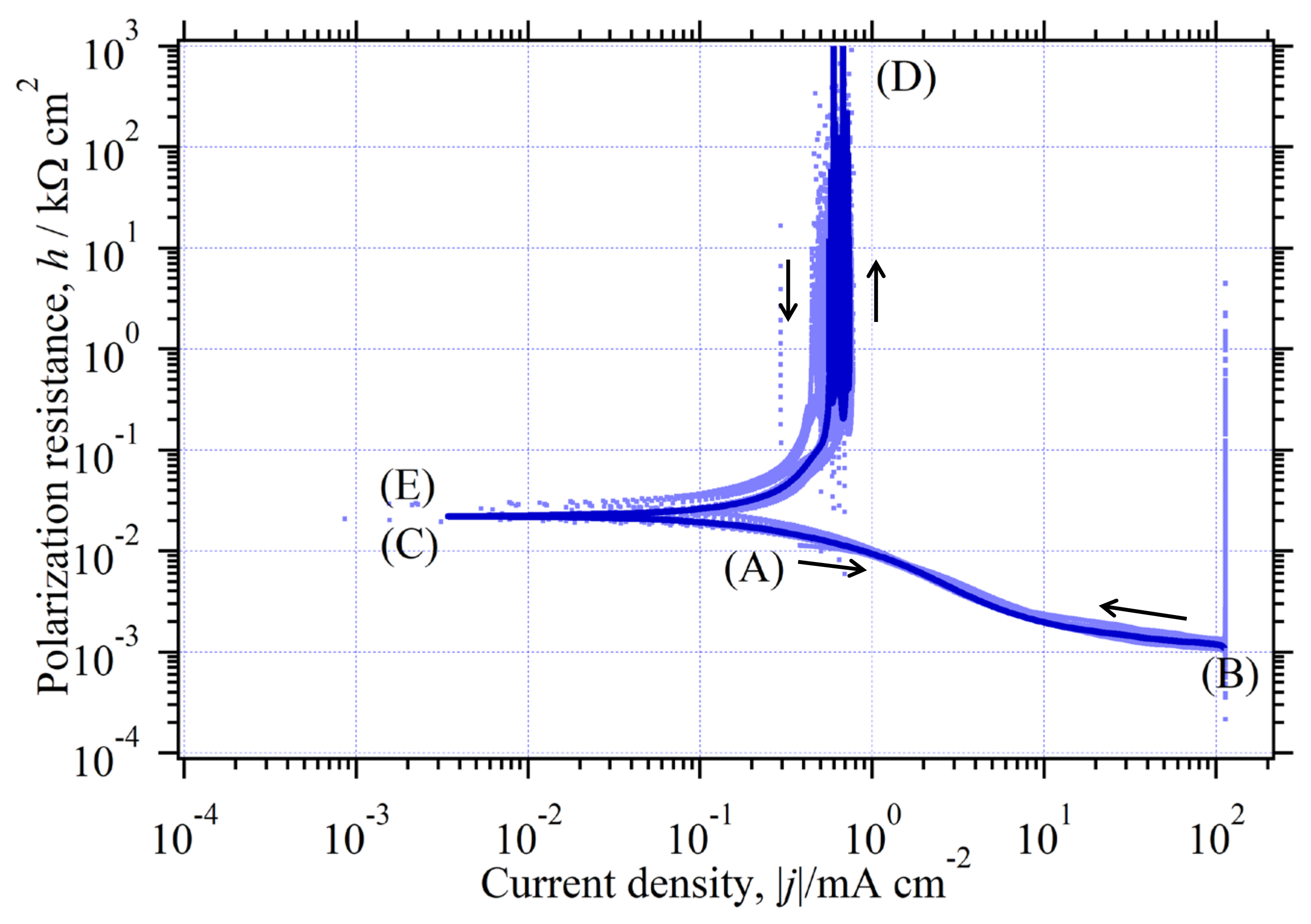
| 0 | (C) and (E) in Figure 2 | |
| (C) and (E) in Figure 3, | ||
| we cannot observe it in Figure 3 | ||
| vertical line having (D) in Figure 2 and Figure 3 | ||
| asymptotic horizontal line; (B) in Figure 3 |
| Item | Reading | Remarks |
|---|---|---|
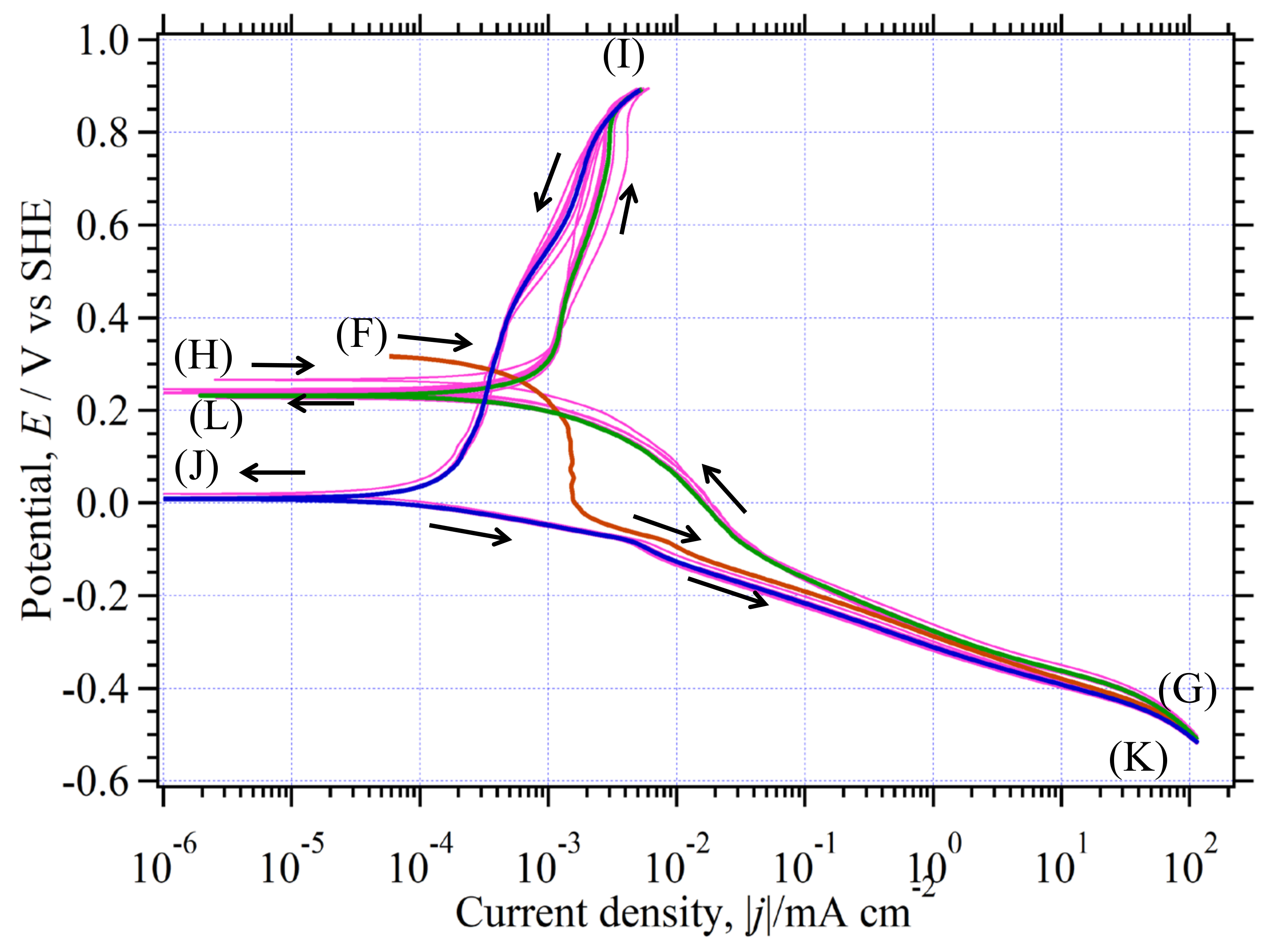
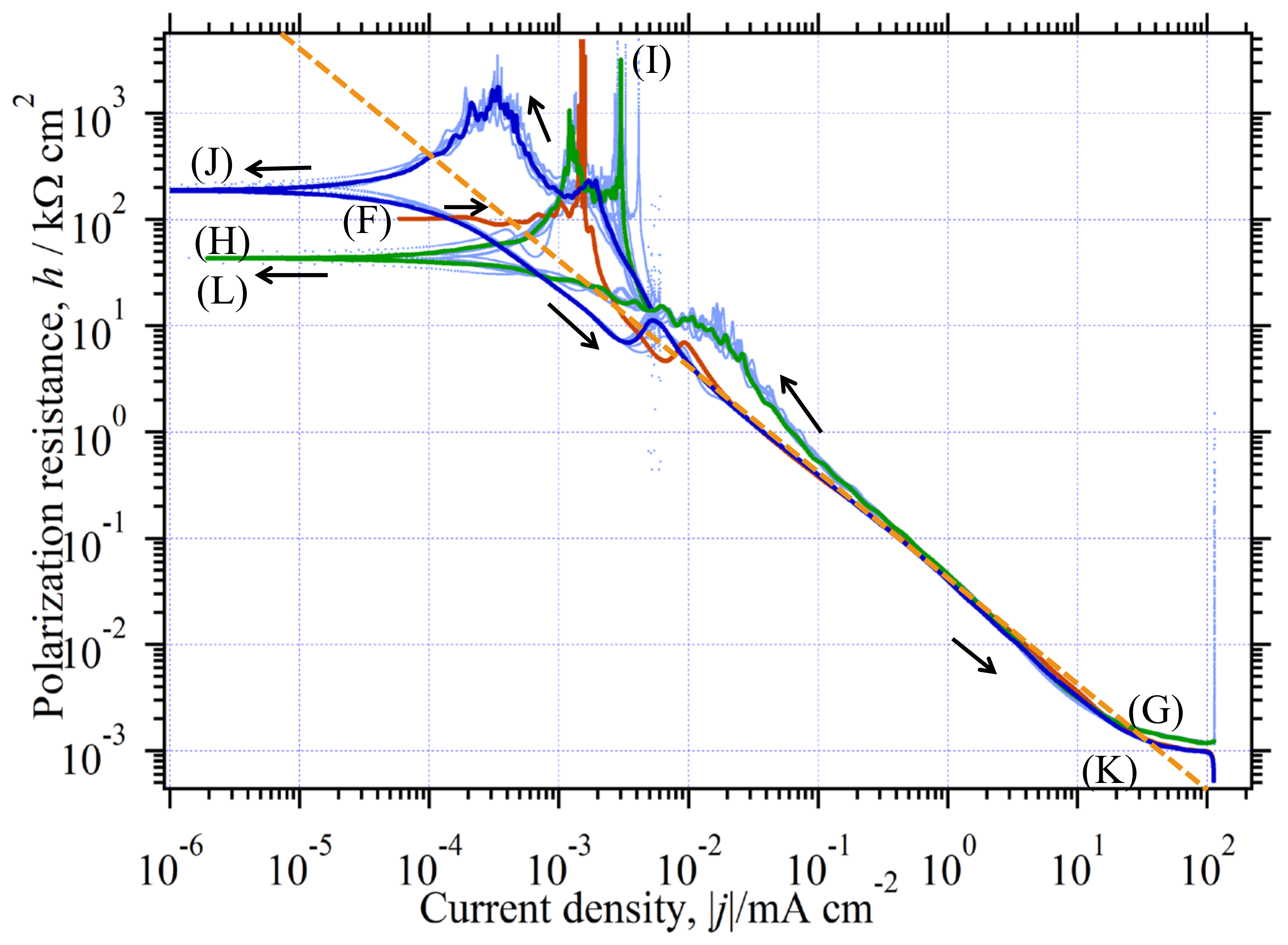
| 0.24 | (H) or (L) in Figure 4 | |
| 0.02 | (J) in Figure 4 | |
| (H) or (L) in Figure 5 | ||
| (J) in Figure 5 | ||
| we cannot observe it in Figure 5 | ||
| red vertical line in Figure 5 | ||
| green vertical line in Figure 5 | ||
| green vertical line in Figure 5 | ||
| asymptotic line; (G) or (K) in Figure 5 |
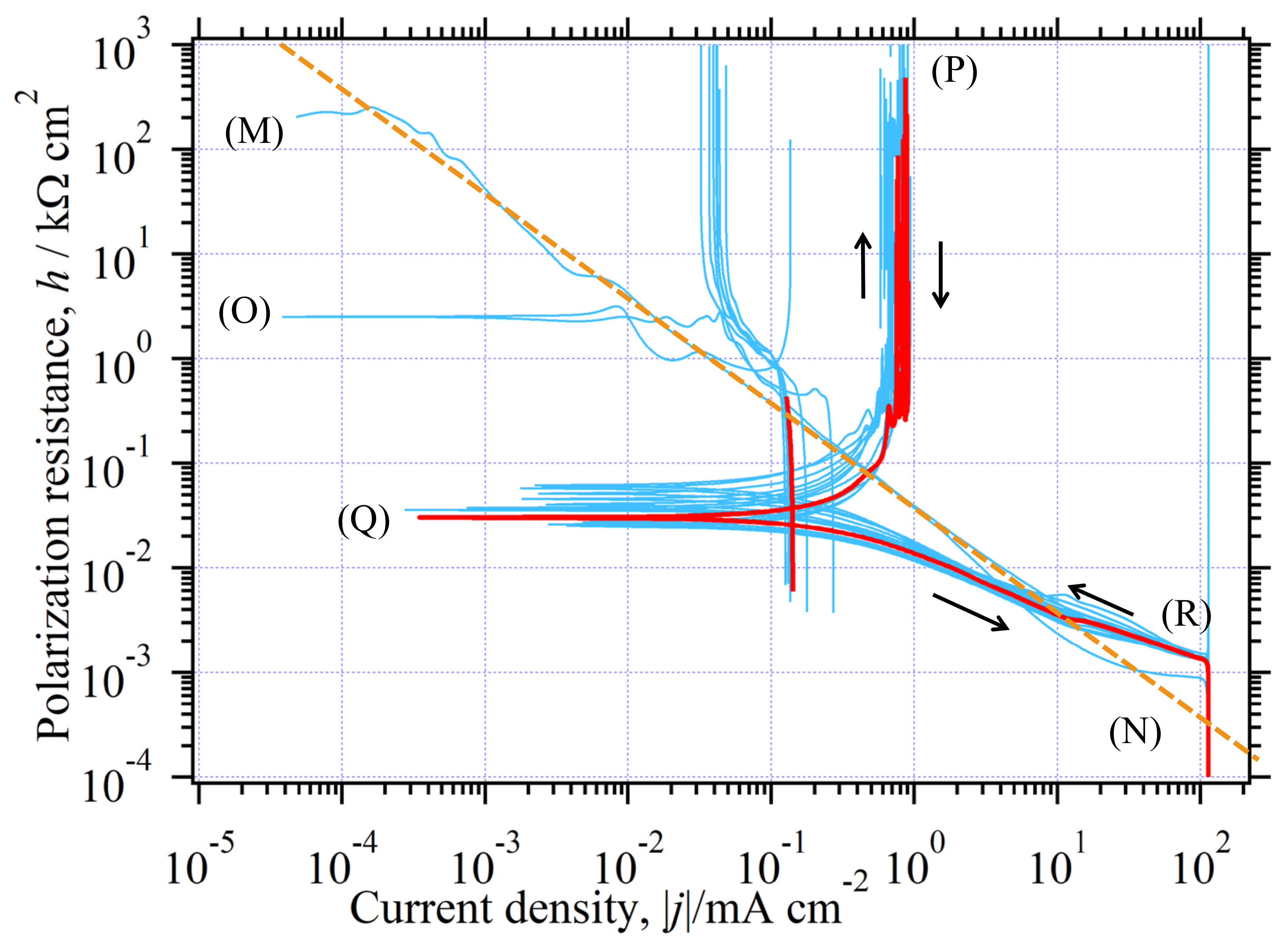
| Item | Reading | Remarks |
|---|---|---|
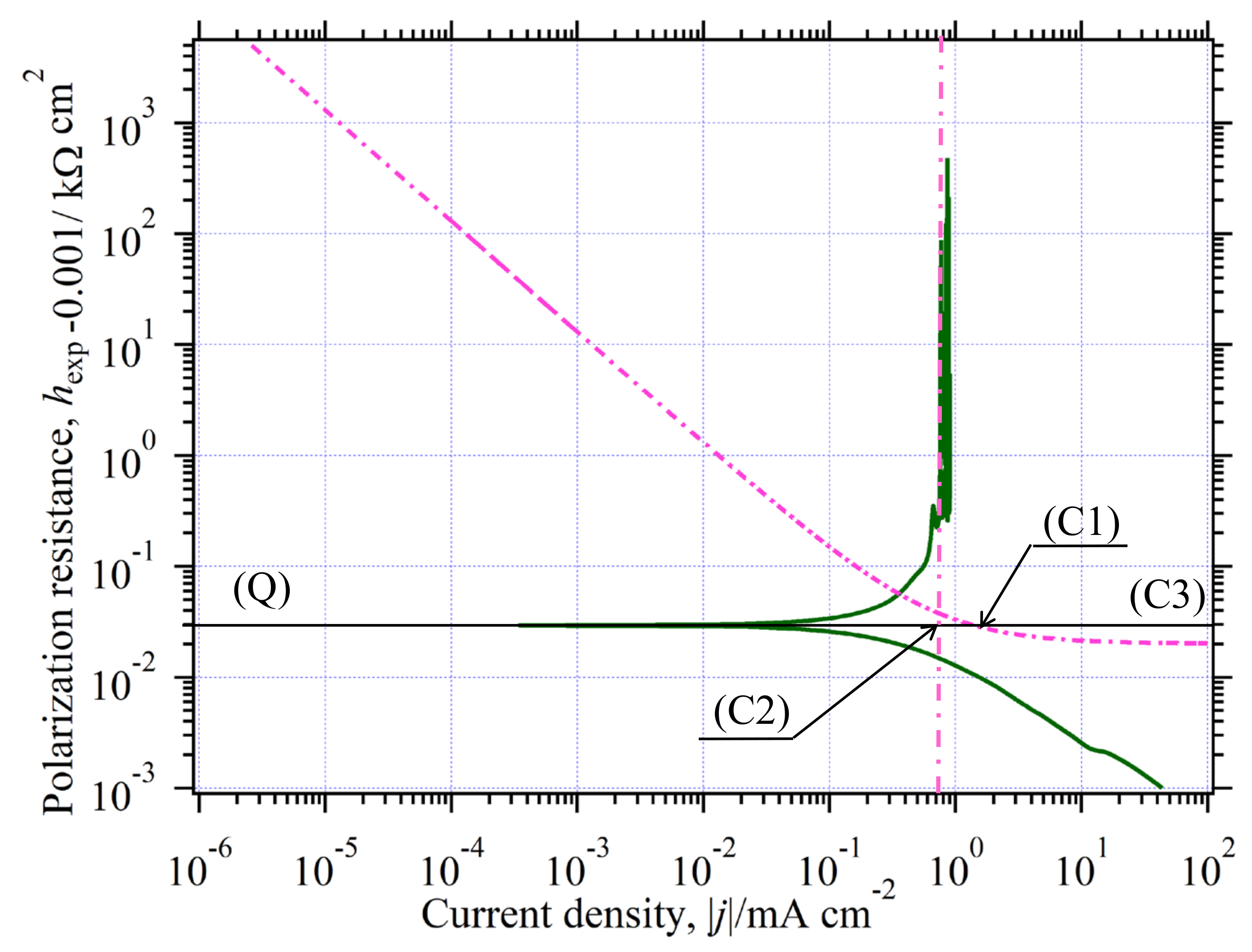
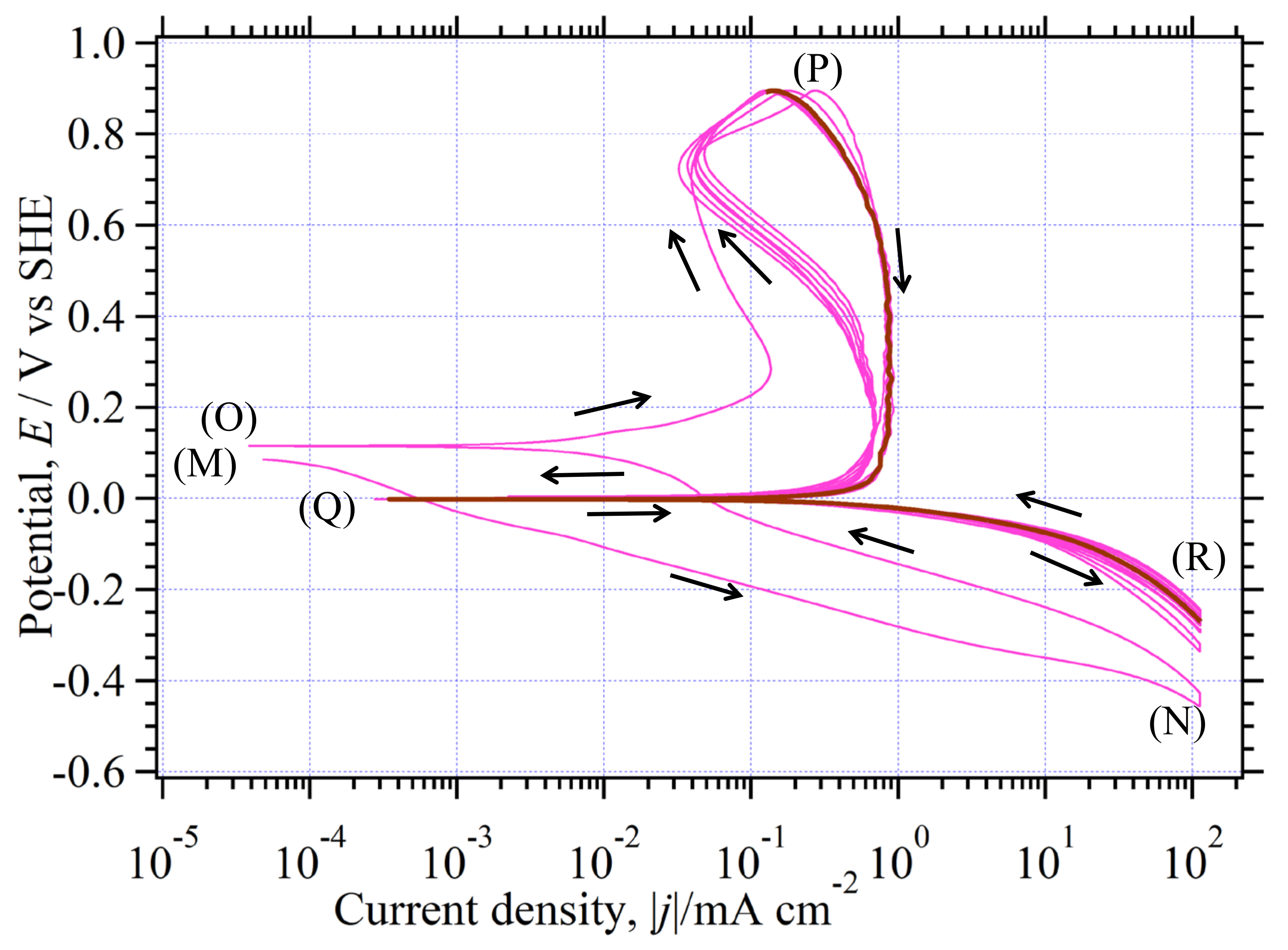
| (Q) in Figure 6 | ||
| (Q) in Figure 7 | ||
| we cannot observe it in Figure 3 | ||
| vertical line having (P) in Figure 7 | ||
| asymptotic horizontal line; (B) in Figure 7 |
| Item | Remarks | |||
|---|---|---|---|---|
| (A): Reversible | (B): Irreversible | (C): Quasi-Reversible | ||
| (j0 ≫ jd) | (j0 ≪ jd) | (j0 ≈ jd) | ||
| 1 | 1 | 1 | ||
| −100 | −100 | −100 | ||
| 0.99 | 0.99 | 0.99 | ||
| 1000 | 0.001 | 1 | ||
| 0.3 | 0.3 | 0.3 | ||
| 0.7 | 0.7 | 0.7 | ||
| 2 | 2 | 2 | ||
| 0.989 | 0.000989 | 0.497 | ||
| 0.013 | 13 | 0.026 | ||
Publisher’s Note: MDPI stays neutral with regard to jurisdictional claims in published maps and institutional affiliations. |
© 2021 by the authors. Licensee MDPI, Basel, Switzerland. This article is an open access article distributed under the terms and conditions of the Creative Commons Attribution (CC BY) license (https://creativecommons.org/licenses/by/4.0/).
Share and Cite
Seri, O.; Furumata, K. Poisoning Effect of CO: How It Changes Hydrogen Electrode Reaction and How to Analyze It Using Differential Polarization Curve. Catalysts 2021, 11, 1322. https://doi.org/10.3390/catal11111322
Seri O, Furumata K. Poisoning Effect of CO: How It Changes Hydrogen Electrode Reaction and How to Analyze It Using Differential Polarization Curve. Catalysts. 2021; 11(11):1322. https://doi.org/10.3390/catal11111322
Chicago/Turabian StyleSeri, Osami, and Kazunao Furumata. 2021. "Poisoning Effect of CO: How It Changes Hydrogen Electrode Reaction and How to Analyze It Using Differential Polarization Curve" Catalysts 11, no. 11: 1322. https://doi.org/10.3390/catal11111322
APA StyleSeri, O., & Furumata, K. (2021). Poisoning Effect of CO: How It Changes Hydrogen Electrode Reaction and How to Analyze It Using Differential Polarization Curve. Catalysts, 11(11), 1322. https://doi.org/10.3390/catal11111322