A Model for Correcting the Pressure Drop between Two Monoliths

Abstract

This paper is concerned with the modeling of the pressure drop through monolith honeycombs. Monolith substrates are promising for the intensification of catalytic processes, especially because of their low back-pressure. There have been several improvements in the modeling of monolith reactors during the last decade, most of them focused on a single substrate configuration, while research in multiple substrates in a single reactor is still sparse. One example is the so-called "minor losses", such as those because of the flow entering and leaving a substrate. Both phenomena interact when two monoliths are placed close in series, and the extra losses produced by them may become relevant when relatively short monoliths are used. In this paper, a spatially resolved computational model of monolith channels arranged in series is used to compute the extra pressure drop because of the flow leaving one substrate and entering the next one downstream. Several Reynolds numbers and spacing lengths for the channels between substrates are investigated. According to the results, for close-coupled monoliths, the inlet and outlet effects produce a negligible pressure drop compared to that in a single monolith configuration. This phenomenon can be accounted for by introducing a correction factor. The magnitude of the correction factor depends on the channel’s Reynolds number, diameter, and spacing length. A model for such a factor is proposed. The model accurately predicts the trend and magnitude of the correction factor.

1. Introduction

Monolith honeycombs are solid pieces with several channels running in parallel that are widely used as catalyst support [1,2,3]. Early monolith reactors in car catalytic converters were typically a single monolith in a carcass [4,5,6]. Now, it is common to find applications with two or more monoliths in series, for example, in automotive exhaust gas after-treatment systems, steam reforming and methanol synthesis [7,8,9,10]. Monoliths present several advantages compared to other catalyst supports. Some of them are low flow resistance, good temperature distribution, and excellent structural integrity. During the last decades, monoliths have been tested in several other industrial applications, such as hydrogenation, peroxide oxidation, and low-temperature Fischer–Tropsch [11,12,13]. 3D-printing and advanced computational models have opened a door for novel substrate configurations, which, in turn, require advanced modeling for systematic optimization [14,15,16,17,18]. One of the main advantages that make monoliths suitable for process intensification is their practically linear relationship between pressure drop and flow rate. In simple terms, the pressure drop through a single honeycomb can be computed as in Equation (1), where $\Delta p_c$ is the pressure drop inside of the substrate and $\Delta p_i$ and $\Delta p_o$ are the head losses because of the flow entering and leaving the substrate respectively [19].

$$\Delta p=\Delta p_i+\Delta p_c+\Delta p_o$$

(1)

For a long monolith, $\Delta p_c$ dominates, so the other terms of Equation (1) can be neglected. On the other hand, although $\Delta p_i$ and $\Delta p_o$ are usually classified as “minor losses”, they depend quadratically on the velocity, so, can become significant at high flow rates in a multiple substrate configuration, especially for monoliths [20,21]. According to previous works, $\Delta p_i$ and $\Delta p_o$ can be modeled as porous jumps [22]. That is, a sudden dissipation of mechanical energy once the flow passes through the inlet and outlet faces of the substrate. Such an approach has a convenient trade-off between simplicity and accuracy but arises questions about the flow behavior when it leaves a substrate and then enters another one placed at a close distance downstream. After leaving the first substrate, the flow progressively develops depending on the channel Re and the operating conditions. Hettel et al. [23] reported a detailed visualization of such a phenomenon. It can be seen that under some circumstances, it may not be reasonable to assume that the head losses because of the flow leaving the substrate take place suddenly, right at the outlet face of the monolith, especially when there is another monolith downstream. If the spacing between the substrates is short, then, the flow pattern from the outcome of the first substrate is modified by the presence of the second substrate, affecting the pressure drop. That topic has not been addressed and is the motivation of this research. This paper has as objective to study and model the pressure drop in the transition between two monoliths arranged in series separated by a short distance. The phenomenon is highly dependent on the interaction between the solid and fluid phases, hence, a spatially resolved geometry is necessary. In that line, a channel scale computational fluid dynamics model was used. The results are presented in terms of pressure and velocity fields. A new model for correcting the pressure drop that considers the length of spacing between substrates is proposed.

2. Computational Model

The domain was composed of two monolith channels placed in series, as shown in Figure 1. The monoliths were considered to have straight square cross-section channels, with 1.1 mm as hydraulic diameter (D) and 0.16 mm as wall thickness ($L_w$). The resulting substrate void fraction ($\varphi$) was approximately 0.76. Such a configuration is fairly similar to those typically found in industrial applications [9,24]. The flow enters and leaves Channel 1, then enters into Channel 2 after traveling a distance $\delta$ through the spacing between the substrates. The length of Channel 1 was 14 mm long, which was sufficient to ensure fully a developed velocity profile at its outlet under all of the conditions tested in this paper. The gap between substrates ($\delta$) varied from 1D to 20D in length, depending on the case analyzed. The open section also had a square transverse shape, with D+$L_w$ as the side. That is, the domain is the fundamental repetitive structure of the two substrates in series. The length of Channel 2 was 5D, which prevented any boundary effect upstream in the zone of interest of this work.

The investigated channel Re were substantially below the critical one, hence, a laminar regime was assumed. There is evidence in the literature that even when the flow approaching a monolith is highly turbulent, it quickly turns to laminar inside of the channels when they operate in a sub-critical condition [25,26].

According to the literature, turbulence may arise also when laminar flow leaves a monolith [27]. Eventual changes in the flow regime in that area were investigated by using Large Eddy Simulation (LES). This is addressed in more detail later in Section 2.2. For the laminar steady model, the mass and momentum conservation equations were [28]:

$$\frac{\partial \left(\rho u_i\right)}{\partial x_i}=0$$

(2)

$$\frac{\partial \left(\rho u_i{u}_j\right)}{\partial x_j}=-\frac{\partial p}{\partial x_i}+\frac{\partial }{\partial x_j}\left[\mu \left(\frac{\partial u_i}{\partial x_j}+\frac{\partial u_j}{\partial x_i}\right)-\frac{2}{3}\frac{\partial u_i}{\partial x_i}{\delta }_{ij}\right]$$

(3)

Notice that all the transport equations in this paper are written in index/suffix notation [29]. The boundary conditions for the laminar case were a prescribed homogeneous velocity for the inlet of Channel 1 and atmospheric pressure at the outlet of Channel 2. The walls of the channels and those representing the frontal and rear faces of the substrates were set as no-slip surfaces. In the open section, the four boundaries (top, bottom, left, and right) were considered free shear surfaces, that is, symmetry planes. The operating fluid was considered atmospheric air at 300 K. The density of the fluid ($\rho$) was computed by using the ideal gas law and the viscosity ($\mu$) according to the kinetic theory of gases [30]. The domain was discretized into a fully orthogonal and homogeneous hexahedral mesh. Since the size of the domain increased together with the length of the gap between substrates, the number of elements of the domain also changed according to the spacing length analyzed, ranging from 1,645,056 to 3,783,168 for the shortest and longest domain, respectively. The size of the elements was kept the same for all the meshes. The problem was implemented in ANSYS Fluent 2021R1 [31], in a 64-core HPC server with two AMD EPYC 7452 CPUs and 256 GB in RAM. A second-order up-wind scheme was used for momentum and the SIMPLE algorithm for the pressure–velocity coupling [32,33]. The stop condition of the simulations was having scaled residuals with a value below 10⁻⁶, together with a stable value for the total pressure drop and maximum velocity magnitude. Those variables are sensitive to the grid quality and relevant for the focus of this paper.

2.1. Grid Quality

The grid independence of the solution was investigated with a channel Re of 200 and spacing between the substrates equivalent to 20D, which should be the most critical condition among those considered in this study. Two grid versions were tested. The first one, referred to as “the original grid”, was that with 3,783,168 elements previously described in Section 2. The second one named “the refined grid”, came from taking the original grid and homogeneously reducing the element’s size, in order to obtain approximately four times more elements, leading to 14,943,513 control volumes. The simulations with the two grids ran until converging. After analyzing the results, the maximum wall $y^{+}$ observed in both cases was below one, the pressure drop and maximum velocity from both grids differed in less than 0.01%, which is fairly negligible, hence, the study continued using the element size of the original mesh.

The quality of the solution was also investigated by calculating the hydraulic entrance length ($L_H$) and Darcy’s friction factor (f) in the fully developed region inside of Channel 1. For $L_H$, the velocity along of the center line of the domain was analyzed. The entrance length was considered to be the distance from the inlet of the channel where the velocity reaches 99% of its asymptotic value, as usual [34]. For the case in Figure 2, which corresponds to a channel Re of 200, the value of $L_H/D·$Re gave 0.0502, which is fairly similar to the classical 0.05 for asquare pipe with a flat inlet velocity profile [35]. According to the Hagen–Poiseuille equation, f can be computed as $2\Delta pD/\Delta x\rho u_c^2$, where $u_c$ is the channel velocity, $\Delta x$ is the length of an arbitrary piece of channel placed in the fully developed region, and $\Delta p$ is the mass-weighted average p across of the channel transverse section [36]. For the case in Figure 2, f in the fully developed region was computed considering a length of $\Delta x$ = D. A value of f = 0.284 was obtained, which leads to fRe = 56.8. Such a value differs in less than 0.2% when compared to the 56.9 reported in the literature for square pipes [37].

2.2. Corroboration of the Flow Regime

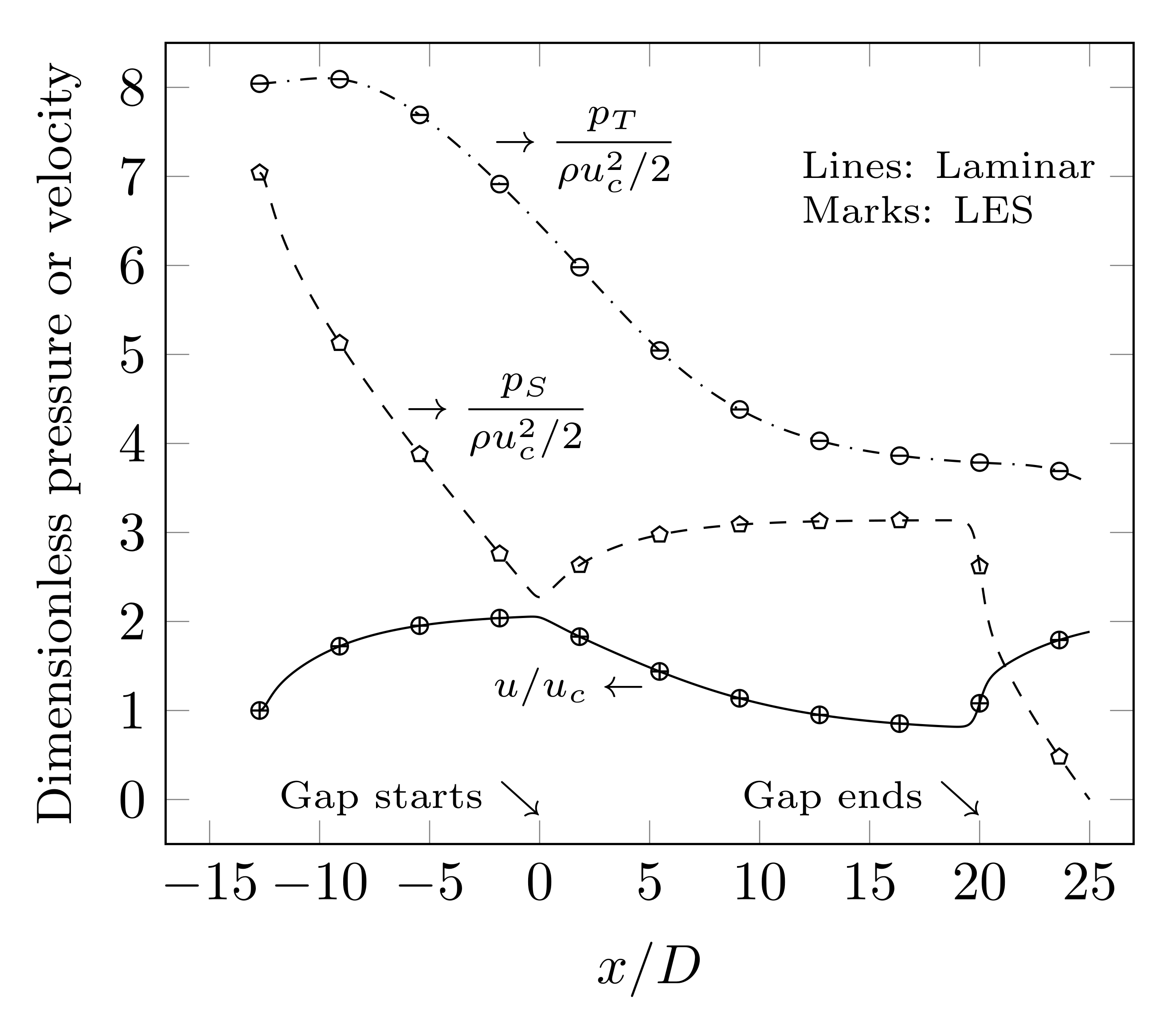
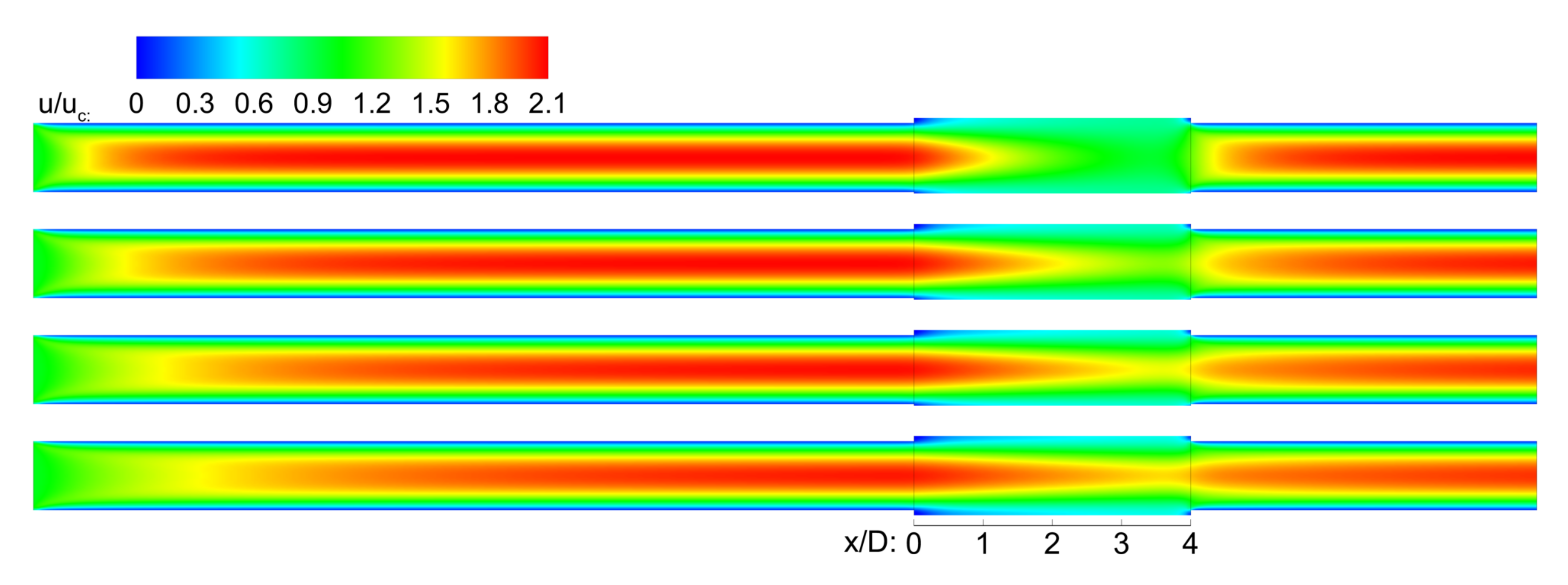
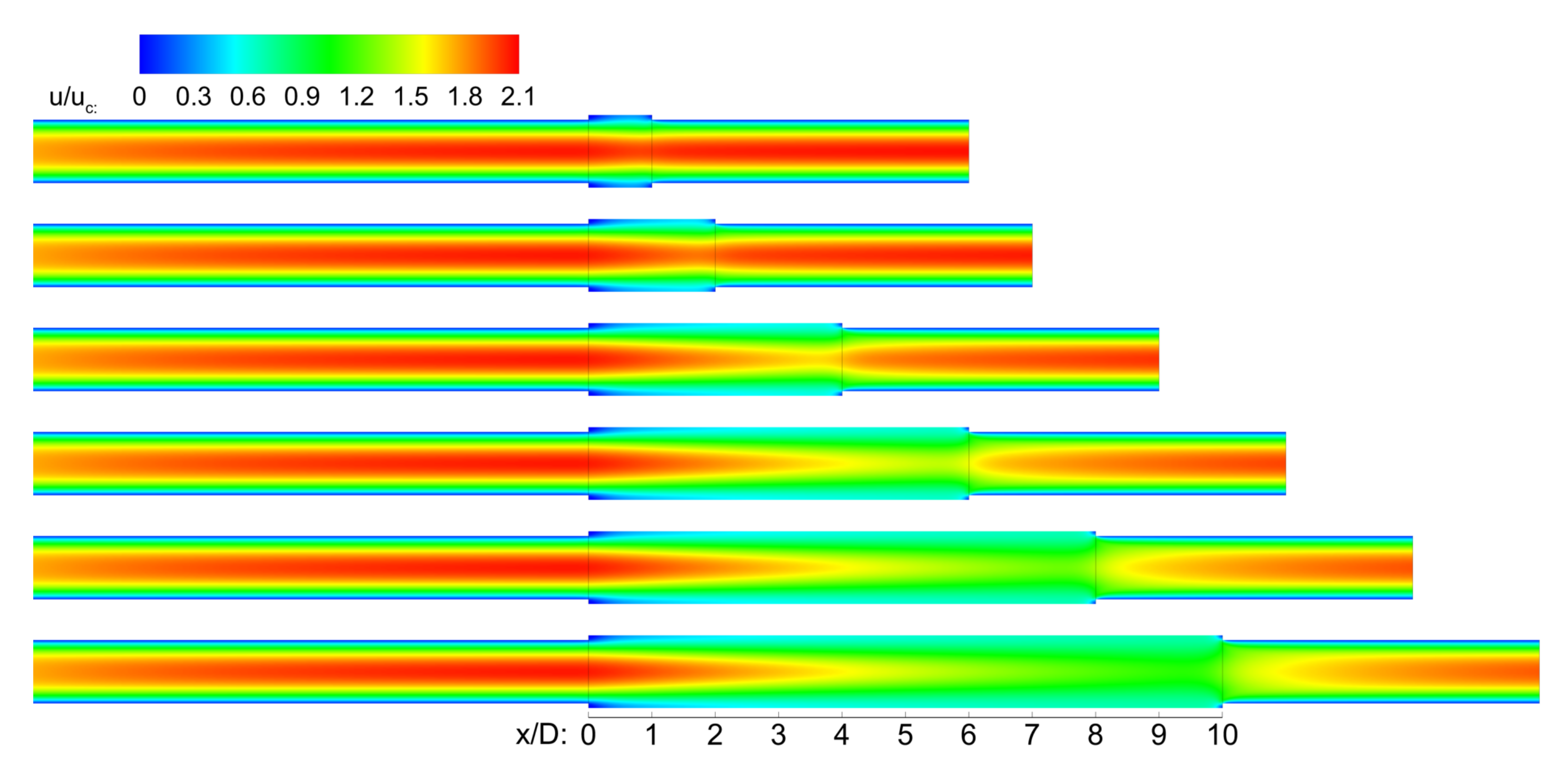
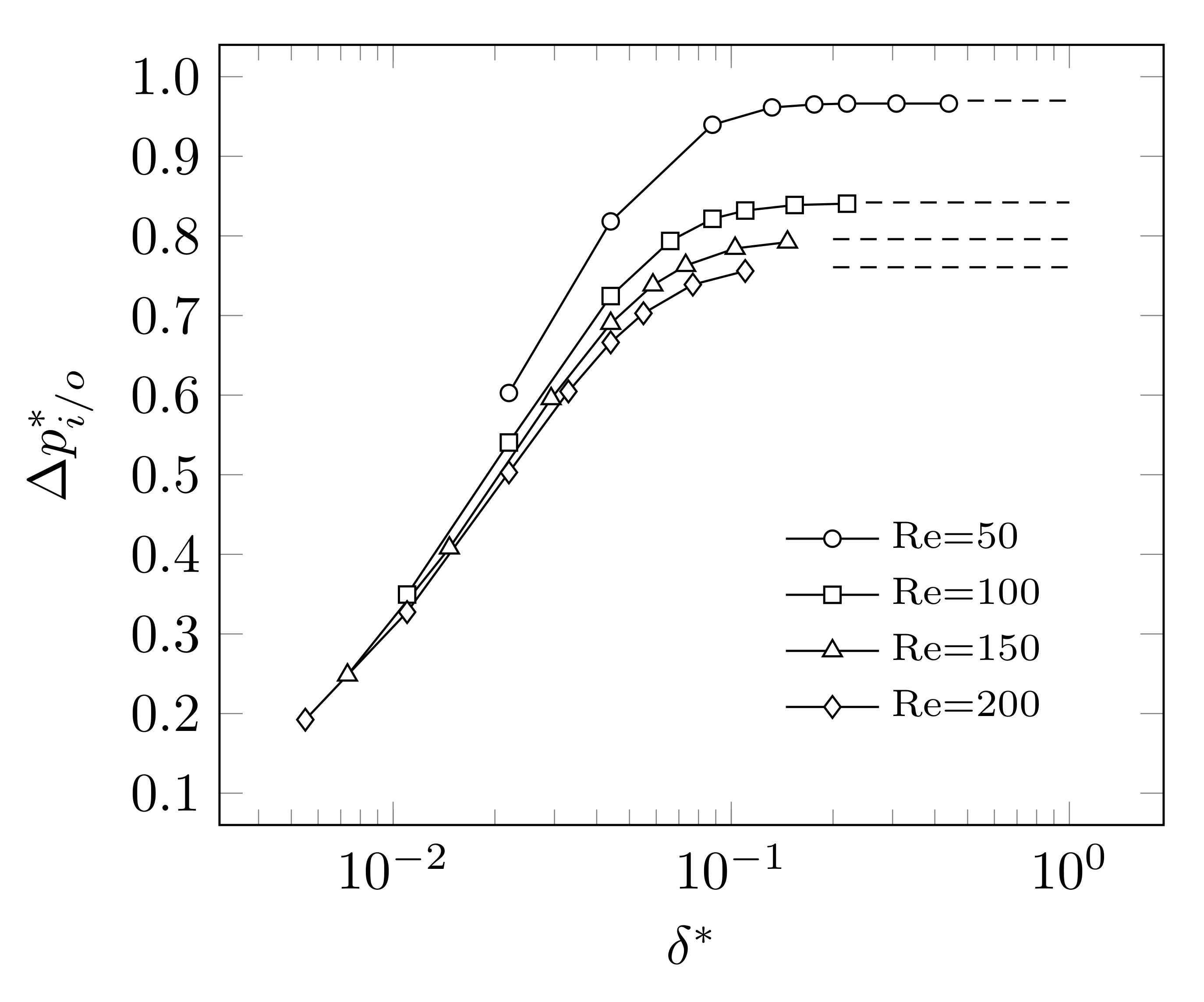
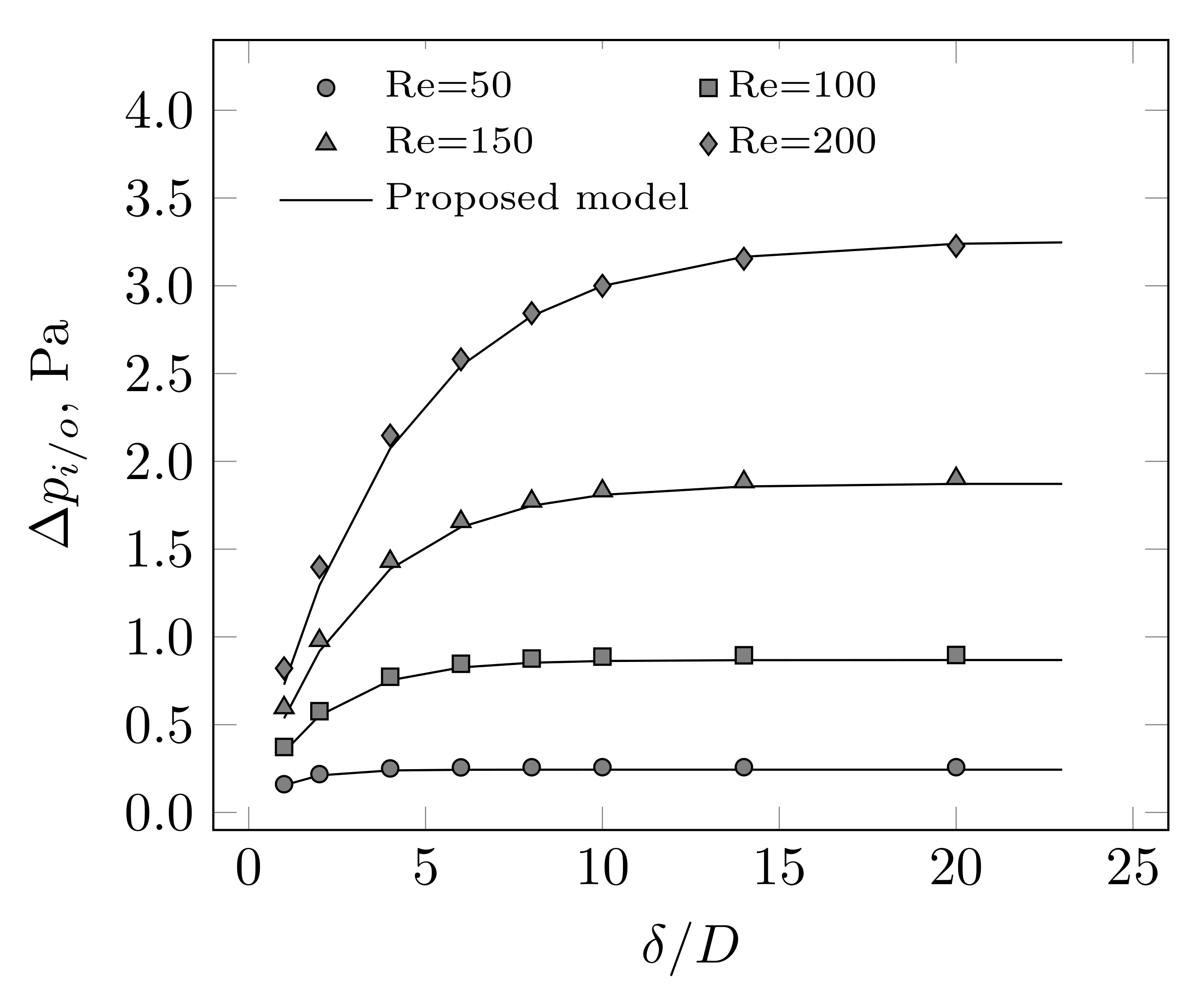
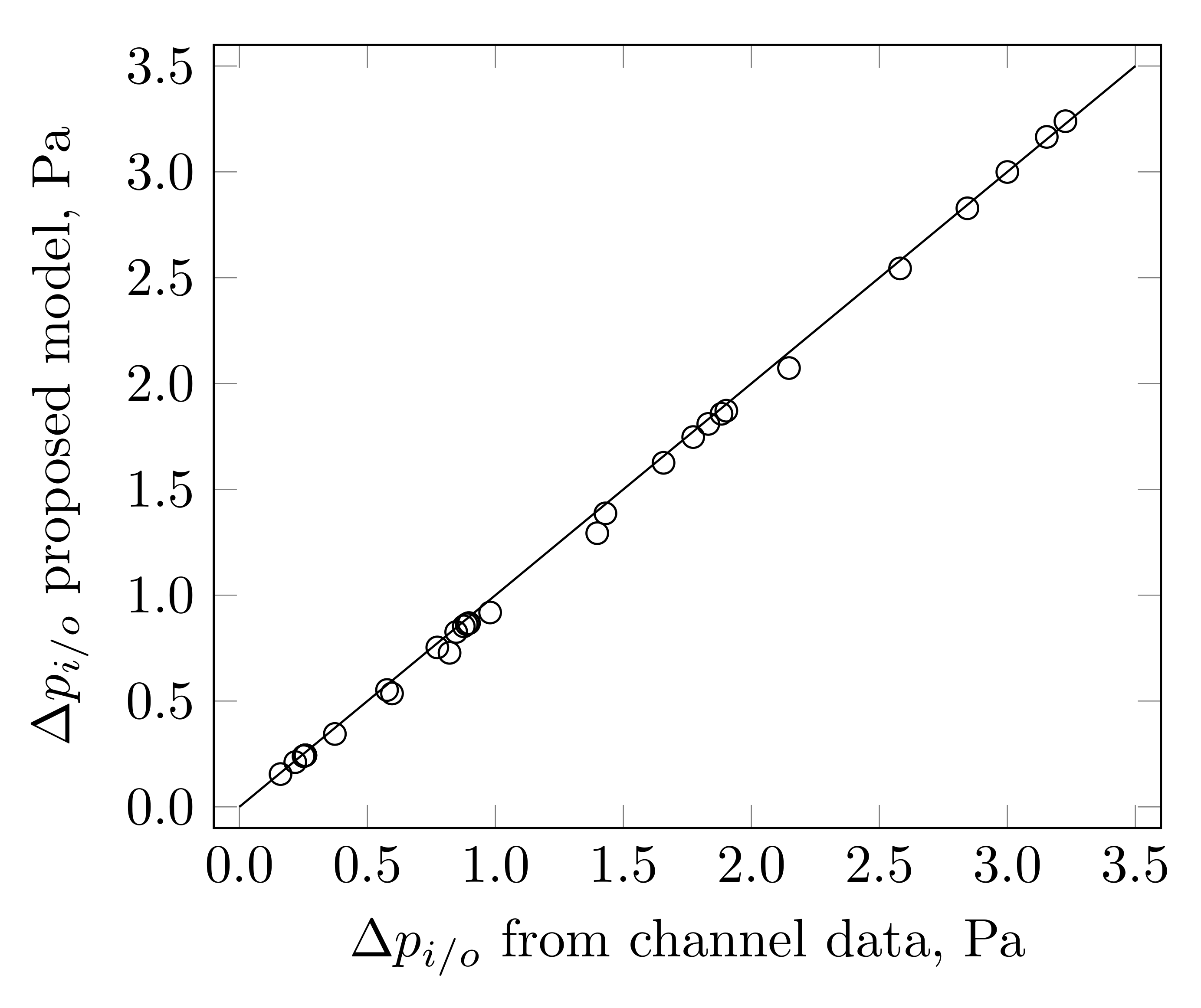
A preliminary analysis was briefly performed in order to corroborate the assumption of steady flow through the entire domain. According to the literature, turbulence may arise as a result of the flow passing around the last part of the substrate walls, or because of the flow behaving as a jet when leaving the channels. Previous works showed that the conditions necessary for those phenomena to take place are not met in this investigation [38]. However, that was investigated in a single substrate configuration and may not be valid for substrates in series. The same scenario as in Section 2.1 was investigated, but using LES instead of a laminar flow model. LES is a high level computational technique, able to predict transitions in the flow regime, from laminar to turbulent and viceversa [39,40]. Turbulent flow is characterized by the presence of a vortex cascade superimposed on the main flow stream. In LES, the large and energetic vortices—or eddies—are resolved directly, while those smaller are modeled in the subgrid domain. In LES, the flow is assumed unsteady and the variables in the resolved and sub-grid scale must be treated separately; hence, the notation in Equations (4)–(8) is exclusive to this section. The mass and momentum balances for LES were the following:

$$\frac{\partial \rho }{\partial t}+\frac{\partial \left(\rho {\overline{u}}_i\right)}{\partial x_j}=0$$

(4)

$$\frac{\partial {\overline{u}}_i}{\partial t}+\overline{u_j}\frac{\partial {\overline{u}}_i}{\partial x_j}=-\frac{1}{\rho }\frac{\partial \overline{p}}{\partial x_i}+\frac{\partial }{\partial x_j}\left(\nu \frac{\partial {\overline{u}}_i}{\partial x_j}+\frac{1}{\rho }\frac{\partial {\tau }_{ij}}{\partial x_j}\right)$$

(5)

The variables with an overline are those from the resolved scale after applying the size filter [39]. The term ${\tau }_{ij}$ was computed as follows:

$${\tau }_{ij}=\frac{2}{3}\rho k_{sgs}{\delta }_{ij}-2C_k{k}^{1/2}{\Delta }_f{\overline{S}}_{ij}$$

(6)

In Equation (6), $k_{sgs}$ is the subgrid-scale kinetic energy, which was modeled with the DKE model [41]. In this subgrid model, $k_{sgs}$ is treated as a conservative quantity, with the following transport equation:

$$\frac{\partial \left(\rho k_{sgs}\right)}{\partial t}+\frac{\partial \left(\rho {\overline{u}}_j{k}_{sgs}\right)}{\partial x_j}=-{\tau }_{ij}\frac{\partial {\overline{u}}_i}{\partial x_j}-C_{\epsilon }\rho \frac{k_{sgs}^{3/2}}{{\Delta }_f}+\frac{\partial }{\partial x_j}\left(\frac{{\mu }_{sgs}}{{\sigma }_k}\frac{\partial k_{sgs}}{\partial x_i}\right)$$

(7)

where

$${\mu }_{sgs}=k\rho k_{sgs}^{1/2}{\Delta }_f$$

(8)

Interested readers are referred to the following references for additional details about the parameters and sub-functions of the DKE model [28,41]. As mentioned, for LES, the domain with a gap between channels 20D long and a channel Re of 200 was considered. The grid was the one with 3,783,168 control volumes previously described in Section 2.1. In the inlet, $k_{sgs}$ was set as zero. In contrast with the laminar case, the four boundaries in the open section were set as periodic, mirroring top-bottom and left-right. That makes the model more sensitive to eventual turbulence triggering in that region [38]. The time step size was manipulated to obtain a CFL number below one, which led to values of the order of 10⁻⁵ s. The unsteady term was discretized with a bounded second-order accuracy implicit scheme and momentum by bounded central differencing [28]. The stop condition for every time step was having scaled residuals smaller than 10⁻⁴. The simulation was initialized by taking as a reference the inlet values, then ran. The simulation was planned to run for a time window sufficiently long for the flow to pass through the whole domain twice, then starting to collect data to monitor the average pressure and velocity fields. However, after approximately four thousand time steps (≈41 ms), the solution converged to a steady one. That is, the maximum and minimum value of the scaled residuals progressively decreased with every iteration, until observing no change between successive time steps. The solution obtained was practically the same as that when using the laminar flow model. Marks with the data from LES were included in Figure 2. The velocity and pressure fields, so the friction factor and pressure drop, from LES were fairly similar to those from the laminar case. After stopping the simulation, it was observed that $k_{sgs}$ was zero through all the domains. That corroborates that turbulence does not arise in the conditions of this study, so, the rest of the paper continued with a laminar flow model.

3. Results

This section summarizes the results obtained. Channel Re ranging from 50 to 200 and channels spacing between 1D and 20D were considered. The full list of the computational runs analyzed is shown in

Table 1. List of the 32 computational runs.

N	Re	$\mathit{\delta }$/D	N	Re	$\mathit{\delta }$/D	N	Re	$\mathit{\delta }$/D	N	Re	$\mathit{\delta }$/D
1	50	1	9	50	4	17	50	8	25	50	14
2	100	1	10	100	4	18	100	8	26	100	14
3	150	1	11	150	4	19	150	8	27	150	14
4	200	1	12	200	4	20	200	8	28	200	14
5	50	1	13	50	6	21	50	10	29	50	20
6	100	2	14	100	6	22	100	10	30	100	20
7	150	2	15	150	6	23	150	10	31	150	20
8	200	2	16	200	6	24	200	10	32	200	20

.

First, a qualitative analysis was performed. Figure 3 shows the velocity field along the center plane of the domain for an increasing Re, at a constant spacing between channels. Clearly, the flow profile inside of square channels is not axially symmetrical, however, the center planes contain the maximum velocity and are useful to provide an insight of the flow development [42,43]. It can be seen from the figure that in the case of Re = 50, a distance of x/D = 4 is sufficient for the flow to achieve a reasonably flat velocity profile in the open section. The scaled average velocity in that area should be $u/u_c$ = $\varphi$ = 0.76, which lies in the green area of the color scale, corroborating the expected asymptotic velocity. This is also consistent with the scaled velocity in Figure 2. Under these circumstances, it is reasonable to assume that the formulas to estimate $\Delta p_i$ and $\Delta p_o$ in a single monolith configuration are still valid because the flow in both channels do not interact. For the other cases, a convex velocity profile remained after exiting the channel for a distance that increased together with Re. Here, interactions between the flow leaving Channel 1 and entering Channel 2 do occur. This was especially noticeable in the case with Re = 200, where the viscous core of Channel 1 is fully connected to that of Channel 2.

Figure 4 shows the velocity field at a constant Re for several spacing lengths. The interaction of the flow in both channels is more evident in the case with the shortest spacing, where the flow passes from one channel to the other remaining almost unaltered along of the gap. In such a case, calculating the pressure drop in the transition between the substrates ($\Delta p_{i/o}$) as the summation of $\Delta p_o$ of Channel 1 and $\Delta p_i$ of Channel 2 clearly results in an overestimation. That is explained by the fact that there is not sufficient space for the arrangement of the flow lamina after leaving the first substrate, so, the collision of the flow with the frontal face of the second substrate is partially diminished. This attenuating effect on $\Delta p_{i/o}$ seems to progressively decrease as the spacing between substrates increases (or Re decreases), until the point where it becomes negligible, and $\Delta p_{i/o}$ equals $\Delta p_i$+$\Delta p_o$.

Both $\Delta p_i$ and $\Delta p_o$ for a single monolith configuration can be estimated by using Equations (9) and (10). In the equations, $f_1$ and $f_2$ are polynomials that depend on the channel cross-section shape and substrate void fraction. All were taken from [19].

$$\Delta p_i=f_1{|}_i\mu u_c+f_2{|}_i\frac{1}{2}\rho u_c^2$$

(9)

$$\Delta p_o=f_2{|}_o\frac{1}{2}\rho u_c^2$$

(10)

The value of $\Delta p_{i/o}$ can be also quantified from the CFD results by using in Equation (11), where $P_1$ is a plane at the rear face of Channel 1, $P_2$ that at the frontal face of Channel 2, and A is the transverse area of the respective cross-sections (see Figure 1). In the equation, $p_T$ is the total pressure (static plus dynamic) and is weighted by the mass flow across of the respective transverse section, which is necessary to keep consistency with the momentum balance and to compute the correct head losses when the velocity profile or flow area are non-constant.

$$\Delta p_{i/o}=\frac{{\int }_A\rho u{p}_{T}dA}{{\int }_A\rho udA}{|}_{P_1}-\frac{{\int }_A\rho u{p}_{T}dA}{{\int }_A\rho udA}{|}_{P_2}$$

(11)

Figure 5 shows $\Delta p_{i/o}$ for several channel Re and spacing lengths. Consistently with the observed velocity fields, the pressure drop between substrates increases together with Re and gap length. The curves in the figure show a decreasing sensitivity as the gap length increases. It is also corroborated from the CFD data that the asymptotic value of every curve corresponds to $\Delta p_i$+$\Delta p_o$ for a given Re. This happens when the spacing between substrates is sufficient to achieve a developed profile in the open section, allowing us to treat the flow leaving the first substrate and entering into the second one essentially as two fully decoupled phenomena.

The data in Figure 5 was non-dimensionalized according to Equation (12) and plot in Figure 6. The x-axis was put in log-scale to emphasize the non-asymptotic part of the curve. It should be noticed that $x^{*}$ is defined identically as the classical $x^{+}$, however, for consistency in the notation, a star was used as superscript in all of the dimensionless variables in this paper. It is also important to mention that the gap between channels was computed as $\delta$ = $x-x_0$, where $x_0$ is the axial position of the exit of Channel 1. For simplicity, $x_0$ = 0 was used as reference, leading to an equivalent definition for $x^{*}$ and ${\delta }^{*}$, but the conceptual difference between the two variables must be distinguished.

$$x^{*}=\frac{x}{D·\mathrm{Re}};\Delta p_i^{*}=\frac{\Delta p_i}{\frac{1}{2}\rho u_c^2};\Delta p_o^{*}=\frac{\Delta p_o}{\frac{1}{2}\rho u_c^2};\Delta p_{i/o}^{*}=\frac{\Delta p_{i/o}}{\frac{1}{2}\rho u_c^2}{\delta }^{*}=\frac{x}{D·\mathrm{Re}}$$

(12)

It seems that all of the curves in Figure 6 can be projected towards the same source point. Regarding the asymptotic value, it corresponds to the respective ($\Delta p_i^{*}$+$\Delta p_o^{*}$) for each of their respective Re, similar to their counterpart data with dimensions (see Figure 5). It can be noticed from the figure that all of the curves reach the 0.99 of their asymptotic value at approximately the same value of ${\delta }^{*}$. Such a behavior is typical of a first-order linear differential system as that in Equation (13).

$${\tau }_c{\zeta }^{\prime }+\zeta =k_c\eta$$

(13)

where ${\tau }_c$ and $k_c$ are constants, $\zeta$ is $\Delta p_{i/o}^{*}$ and $\eta$ is ($\Delta p_i^{*}$+$\Delta p_o^{*}$). That ordinary differential equation can be easily solved by using Laplace transform or an exponent integrating factor, leading to an algebraic solution as that in Equation (14) [44,45].

$$\Delta p_{i/o}^{*}=k_c[1-e^{{\tau }_c{\delta }^{*}}]\left(\Delta p_i^{*}+\Delta p_o^{*}\right)$$

(14)

The values for $k_c$ and ${\tau }_c$ can be obtained by a least square fit between Equation (14) and the data in Figure 6 [46]. The fitting gives the following values with their 95% confidence intervals $k_c$ = 1.03 ± 0.04 and ${\tau }_c$ = 45.92 ± 0.15. Analyzing the equation, $k_c[1-e^{-{\tau }_c{\delta }^{*}}]$ works as a sort of correction factor ($f_{\delta }$), which asymptotic value is precisely $k_c$. Taking into account its confidence interval, $k_c$ is reasonably close to the unit, so, if ${\delta }^{*}\to \infty$, then $\Delta p_{i/o}^{*}\to (\Delta p_i^{*}$+$\Delta p_i^{*}$), as expected.

It is interesting to find out from what spacing length a correction to the pressure drop is not needed. Let us define that a 1% error in the dimensionless pressure drop is acceptable. Dropping $k_c$, such an accuracy is achieved approximately when $[1-e^{-{\tau }_c{\delta }^{*}}]$ = 0.99. Solving for ${\delta }^{*}$, it gives approximately ${\delta }^{*}$ = 0.1 (notice that this value can be read from Figure 6 also). That is, if the spacing between substrates meets $\delta >0.1D·$Re, then, no correction factor is needed and $\Delta p_{i/o}^{*}$ is reasonably approximated by ($\Delta p_i^{*}$ + $\Delta p_i^{*}$). Notice that $f_{\delta }$ is dimensionless, hence, it can be applied to both $\Delta p$ or its non-dimensionalized version $\Delta p^{*}$, as follows:

$$f_{\delta }={\displaystyle \frac{\Delta p_{i/o}}{\Delta p_i+\Delta p_o}}={\displaystyle \frac{\Delta p_{i/o}^{*}}{\Delta p_i^{*}+\Delta p_o^{*}}}=1-exp(-{\tau }_c\delta /D·\mathrm{Re})$$

(15)

Figure 7 shows the data from CFD together with the prediction from the proposed model in Equation (14). In the plot, $k_c$ was assumed to be one. The agreement remained fairly reasonable for the curves of all of the cases analyzed. Finally, a correlation plot is shown in Figure 8. It can be seen that all of the predicted values are consistent both in magnitude and trend with the CFD. All of them are placed in the 45° line region also.

Finally,

Table 2. Range of application of the proposed model.

Gap Length ($\mathit{\delta }$)	Correction (${\mathit{f}}_{\mathit{\delta }}$)	$\Delta {\mathit{p}}_{\mathit{i}/\mathit{o}}$
$\delta \ge 0.1D·$Re	1	$\Delta p_i$ + $\Delta p_o$
$0.1D·\mathrm{Re}>\delta >0.001D·\mathrm{Re}$	$1-exp(-45.92\delta /D·\mathrm{Re})$	$f_{\delta }$($\Delta p_i$ + $\Delta p_o$)
$0.01D·$Re$\ge \delta$	0	0

summarizes the criterion to consider that the spacing length is short, intermediate, or long, together with the correction factor proposed for every case.

The model was calibrated for square straight channels, but, in industrial applications, there are substrates with triangular, circular, hexagonal, and other channel shapes also [47,48,49,50]. For those case, the values for $k_c$ and ${\tau }_c$ may differ from those presented in Table 2. When comparing other relevant variables for different channel shapes, such as friction factor and Nusselt number, it can be noted that their values typically vary by the same order of magnitude [35,37]. Based on that, it can be expected that this model still may provide an approximation for correction factors for other channel geometries. However, if high accuracy is required, then the model must be properly calibrated for each specific channel shape.

4. Conclusions

The pressure drop between two monoliths with identical cell densities was investigated by using a computational model. In substrates in an in-series configuration, if the spacing between substrates is sufficiently long, then the flow leaving one substrate and entering into the next one can be treated as two separated phenomena. If the substrates are close-coupled, then a correction factor is needed to compute the correct pressure drop in the gap. The correction factor increases together with the gap length and decreases with the channel Re. A model that describes accurately the trend and magnitude of such a factor is proposed. The correction factor ranges between zero and one. If the gap length is greater or equal than 0.1D·Re, then no correction is needed. On the other hand, if that length is smaller or equal to 0.001D·Re, then the pressure drop because of the flow leaving one substrate and entering the next one can be neglected. For the cases in between, if the correction is not considered, then the aforementioned head losses are overestimated.

The generation of turbulence because of the flow leaving the monolith was also analyzed by using LES. According to the results, placing the two monoliths in series and separated by a long distance did not affect the flow regime in the open area between them. This was analyzed for substrates inline and may not apply in other circumstances.

The results and models presented in this paper are consistent with the expected from a theoretical standpoint, however, further experimental validation is recommended. The model may provide an estimation for the value of the correction factor for other channel shapes, but that still needs to be corroborated.

References

1. Williams, J.L. Monolith structures, materials, properties and uses. Catal. Today 2001, 69, 3–9. [Google Scholar] [CrossRef]
2. Hayes, R.E.; Cornejo, I. Multi-scale modelling of monolith reactors: A 30-year perspective from 1990 to 2020. Can. J. Chem. Eng. 2021. [Google Scholar] [CrossRef]
3. Lock, J.; Clasén, K.; Sjoblom, J.; McKelvey, T. A Control-Oriented Spatially Resolved Thermal Model of the Three-Way-Catalyst; SAE International: Warrendale, PA, USA, 2021; Available online: https://www.sae.org/publications/technical-papers/content/2021-01-0597 (accessed on 1 August 2021).
4. Clarkson, R.J. A Theoretical and Experimental Study of Automotive Catalytic Converters. Ph.D. Thesis, Coventry University, Coventry, UK, 1997. [Google Scholar]
5. Della Torre, A.; Montenegro, G.; Onorati, A.; Cerri, T.; Tronconi, E.; Nova, I. Numerical Optimization of a SCR System Based on the Injection of Pure Gaseous Ammonia for the NOx Reduction in Light-Duty Diesel Engines. In Proceedings of the SAE 2020 World Congress Experience, Detroit, MI, USA, 21–23 April 2020; pp. 1–11. [Google Scholar]
6. Benjamin, S.F.; Clarkson, R.; Haimad, N.A.; Girgis, N. An experimental and predictive study of the flow field in axisymmetric automotive exhaust catalyst systems. SAE Trans. 1996, 105, 1008–1019. [Google Scholar]
7. Tahay, P.; Khani, Y.; Jabari, M.; Bahadoran, F.; Safari, N. Highly porous monolith/TiO2 supported Cu, Cu-Ni, Ru, and Pt catalysts in methanol steam reforming process for H2 generation. Appl. Catal. A Gen. 2018, 554, 44–53. [Google Scholar] [CrossRef]
8. Chatterjee, D.; Burkhardt, T.; Rappe, T.; Güthenke, A.; Weibel, M. Numerical simulation of DOC+ DPF+ SCR systems: DOC influence on SCR performance. SAE Int. J. Fuels Lubr. 2009, 1, 440–451. [Google Scholar] [CrossRef]
9. Arab, S.; Commenge, J.M.; Portha, J.F.; Falk, L. Methanol synthesis from CO2 and H2 in multi-tubular fixed-bed reactor and multi-tubular reactor filled with monoliths. Chem. Eng. Res. Des. 2014, 92, 2598–2608. [Google Scholar] [CrossRef]
10. Jang, J.; Lee, J.; Choi, Y.; Park, S. Reduction of particle emissions from gasoline vehicles with direct fuel injection systems using a gasoline particulate filter. Sci. Total Environ. 2018, 644, 1418–1428. [Google Scholar] [CrossRef]
11. Martínez, F.L.D.; Julcour, C.; Billet, A.M.; Larachi, F. Modelling and simulations of a monolith reactor for three-phase hydrogenation reactions—Rules and recommendations for mass transfer analysis. Catal. Today 2016, 273, 121–130. [Google Scholar] [CrossRef] [Green Version]
12. Quintanilla, A.; Casas, J.; Miranzo, P.; Osendi, M.I.; Belmonte, M. 3D-Printed Fe-doped silicon carbide monolithic catalysts for wet peroxide oxidation processes. Appl. Catal. B Environ. 2018, 235, 246–255. [Google Scholar] [CrossRef]
13. Ibáñez, M.; Sanz, O.; Egaña, A.; Reyero, I.; Bimbela, F.; Gandía, L.M.; Montes, M. Performance comparison between washcoated and packed-bed monolithic reactors for the low-temperature Fischer-Tropsch synthesis. Chem. Eng. J. 2021, 425, 130424. [Google Scholar] [CrossRef]
14. Busse, C.; Freund, H.; Schwieger, W. Intensification of heat transfer in catalytic reactors by additively manufactured periodic open cellular structures (POCS). Chem. Eng. Process.-Process. Intensif. 2018, 124, 199–214. [Google Scholar] [CrossRef]
15. Negri, M.; Wilhelm, M.; Hendrich, C.; Wingborg, N.; Gediminas, L.; Adelöw, L.; Maleix, C.; Chabernaud, P.; Brahmi, R.; Beauchet, R.; et al. New technologies for ammonium dinitramide based monopropellant thrusters–The project RHEFORM. Acta Astronaut. 2018, 143, 105–117. [Google Scholar] [CrossRef]
16. Souliotis, T.; Koltsakis, G.; Samaras, Z. Catalyst Modeling Challenges for Electrified Powertrains. Catalysts 2021, 11, 539. [Google Scholar] [CrossRef]
17. Cornejo, I.; Hayes, R.E. A Review of the Critical Aspects in the Multi-Scale Modelling of Structured Catalytic Reactors. Catalysts 2021, 11, 89. [Google Scholar] [CrossRef]
18. Walander, M.; Nygren, A.; Sjöblom, J.; Johansson, E.; Creaser, D.; Edvardsson, J.; Tamm, S.; Lundberg, B. Use of 3D-printed mixers in laboratory reactor design for modelling of heterogeneous catalytic converters. Chem. Eng. Process.-Process. Intensif. 2021, 164, 108325. [Google Scholar] [CrossRef]
19. Cornejo, I.; Nikrityuk, P.; Hayes, R.E. The influence of channel geometry on the pressure drop in automotive catalytic converters: Model development and validation. Chem. Eng. Sci. 2020, 212, 115317. [Google Scholar] [CrossRef]
20. Carter, R.N.; Menacherry, P.; Pfefferle, W.C.; Muench, G.; Roychoudhury, S. Laboratory Evaluation of Ultra-Short Metal Monolith Catalyst; Technical Report; SAE Technical Paper; SAE International: Warrendale, PA, USA, 1998. [Google Scholar]
21. Quadri, S. The Effect of Oblique Entry Flow in Automotive Catalytic Converters. Ph.D. Thesis, Coventry University, Coventry, UK, 2008. [Google Scholar]
22. Cornejo, I.; Nikrityuk, P.; Hayes, R.E. Pressure correction for automotive catalytic converters: A multi-zone permeability approach. Chem. Eng. Res. Des. 2019, 147, 232–243. [Google Scholar] [CrossRef]
23. Hettel, M.; Daymo, E.; Schmidt, T.; Deutschmann, O. CFD-Modeling of fluid domains with embedded monoliths with emphasis on automotive converters. Chem. Eng. Process.-Process. Intensif. 2020, 147, 107728. [Google Scholar] [CrossRef]
24. Hayes, R.E.; Fadic, A.; Mmbaga, J.; Najafi, A. CFD modelling of the automotive catalytic converter. Catal. Today 2012, 188, 94–105. [Google Scholar] [CrossRef]
25. Cornejo, I.; Nikrityuk, P.; Lange, C.; Hayes, R.E. Influence of upstream turbulence on the pressure drop inside a monolith. Chem. Eng. Process.-Process. Intensif. 2020, 147, 107735. [Google Scholar] [CrossRef]
26. Cornejo, I.; Hayes, R.E.; Nikrityuk, P. A new approach for the modeling of turbulent flows in automotive catalytic converters. Chem. Eng. Res. Des. 2018, 140, 308–319. [Google Scholar] [CrossRef]
27. Cornejo, I.; Nikrityuk, P.; Hayes, R.E. Effect of substrate geometry and flow condition on the turbulence generation after a monolith. Can. J. Chem. Eng. 2020, 98, 947–956. [Google Scholar] [CrossRef]
28. ANSYS Fluent Theory Guide Release 2021R1; ANSYS Inc.: Canonsburg, PA, USA, 2021.
29. Tyldesley, J.R. An Introduction to Tensor Analysis for Engineers and Applied Scientists; Longman Publishing Group: Upper Saddle River, NJ, USA, 1975. [Google Scholar]
30. Kauzmann, W. Kinetic Theory of Gases; Courier Corporation: New York, NY, USA, 2012. [Google Scholar]
31. ANSYS Fluent Software Package v2021R1; ANSYS Inc.: Canonsburg, PA, USA, 2021.
32. Patankar, S. Numerical Heat Transfer and Fluid Flow; CRC Press: Boca Raton, FL, USA, 1980. [Google Scholar]
33. Malalasekera, W.; Versteeg, H. An Introduction to Computational Fluid Dynamics: The Finite Volume Method; PEARSON Prentice Hall: Upper Saddle River, NJ, USA, 2007. [Google Scholar]
34. Shah, R. A correlation for laminar hydrodynamic entry length solutions for circular and noncircular ducts. J. Fluids Eng. 1978, 100, 177–179. [Google Scholar] [CrossRef]
35. Bergman, T.L.; Incropera, F.P.; DeWitt, D.P.; Lavine, A.S. Fundamentals of Heat and Mass Transfer; John Wiley & Sons: New York, NY, USA, 2011. [Google Scholar]
36. Durst, F. Fluid Mechanics: An Introduction to the Theory of Fluid Flows; Springer Science & Business Media: Berlin/Heidelberg, Germany, 2008. [Google Scholar]
37. White, F.M. Fluid Mechanics; McGraw-Hill: New York, NY, USA, 2009. [Google Scholar]
38. Cornejo, I.; Nikrityuk, P.; Hayes, R.E. Turbulence generation after a monolith in automotive catalytic converters. Chem. Eng. Sci. 2018, 187, 107–116. [Google Scholar] [CrossRef]
39. Menon, S.; Yeung, P.K.; Kim, W.W. Effect of subgrid models on the computed interscale energy transfer in isotropic turbulence. Comput. Fluids 1996, 25, 165–180. [Google Scholar] [CrossRef]
40. Menon, S.; Kim, W.W. High Reynolds number flow simulations using the localized dynamic subgrid-scale model. In Proceedings of the 34th Aerospace Sciences Meeting and Exhibit, Reno, NV, USA, 15–18 January 1996; p. 425. [Google Scholar]
41. Kim, W.W.; Menon, S.; Kim, W.W.; Menon, S. Application of the localized dynamic subgrid-scale model to turbulent wall-bounded flows. In Proceedings of the 35th Aerospace Sciences Meeting and Exhibit, Reno, NV, USA, 6–10 January 1997; p. 210. [Google Scholar]
42. Afzal, N.; Seena, A.; Bushra, A. Power law velocity profile in fully developed turbulent pipe and channel flows. J. Hydraul. Eng. 2007, 133, 1080–1086. [Google Scholar] [CrossRef]
43. Peszynski, K.; Tesař, V. Algebraic model of turbulent flow in ducts of rectangular cross-section with rounded corners. Flow Meas. Instrum. 2020, 75, 101790. [Google Scholar] [CrossRef]
44. Blanchard, P.; Devaney, R.; Hall, G. Differential Equations; Richard Stratton: Boston, MA, USA, 2011. [Google Scholar]
45. Kreyszig, E. Advanced Engineering Mathematics; John Wiley & Sons: New York, NY, USA, 2011. [Google Scholar]
46. Montgomery, D.C. Design and Analysis of Experiments; John Wiley & Sons: New York, NY, USA, 2017. [Google Scholar]
47. Iwaniszyn, M.; Jodłowski, P.J.; Sindera, K.; Gancarczyk, A.; Korpyś, M.; Jędrzejczyk, R.J.; Kołodziej, A. Entrance effects on forced convective heat transfer in laminar flow through short hexagonal channels: Experimental and CFD study. Chem. Eng. J. 2021, 405, 126635. [Google Scholar] [CrossRef]
48. Groppi, G.; Tronconi, E. Theoretical analysis of mass and heat transfer in monolith catalysts with triangular channels. Chem. Eng. Sci. 1997, 52, 3521–3526. [Google Scholar] [CrossRef]
49. Watling, T.C. Flow and Forced Convection Heat and Mass Transfer Characteristics of Developed Laminar Flow in Square Channels with Rounded Corners: A Model for Flow in Washcoated Monolith Channels. Ind. Eng. Chem. Res. 2020, 59, 19770–19780. [Google Scholar] [CrossRef]
50. Watling, T.C.; Van Lishout, Y.; Rees, I.D. Backpressure Prediction for Flow-Through Monoliths and Wall-Flow Filters Using 1-Dimensional Models: Entrance Effect Pressure Change, Developing Flow and Validation Using Length-Varying Techniques. Emiss. Control. Sci. Technol. 2021, 1–18. [Google Scholar] [CrossRef]
Figure 1. Schematic of the domain. P 1 and P 2 are transverse planes at the outlet of Channel 1 and inlet of Channel 2, respectively.
Catalysts 11 01314 g001
Figure 2. Comparison of the results from the laminar and LES models. For LES, the values correspond to the final steady state solution. Channel Re was 200. p T is total pressure, p S is static pressure, and u is velocity magnitude. For this figure, p T , p S , and u were taken from the center line along of the domain; hence, are local values but non-dimensionalized by using the channel velocity.
Catalysts 11 01314 g002
Figure 3. Effect of increasing Re at a constant spacing between substrates. Channel Re 50, 100, 150, and 200 from top to bottom. The contours are from planes along of the center of the domain.
Catalysts 11 01314 g003
Figure 4. Effect of increasing the spacing between substrates at a constant Re. Re = 200. The contours are from planes along of the center of the domain.
Catalysts 11 01314 g004
Figure 5. Pressure drop in the spacing between substrates for several channel Re and spacing lengths. The dashed lines are ( Δ p i + Δ p o ) from Equations (9) and (10).
Catalysts 11 01314 g005
Figure 6. Dimensionless pressure drop between substrates. The dashed lines are the respective ( Δ p i * + Δ p o * ) values for each Re.
Catalysts 11 01314 g006
Figure 7. Δ p i / o from the CFD data compared to that of the proposed model.
Catalysts 11 01314 g007
Figure 8. Comparison of Δ p i / o measured from the discrete channel and predicted from the proposed model.
Catalysts 11 01314 g008