Article

Estimating the Product Inhibition Constant from Enzyme Kinetic Equations Using the Direct Linear Plot Method in One-Stage Treatment

by
Pedro L. Valencia
1,*,
Bastián Sepúlveda
2,
Diego Gajardo
2 and
Carolina Astudillo-Castro
3
1
Department of Chemical and Environmental Engineering, Universidad Técnica Federico Santa María, P.O. Box 110-V, Valparaíso 2390123, Chile
2
Department of Mathematics, Universidad Técnica Federico Santa María, Valparaíso 2390123, Chile
3
School of Food Engineering, Pontificia Universidad Católica de Valparaíso, Valparaíso 2360100, Chile
*
Author to whom correspondence should be addressed.
Catalysts 2020, 10(8), 853; https://doi.org/10.3390/catal10080853
Submission received: 15 June 2020 / Revised: 3 July 2020 / Accepted: 8 July 2020 / Published: 1 August 2020
(This article belongs to the Special Issue Biocatalytic Applications in Biotechnology)

Abstract

:
A direct linear plot was applied to estimate kinetic constants using the product’s competitive inhibition equation. The challenge consisted of estimating three kinetic constants, Vmax, Km, and Kp, using two independent variables, substrates, and product concentrations, in just one stage of mathematical treatment. The method consisted of combining three initial reaction rate data and avoiding the use of the same three product concentrations (otherwise, this would result in a mathematical indetermination). The direct linear plot method was highly superior to the least-squares method in terms of accuracy and robustness, even under the addition of error. The direct linear plot method is a reliable and robust method that can be applied to estimate Kp in inhibition studies in pharmaceutical and biotechnological areas.

Graphical Abstract

1. Introduction

The direct linear plot (DLP) is a graphic method to estimate kinetic constants from enzymatic reactions based on the median as a statistic. The method was developed by Eisenthal and Cornish-Bowden in 1974 [1]. The accuracy and robustness of this method were tested during the estimation of Vmax and Km from the Michaelis–Menten equation [1,2]. As in this article, all of the recent studies regarding the application of DLP are based on the estimation of these two parameters from the Michaelis–Menten equation. The application of DLP to equations with more than two parameters has not been studied until now [3]. This median-based method was applied herein to estimate three kinetic constants from the substrate-uncompetitive inhibition equation. The results indicated that DLP was not only applicable to equations with more than two parameters, but it was reliable and robust when compared to the least-squares (LS) method. In the present article, we explored the application of DLP to the product-competitive inhibition equation, which is a different type of problem, as will be exposed. Some attempts to estimate inhibition constants from enzyme kinetics using DLP have involved estimating apparent kinetic constants and using secondary plots to estimate the values of these inhibition constants. The application of DLP to estimate inhibition constants was first proposed by Eisenthal and Cornish-Bowden [1]. The literature contains outdated examples of this application because the use of DLP to estimate inhibition constants in one-stage has not been assessed [4,5,6,7,8]. In the literature, DLP has been used to estimate the apparent kinetic constants Vmax and Km; however, studies have used secondary plots to estimate the inhibition constant Kp. The present article studied the application of DLP to estimate the product inhibition constant in one-stage treatment, avoiding the estimation of apparent kinetic constants and secondary plots. As the proper characterization of inhibition in pharmaceutical and biotechnological applications is a major concern, the importance of this proposal is that it opens up the possibility of using a reliable and robust method to estimate product inhibition constants. The purpose of this study is to estimate Vmax, Km, and Kp from the competitive inhibition equation in just one stage of calculations, avoiding the apparent constants and secondary plots. This means the values of the product inhibition constants must be obtained from the DLP method, which has never been tried before. The problem is outlined as follows.
The equation for competitive product inhibition involves three parameters—Vmax, Km, and Kp—and three variables—substrate concentration, product concentration, and initial reaction rate (Equation (1)).
v = V m a x S K m + S + K m K p P
This is a different type of problem compared to previous articles where the substrate-uncompetitive inhibition equation involved three parameters—Vmax, Km, and KS—but only two variables—substrate concentration and initial reaction rate (Equation (2)) [3].
v = V m a x S K m + S + S 2 K s
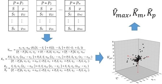
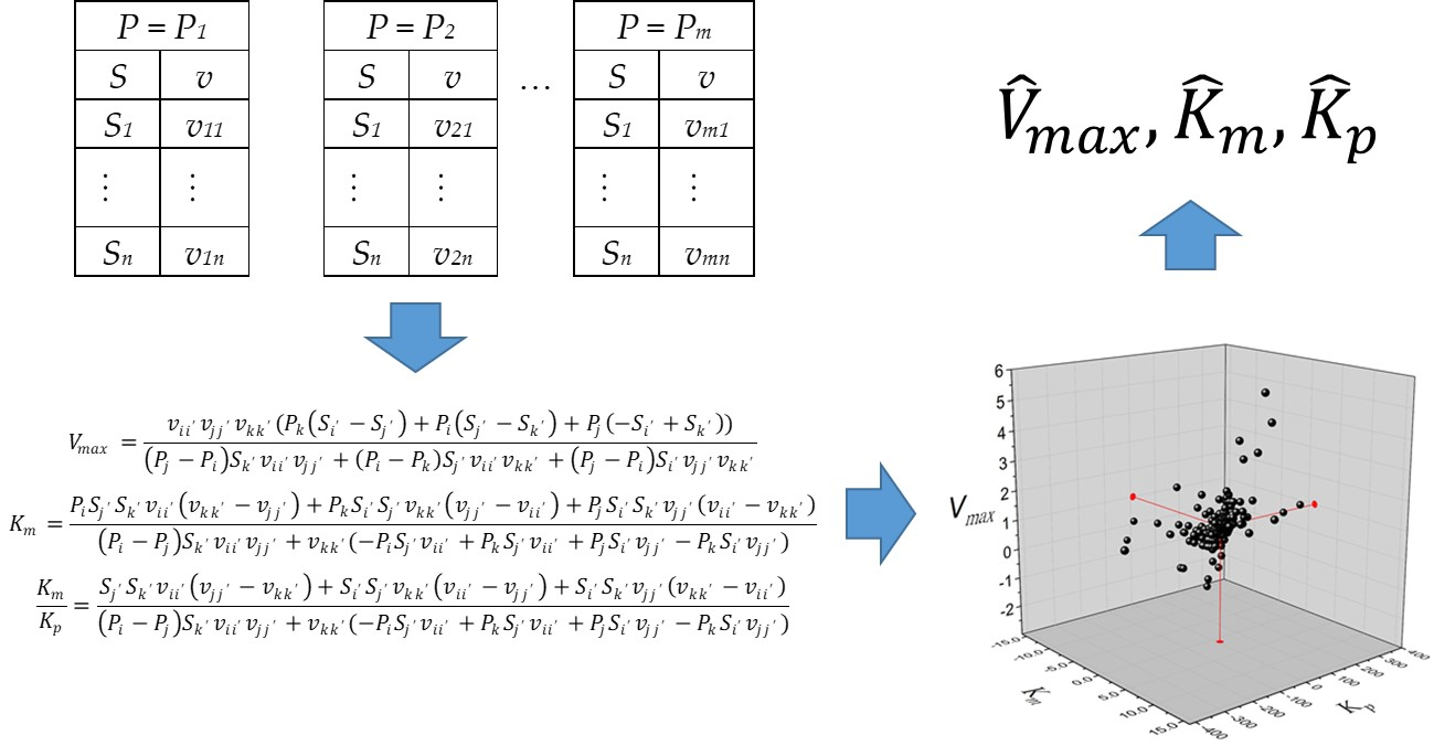
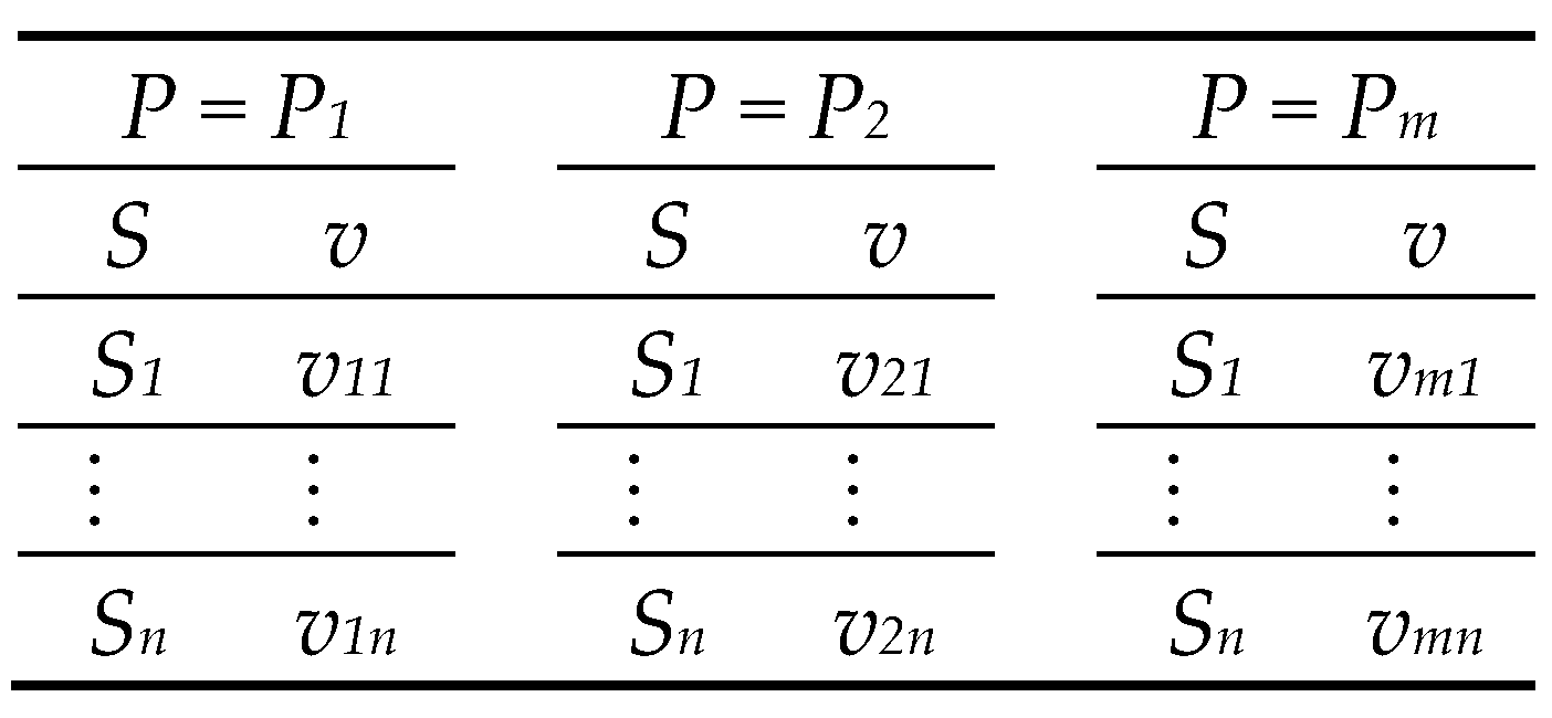
The experimental dataset required is traditionally used in the initial reaction rate method, which denotes a series of initial rates vs. substrate concentrations at constant product concentrations, as indicated in the scheme of Figure 1.
Equation (1) can be rearranged to Equation (3) in the following form:
v i j K m S j V m a x + v i j P i K m K p = v i j S j
The definition of vij is the rate of product concentration Pi and substrate concentration Sj. As the estimation of three parameters is required, three data pairs and three equations are needed to solve the matrix system in Equation (4).
( v i i S i v i i P i v j j S j v j j P j v k k S k v k k P k ) ( K m V m a x K m K p ) = ( v i i S i v j j S j v k k S k )
Likewise, the definition of vii’ = v(Pi, Si’), i.e., i values are between 1 and m (the number of product concentrations), and i’ values are between 1 and n (the number of substrate concentrations). Alternatively, the solution for Equation (4) is presented in Equation (5) in algebraic form.
V m a x = v i i v j j v k k ( P k ( S i S j ) + P i ( S j S k ) + P j ( S i + S k ) ) ( P j P i ) S k v i i v j j + ( P i P k ) S j v i i v k k + ( P j P i ) S i v j j v k k K m = P i S j S k v i i ( v k k v j j ) + P k S i S j v k k ( v j j v i i ) + P j S i S k v j j ( v i i v k k ) ( P i P j ) S k v i i v j j + v k k ( P i S j v i i + P k S j v i i + P j S i v j j P k S i v j j ) K m K p = S j S k v i i ( v j j v k k ) + S i S j v k k ( v i i v j j ) + S i S k v j j ( v k k v i i ) ( P i P j ) S k v i i v j j + v k k ( P i S j v i i + P k S j v i i + P j S i v j j P k S i v j j )
The rank of the matrix in Equation (4) must be 3 for the system to have a solution. For the case when three product concentrations are taken from the same set, Pi = Pj = Pk, the system has no solution because the rank of the resulting matrix is 2. This problem can be easily checked by observing the denominators of Equation (5) when replacing Pi, Pj, and Pk with the same value of product concentration. The strategy proposed to solve this system is to take at least two different values of product concentration. In this way, the total number of feasible data combinations will be calculated using Equation (6).
In consequence, calculations of the kinetic constants Vmax, Km, and Kp will be obtained from the combination of two P values from the same dataset, one P from a different one, and the combination of three different P values from three datasets. A list of Vmax, Km, and Kp values from the total combinations indicated in Equation (6) will be obtained. Finally, the estimators of Vmax, Km, and Kp correspond to the median values from the list.
( m · n 3 ) ( n 3 ) · m
This article aims to compare the quality of the kinetic constant estimations from the product inhibition equation between the DLP and the LS methods.

2. Results and Discussion

As in our previous article [
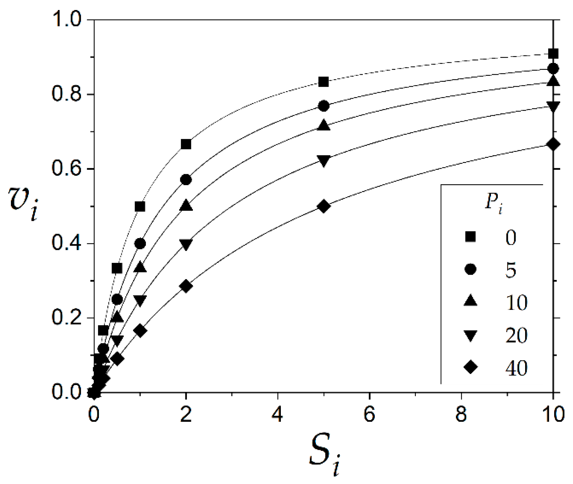
3], this problem consists of estimating three kinetic constants, but in this new case, three experimental variables will be used. Experimental data of initial rate perturbed with a random error of variance σ2 were simulated in a dataset of 1000 runs. The dataset, according to Table 1, considers the values of the kinetic constants 1, 1 and 10 for Vmax, Km, and Kp, respectively, and the initial rates vs. the substrate concentrations at different product concentrations were plotted in Figure 2.
These data were used to estimate the kinetic constants using the DLP and LS methods. An example of the dataset obtained for the values of the kinetic constants Vmax, Km, and Kp with a normal distribution of error and variance 0.01 is plotted in Figure 3.
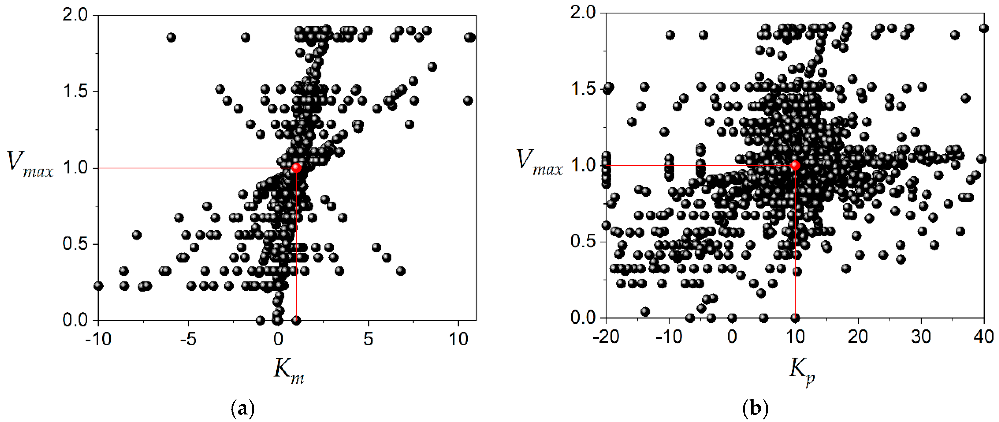
The number of kinetic constant values plotted in Figure 3 and Figure 4 was 6370. This amount of data was obtained avoiding the use of the same three product concentrations during the calculations with Equation (4). The dispersion of the data was enormous compared to the value of the kinetic constant, as can be observed in Figure 4. This is a typical result of the application of the DLP method to the estimation of kinetic constants. This behavior can be observed in previous publications [1,3,9]. Many points were left out of the layers just for illustration purposes; however, the vast majority of data are inside of layers corresponding to 98%, 99% and 99% for Vmax, Km and Kp, respectively. In terms of dispersion, 56% of calculated Vmax values are in the range 0.95–1.05; 22% of calculated Km values are in the range 0.95–1.05 and 24% of calculated Kp values are in the range 9.5–10.5. The amount of data plotted in Figure 3 and Figure 4 was obtained to estimate the kinetic constants Vmax, Km, and Kp by calculating the median for each of them. This is the procedure needed in routine experiments to determine the inhibition constant 
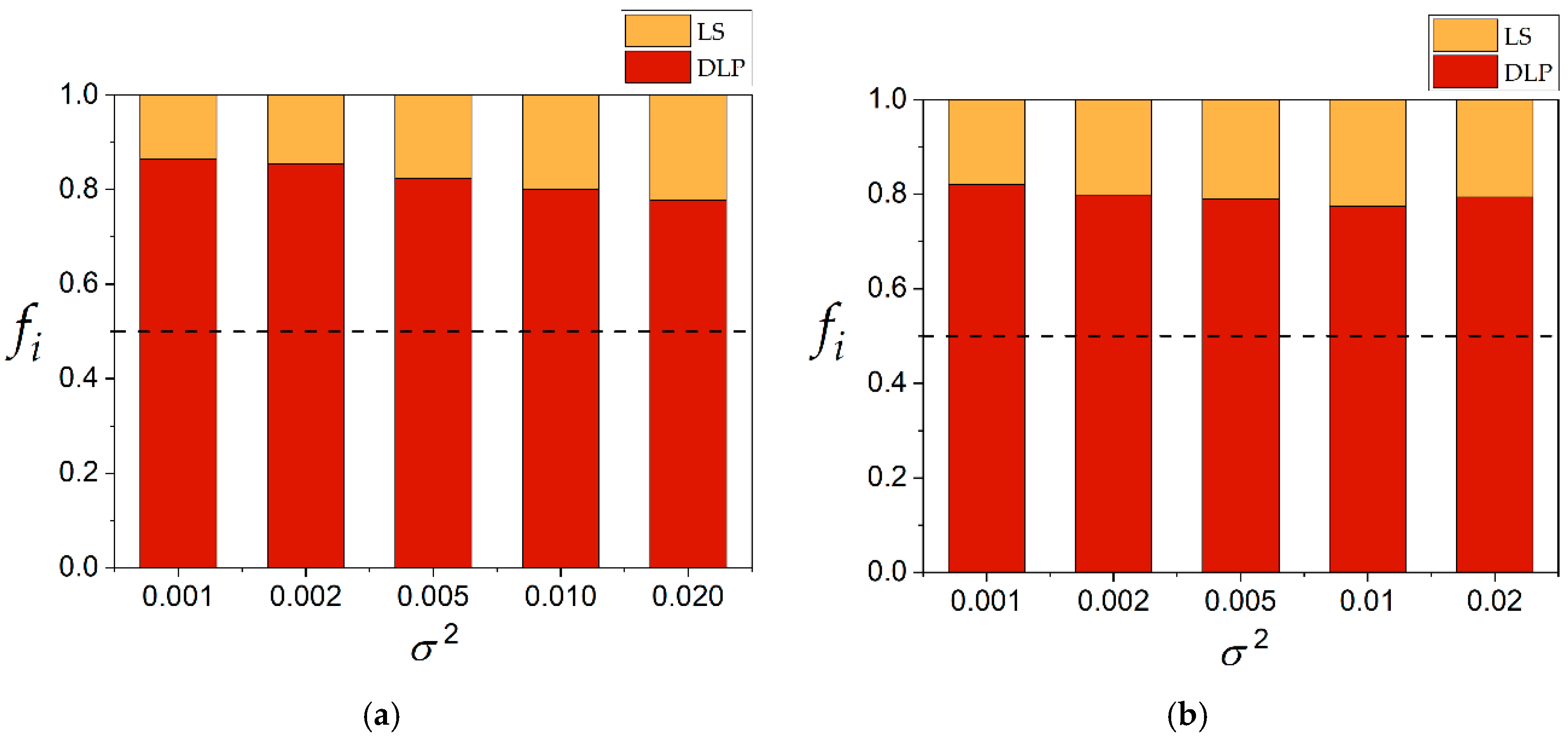
Kp. The statistical evaluation of DLP requires the repetition of this procedure to avoid bias and erroneous conclusions. A total of 1000 experimental runs were carried out to evaluate and compare the quality of the estimations between the DLP and the LS methods. A comparison of the lower values of the sum of squared residuals (SSR) between DLP and LS is plotted in Figure 5. The DLP method obtained lower values of SSR for all the values of variance in the range from 0.001 to 0.020 when both procedures—calculation of the median of Km/Kp and the median of Kp—were carried out. The calculation of the median of Km/Kp was slightly superior for almost all variances explored. For example, at variance 0.010, the calculation of the median of Km/Kp obtained a frequency of 0.8 compared to 0.78 for calculation of the median of 
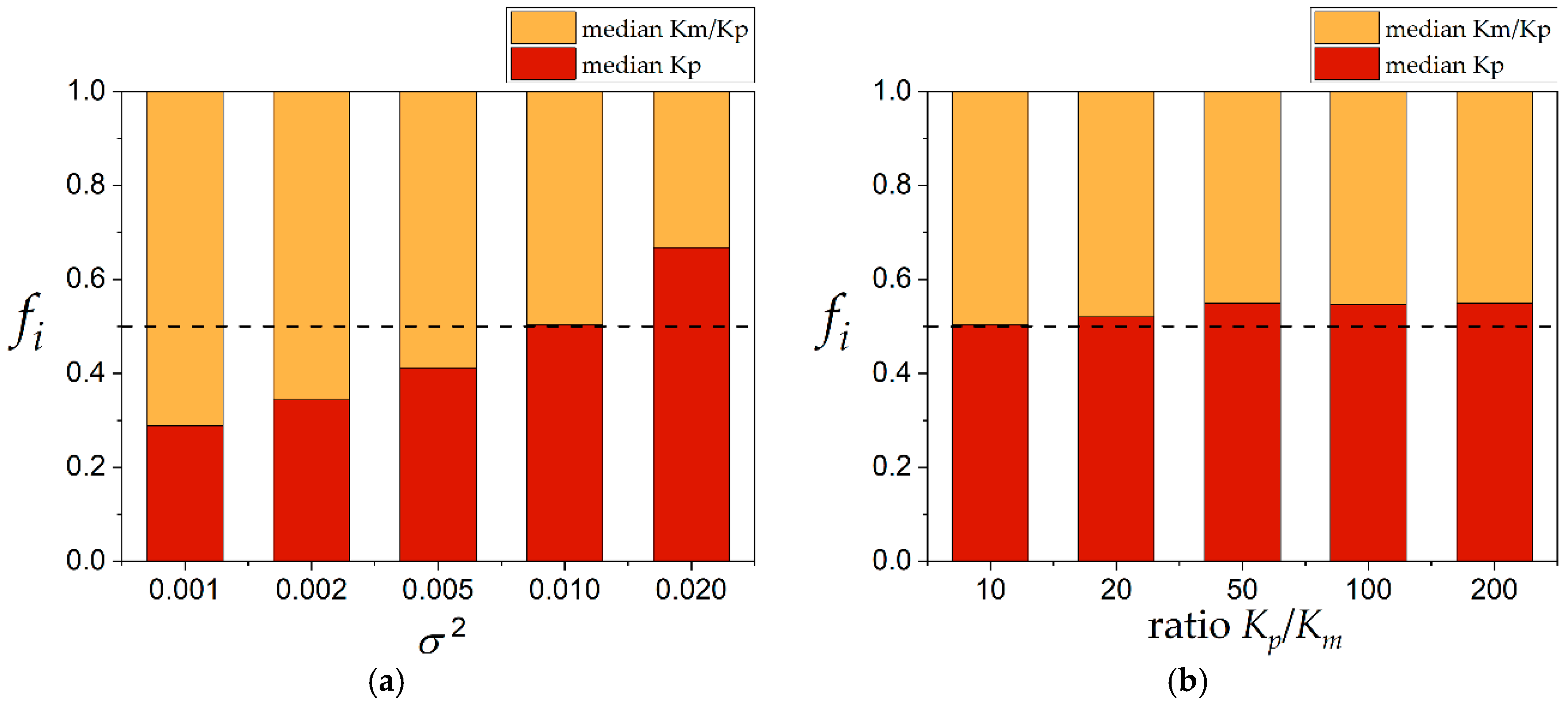
Kp. This was not significant to conclude that one procedure was better than the other. However, when both calculations were compared regarding the SSR between them, the result depended on the variance, as shown in Figure 6a. The calculation of the median of Km/Kp obtained a lower SSR at variance values lower than 0.010. The calculation of the median of Kp offered lower values of SSR at variances higher than 0.010. The effect of the ratio Kp/Km was slightly superior to the calculation of the median of Kp, as shown in Figure 6b. However, this was not significantly different. In consequence, which procedure is better, in terms of the SSR, depends on the experimental error.
The relative error of the estimated kinetic constants by LS and DLP methods was plotted for 1000 experimental runs in 
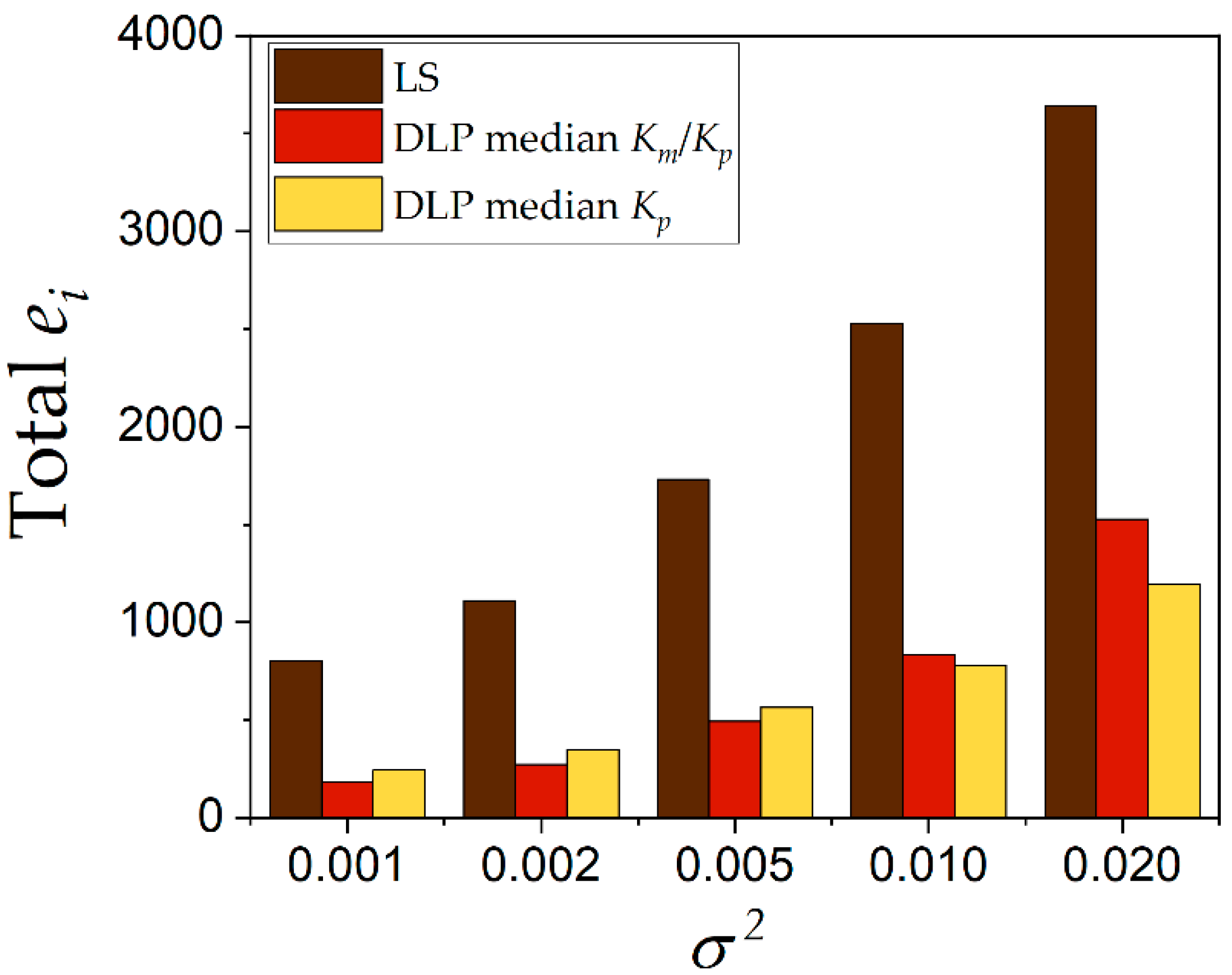
Figure 7. The DLP always resulted in a lower accumulation of relative error during estimations of the three kinetic constants. The product inhibition constant Kp accumulated the highest relative error when estimated by both LS and DLP methods. However, the accumulated relative error was less than half with DLP compared to LS. This result shows that DLP is a very accurate method to estimate the competitive inhibition constant. The product inhibition constant Kp estimated with DLP method accumulated a lower relative error than the LS method even at higher variance σ2 (experimental error), as shown in Figure 8. The behavior patterns of both the median of Km/Kp and the median of Kp were repeated. The median of Km/Kp was slightly more accurate at variances lower than 0.010. At higher values, the median of Kp was more accurate.
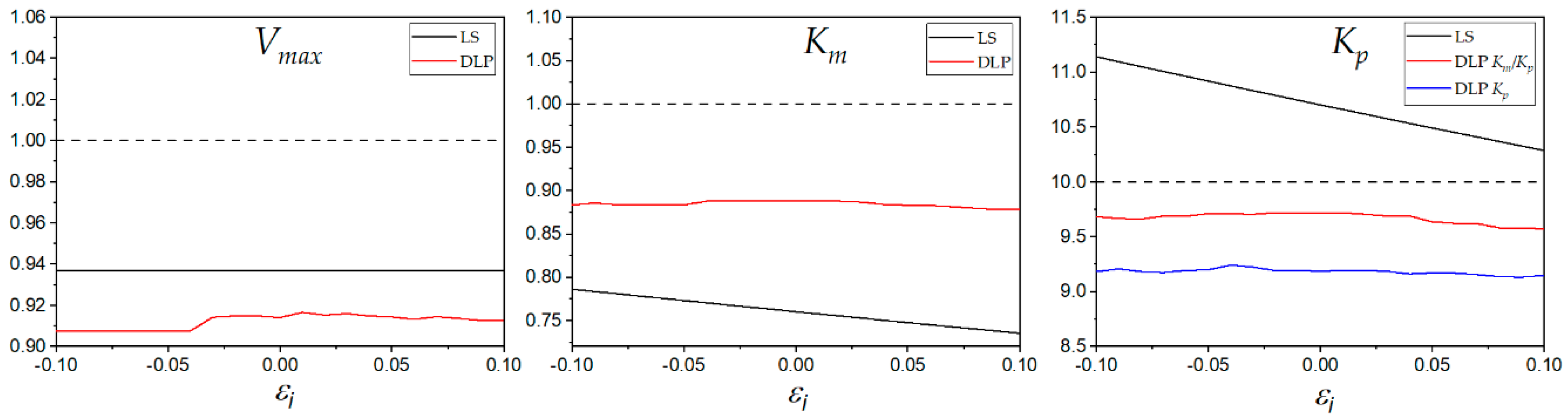
The effect of outliers was analyzed by adding fixed error values to the initial rate v34 (S = 1; P = 10). The added error ranged from −0.01 to +0.01. The results are shown in Figure 9. The estimated values of Vmax by LS were constant due to an artifact of the estimation method. The estimated Vmax was obtained by choosing the highest value from the five non-linear regressions corresponding to the five datasets of product concentrations. The error was added to the initial rate value corresponding to the third dataset of product concentration; in consequence, the highest value of Vmax was not perturbed, and it was always the same value. The DLP method estimated Km and the Kp with more accuracy and with less perturbation than the LS method. Although the LS method estimated 
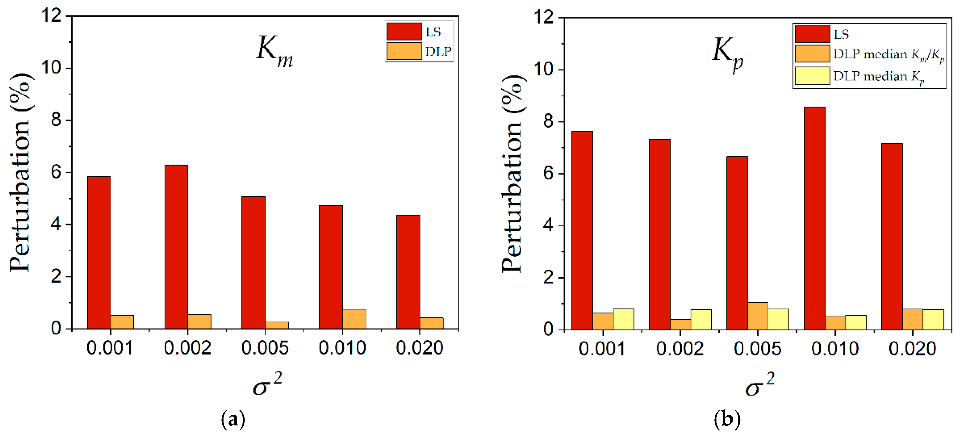
Kp with more accuracy at some high positive values of fixed error, the results clearly showed that DLP was more robust than the LS method. The perturbation generated by the added error is plotted in Figure 10. The perturbation of Vmax was omitted due to the artifact during its estimation by the LS method. The results indicated that the estimation of kinetic constants Km and Kp was much less perturbed when the DLP method was used. Almost all the perturbations were maintained below 1%, compared to the LS method, where perturbations were in the range from 4% to 8%.
The DLP method exhibited the same pattern of behavior than that observed during application to the uncompetitive inhibition equation [3]. Lower SSR and estimation errors compared to the LS method were observed during estimations of the competitive inhibition constant. Again, the DLP method demonstrated accuracy and robustness during the estimation of kinetic constants. The possibility of using the DLP method to estimate inhibition constants in pharmaceutical and biotechnological studies was demonstrated. The performance of the DLP method applied to the competitive inhibition equation was different compared to the application of the substrate-uncompetitive inhibition equation previously studied. The addition of a variable product concentration caused mathematical indetermination during the calculations. The problem was overcome by avoiding using the same three product concentrations in Equations (4) and (5). This obligated a reduction in the number of combinations from 6545 to 6370, where 175 combinations resulted in the indetermination of the matrix (Equation (4)). Another difference is the dependence of Kp on the value of Km, which can be observed in Equation (5), where the calculation consisted of the Km/Kp value, and Kp was calculated after obtaining Km. A significant implication of this is the transmission of the Km error to Kp. Interestingly, based on the observations, this effect was not important. In general, the estimation of Kp by DLP was more accurate and robust than estimation by the LS method. The application of DLP to the uncompetitive inhibition equation exhibited a higher accuracy just in some cases compared to the LS method. In terms of robustness, the DLP was highly superior to the LS method. Presently, in this study, a higher superiority in terms of accuracy and robustness was observed. Despite the higher complexity of the competitive inhibition equation, requiring one more independent variable than the substrate-uncompetitive inhibition equation, the results were better. The transmission of error from Km to Kp could be the key. This error is surely amplified when transmitted from one constant to another, and based on the observations, the effect was better softened by DLP compared to the LS method.
As Cornish-Bowden and Endrenyi commented [10], the median method cannot readily be generalized to equations of more than two parameters. This sentence became true when we found a mathematical issue during the application of the DLP to the product’s inhibition equation, where an indeterminate system of equations (Equation (5)) is generated when the same value for the product concentration was used. However, this problem can be solved by selecting the proper combination of data. We, again, demonstrated that DLP can be applied to equations with more than two parameters. Presently, we also demonstrated the application to equations with more than two variables.
We conclude that the DLP method is better than the LS method to estimate the product’s competitive inhibition constant in terms of accuracy and robustness. We now count on a new tool to estimate the product-competitive inhibition constant with reliable results.

3. Method

3.1. Experimental Design

The set of substrate and product concentrations was designed by first setting the real values of kinetic constants Vmax, Km, and Kp. The chosen values were 1 for Vmax and Km, and five different Kp values, including 10, 20, 50, 100 and 200, to study the effect on the estimation of the kinetic constants. These values correspond to the dimensionless kinetic constants in the case of Vmax and Km. Dimensionless Vmax is the limit of S/(S + Km) when S tends to infinity. Dimensionless Km is obtained when the kinetic equation is written in the form S/Km/(S/Km + 1). In the case of Kp, the dimensionless value corresponds to Kp/Km. As indicated by Cornish-Bowden et al. [2,10], the unitary values of Vmax and Km involved no loss of generality because they finally depend on the units of measurement. The values of substrate and product concentrations are listed in Table 1, corresponding to n = 7 and m = 5, according to the nomenclature in the scheme of Figure 1.
The chosen values of substrate concentrations were based on their distribution around the Km value from 0.1 Km to 10 Km, with three values below Km and three values above Km, as recommended by Cornish-Bowden [11]. In the case of product concentrations, the choice was based on a Kp value-centered distribution. The experimental design consisted of 35 reaction rates (vij), which were calculated using the product-competitive inhibition equation (Equation (1)) assigning relative errors from a normal population of error εi with variance σ2 (Equation (7)) to simulate the experimental error.
v i j = V m a x S i j K m + S i j + K m K p P j ( 1 + ε i )
The calculated reaction rates (vij) were used as experimental values to estimate the kinetic constants Vmax, Km, and Kp. The estimations were carried out by DLP, using Equation (4), and by the LS method. The number of possible combinations of three initial rate values (vij) to calculate the kinetic constants Vmax, Km, and Kp was 6370, according to Equations (4) and (5). The median for each kinetic constant was obtained from this list. This procedure corresponded to one experiment to calculate the estimators of the kinetic constants, which is equivalent to an empirical procedure based on the initial rates method. A total of 1000 experiments were run to compare the accuracy of both methods and the quality of parameter estimations. An algorithm was written in Python software to perform all the calculations presented in this article. The algorithm can be downloaded from the repository indicated in the Supplementary Material. Estimation of Kp was carried out by two optional procedures: (i) calculating Km/Kp for each of the 1000 experiments, calculating the median for Km/Kp, and finally obtaining the estimated Kp using the corresponding Km value, and (ii) calculating the Kp for each of the 1000 experiments and calculating the median of Kp (see Equation (5)). In the case of the LS method, a non-linear regression was applied to Equation (8), where the apparent Km ( K m a p p ) was estimated. According to the experimental design, five values of Vmax and K m a p p were obtained, one for each product concentration. As Vmax is not affected by competitive inhibition, a higher value was chosen as the estimated Vmax through the LS method. The K m a p p values were plotted against the product concentrations in a secondary plot, and the values of Km and Kp were obtained by linear regression of Equation (9).
v = V m a x S K m a p p + S
K m a p p = K m + K m K p P
The effect of the Kp/Km ratio was also evaluated. The values of Kp considered were 10, 20, 50, 100, and 200. The Kp/Km ratios corresponded to the same values, considering that Km was 1. As the values of Kp were modified, the experimental values of product concentration (P) were changed to maintain the same values of apparent Km, according to Equation (9), among the different datasets to avoid negative effects in the experimental design.

3.2. Accuracy Test

The sum of squared residuals (SSR) was calculated for each of the 1000 experiments for both methods, DLP and LS, to evaluate their accuracies, according to Equation (10).
S S R = i = 1 n ( v i v ^ i )
where v i is the ith value of the experimental rate (Equation (7)), and v ^ i is the ith value of the predicted rate calculated according to Equation (1). The relative error (ei) from the difference between the real ( θ ) and the estimated value ( θ ^ ) was calculated for all kinetic constants according to Equation (11).
e i = | θ ^ θ θ |
The number of experiments (out of 1000) in which the LS resulted in a lower SSR and ei was calculated and compared with DLP for different values of the variance σ2 for error εi.

3.3. Effect of Outliers

The sensitivity of both methods to outliers was tested by changing the initial rate value v34 from Table 1. This value corresponds to the substrate concentration equal to Km and the product concentration equal to Kp. The initial rate v34 was changed by varying fixed values of εi from −0.1 to +0.1. The rest of the experimental initial rates were calculated as mentioned above using Equation (6) with random εi with σ2 = 0.01. The perturbation generated on the estimated constant was calculated according to Equation (12).
% P e r t u r b a t i o n = θ ^ u θ ^ l θ · 100
where θ ^ u and θ ^ l are the upper and lower estimated values of the real constant θ in the range of the fixed error.

Supplementary Materials

The following are available online at https://github.com/bastiansepulveda/Inhibation-Equation-by-Product-Algorithms.git, algorithms for the analysis of DLP applied to the product’s competitive inhibition equation.

Author Contributions

Conceptualization, P.L.V. and B.S.; methodology, P.L.V., B.S. and D.G.; software, D.G. and B.S.; validation, P.L.V., D.G., B.S. and C.A.-C.; formal analysis, P.L.V. and C.A.-C.; writing—original draft preparation, P.L.V. and C.A.-C. All authors have read and agreed to the published version of the manuscript.

Funding

This research received no external funding.

Acknowledgments

Pedro Valencia would like to thank Pedro Gajardo for the opportunity of presenting the direct linear plot problem in his class Laboratory of Modeling.

Conflicts of Interest

The authors declare no conflict of interest.

References

  1. Eisenthal, R.; Cornish-Bowden, A. The direct linear plot: A new graphical procedure for estimating enzyme kinetic parameters. Biochem. J. 1974, 139, 715–720. [Google Scholar] [CrossRef] [PubMed]
  2. Cornish-Bowden, A.; Eisenthal, R. Statistical considerations in the estimation of enzyme kinetic parameters by the direct plot and other methods. Biochem. J. 1974, 139, 721–730. [Google Scholar] [CrossRef] [PubMed] [Green Version]
  3. Valencia, P.L.; Astudillo-Castro, C.; Gajardo, D.; Flores, S. Application of the median method to estimate the kinetic constants of the substrate uncompetitive inhibition equation. J. Theor. Biol. 2017, 418, 122–128. [Google Scholar] [CrossRef] [PubMed]
  4. Airas, R.K. The Computation of Hyperbolic Dependences in Enzyme Kinetics. Biochem. J. 1976, 155, 449–452. [Google Scholar] [CrossRef] [PubMed] [Green Version]
  5. Porter, W.R.; Trager, W.F. Improved Non-Parametric Statistical Methods for the Estimation of Michaelis-Menten Kinetic Parameters by the Direct Linear Plot. Biochem. J. 1977, 161, 293–302. [Google Scholar] [CrossRef] [PubMed] [Green Version]
  6. Reading, C.; Hepburn, P. The Inhibition of Staphylococcal Beta-Lactamase by Clavulanic Acid. Biochem. J. 1979, 179, 67–76. [Google Scholar] [CrossRef] [PubMed]
  7. Bialojan, C.; Takai, A. Inhibitory Effect of a Marine-Sponge Toxin, Okadaic Acid, on Protein Phosphatases. Specificity and Kinetics. Biochem. J. 1988, 256, 283–290. [Google Scholar] [CrossRef] [PubMed]
  8. Takai, A.; Mieskes, G. Inhibitory Effect of Okadaic Acid on the P-Nitrophenyl Phosphate Phosphatase Activity of Protein Phosphatases. Biochem. J. 1991, 275, 233–239. [Google Scholar] [CrossRef] [PubMed] [Green Version]
  9. Cornish-Bowden, A.; Eisenthal, R. Estimation of Michaelis constant and maximum velocity from the direct linear plot. Biochim. Biophys. Acta 1978, 523, 268–272. [Google Scholar] [CrossRef]
  10. Cornish-Bowden, A.; Endrenyi, L. Robust regression of enzyme kinetic data. Biochem. J. 1986, 234, 21–29. [Google Scholar] [CrossRef] [PubMed] [Green Version]
  11. Cornish-Bowden, A. Fundamentals of Enzyme Kinetics, 4th ed.; Wiley-VCH Verlag & Co: Weinheim, Germany, 2012. [Google Scholar]
Figure 1. Scheme of the traditional experimental design based on the initial reaction rate method to estimate inhibition constants in enzyme kinetics.
Catalysts 10 00853 g001
Figure 2. Initial reaction rates vs. substrate concentration for the different product concentrations according to the experimental design presented in Table 1. Data plotted without error for illustration purposes. The kinetic constant values for Vmax, Km, and Kp are 1, 1, and 10, respectively.
Catalysts 10 00853 g002
Figure 3. Three-dimensional projection of the direct linear plot (DLP) values obtained according to the experimental design presented in Table 1. The kinetic constant values for Vmax, Km, and Kp are 1, 1, and 10, respectively. The median of each kinetic constant (red dots) is projected on the planes. Some data are outside of the layers for illustration purposes only.
Catalysts 10 00853 g003
Figure 4. DLP for the competitive inhibition equation to estimate Vmax, Km, and Kp with real values of 1, 1, and 10, respectively, considering a normal distribution of error with variance 0.01. (a) Plot of Vmax vs. Km; (b) plot of Vmax vs. Kp. The median values (red dots) are projected on each axis. Some data are outside of layers for illustration purposes only. Data inside of layers is 98%, 99% and 99% for Vmax, Km and Kp, respectively.
Catalysts 10 00853 g004
Figure 5. Frequency (fi) of the lower sum of squared residuals (SSR) obtained between DLP and least-squares (LS) methods as a function of the variance (σ2) of the normal distribution of error (εi). The total number of experiments was 1000. (a) DLP applied to the median of Km/Kp; (b) DLP applied to the median of Kp. The dotted line represents the frequency 0.5, where both methods, LS and DLP, obtained the same statistical quality. The results showed that DLP obtained a lower SSR than LS approximately in 80% of the estimations.
Catalysts 10 00853 g005
Figure 6. Frequency (fi) of the lower SSR obtained between both the calculation of the median of Km/Kp and the median of Kp. (a) Results of frequency as a function of the variance (σ2) of the normal distribution of error (εi). (b) Results of frequency as a function of the ratio Km/Kp. The interpretation is the same as Figure 5.
Catalysts 10 00853 g006
Figure 7. Relative error (ei) for the estimations of kinetic constants Vmax, Km, and Kp by LS and DLP methods accumulated during iterations (i) of 1000 experimental runs with a normal distribution of error (εi) and variance (σ2) 0.010. The Kp was estimated by DLP using the median of Km/Kp (red line) and the median of Kp (blue line).
Catalysts 10 00853 g007
Figure 8. Total relative error (ei) accumulated for estimations of the product inhibition constants Kp by LS and DLP methods after 1000 experimental runs plotted against variance (σ2) of the normal distribution of error (εi). The Kp was estimated by DLP using the median of Km/Kp (red bars) and the median of Kp (yellow bars).
Catalysts 10 00853 g008
Figure 9. Effect of the fixed error added to the initial rate v34 on the estimated values of the kinetic constants Vmax, Km, and Kp by LS and DLP methods. Real kinetic constant value (dotted line), estimated values by LS (black line) and DLP (red and blue lines). The Kp was estimated by DLP using the median of Km/Kp (red line) and the median of Kp (blue line).
Catalysts 10 00853 g009
Figure 10. Perturbation percentage on the estimations of Km and Kp by LS and DLP methods caused by adding fixed error to the initial rate v34 at different values of variance (σ2). (a) Km. (b) Kp. The perturbation corresponds to the difference between the minimum and the maximum value obtained respect to the original value of the kinetic constant (Equation (12)).
Catalysts 10 00853 g010
Table 1. Experimental design of substrate and product concentrations to calculate initial reaction rates.
P1 = 0P2 = 0.5KpP3 = KpP4 = 2KpP5 = 4Kp
SvSvSvSvSv
0.1v110.1v210.1v310.1v410.1v51
0.2v120.2v220.2v320.2v420.2v52
0.5v130.5v230.5v330.5v430.5v53
1.0v141.0v241.0v341.0v441.0v54
2.0v152.0v252.0v352.0v452.0v55
5.0v165.0v265.0v365.0v465.0v56
10.0v1710.0v2710.0v3710.0v4710.0v57

