Article

Ranking Supply Function and Cournot Equilibria in a Differentiated Product Duopoly with Demand Uncertainty

Yildiz 88 Sitesi, Alacaatli Mahallesi, Cankaya, Ankara 06810, Turkey
Games 2018, 9(3), 60; https://doi.org/10.3390/g9030060
Submission received: 26 June 2018 / Revised: 7 August 2018 / Accepted: 18 August 2018 / Published: 21 August 2018
(This article belongs to the Special Issue Games and Industrial Organization)

Abstract

:
In this paper, we provide a welfare ranking for the equilibria of the supply function and quantity competitions in a differentiated product duopoly with demand uncertainty. We prove that the expected consumer surplus is always higher under the supply function competition, irrespective of whether the (duopolistic) products are substitutes, complements, or independent. Numerical simulations suggest that if the products are either complements or independent, or if they have an extremely low degree of substitution, then the supply function competition can always be Pareto superior to the quantity competition in terms of the producers’ and consumers’ welfares. Moreover, if the degree of product substitution is not extremely low, then the supply function competition can be Pareto superior to the quantity competition if and only if the size of the demand uncertainty is sufficiently large to exceed a critical level. We find that this critical level of demand uncertainty becomes higher when the duopolistic products are less differentiated. Additionally, this critical level is nonincreasing both in the marginal cost of producing a unit output and in the own-price sensitivity of each inverse demand curve when all other parameters are fixed. Our results imply that in electricity markets with differentiated products, the regulators should not intervene to impose the quantity competition in favor of the supply function competition unless the degree of product substitution is sufficiently high and the predicted demand fluctuations are sufficiently small.

1. Introduction

The supply function competition that was originally developed by Grossman (1981) [1] could find applications in oligopolistic industries only after Klemperer and Meyer (1989) [2], who eliminated the problems with the multiplicity of supply function equilibria by introducing an exogenous uncertainty about the demand functions faced by oligopolists. The best-known application has arisen from the deregulated electricity markets, for which the supply function competition has been found to model the strategic interplay among power generators more successfully than the price competition of Bertrand (1883) [3] and the quantity competition of Cournot (1838) [4] (see, e.g., Green and Newbery (1992) [5], Rudkevich and Duckworth (1998) [6], and Rudkevich et al. [7] (1998)). Since Klemperer and Meyer (1989) [2], an appraisal of the supply function competition in terms of the expected welfares of producers and/or consumers has been made both in the absence and in the presence of demand uncertainty.
In the absence of demand uncertainty, the welfare analysis of Klemperer and Meyer (1989) [2] established the result that profits of oligopolistic producers under the supply function competition are intermediate between Bertrand [3] and Cournot [4] competition profits. This result was recently challenged by Delbono and Lambertini (2016) [8], who showed that with quadratic costs, price competition yields multiple equilibria, which can be separated into three groups depending upon whether the profits under the price competition are (i) above the profits under the quantity competition, (ii) below the profits under the supply function competition, or (iii) in between the profits under the quantity and supply function competitions. Delbono and Lambertini (2016) [8] also showed that at any price competition equilibrium within the first group mentioned above, the social welfare would be even lower than at the quantity competition equilibrium. On the other hand, Monden (2017) [9] showed that in a vertical market in which an upstream firm sequentially contracts with two downstream firms, the social welfare under the supply function competition may be lower than that under the quantity and price competitions. In the literature, a number of works have also studied—under various settings—the supply function and quantity competitions in comparison. For instance, Ciarreta and Gutiérrez-Hita (2006) [10] investigated whether collusion in an infinitely lived oligopolistic industry is easier to sustain under the supply function or under the quantity competition. Their main result was that the supply function competition (the quantity competition) is the superior mode of competition to sustain collusive agreements if the number of oligopolistic firms is sufficiently low (sufficiently high and the slope of the demand curve is sufficiently low). More recently, Saglam (2018) [11] showed that in an oligopolistic industry with a homogeneous product and demand uncertainty, the supply function competition is always ex ante welfare superior to the quantity competition from the viewpoint of consumers independently of the size of the demand uncertainty. Saglam (2018) [11] also found that if the demand uncertainty in the industry is sufficiently large with respect to the number of firms, the size of the product markets, and the marginal cost of a unit output, then the supply function competition can also be ex ante more desirable for the producers. In this paper, we study the question of whether the results of Saglam (2018) [11] extend to the case of differentiated products. We believe that this question is important especially for the analysis of electricity markets, for which not only the supply function competition has a wide application, but the product differentiation, as recently argued in a comprehensive survey by Woo et al. (2014) [12], can also be considered a very meaningful concept.1
We answer our research question by borrowing from Singh and Vives (1984) [13] a duopolistic industry setting with product differentiation and demand uncertainty.2 For this setting, we characterize the unique and symmetric Nash (1950) [14] equilibrium obtained under the supply function and quantity competitions, and we show that the expected consumer surplus under the supply function competition is always higher than that under the quantity competition independently of the size of the demand uncertainty and any other attributes of the industry. Additionally, our numerical simulations suggest that if the duopolistic products are either complements or independent, or if they have an extremely low degree of substitution, then the supply function competition can always be Pareto superior to the quantity competition. However, if the degree of product substitution is not extremely low, then the expected producer profits under the supply function competition can be lower than those under the quantity competition in situations for which the size of the demand uncertainty is below a critical level. We find that this critical level of demand uncertainty becomes higher when the duopolistic products are less differentiated. Additionally, this critical level is nonincreasing both in the marginal cost of producing a unit output and in the own-price sensitivity of each inverse demand curve when all other parameters are fixed.
The rest of the paper is organized as follows: Section 2 introduces a duopoly model with differentiated products and demand uncertainty. Section 3 presents the results, and Section 4 concludes.

2. Model

By borrowing from Singh and Vives (1984) [13], we consider a duopolistic industry, in which each firm produces a differentiated product under demand uncertainty and faces a continuum of identical consumers. Each firm producing a quantity of output q 0 incurs the cost
C ( q ) = c q 2 / 2
with c > 0 . On the other hand, the representative consumer maximizes his/her surplus
U ( q 1 , q 2 ) i = 1 2 p i q i ,
where q i 0 denotes the quantity produced by firm i = 1 , 2 , and p i 0 denotes the price of its product. It is assumed that the utility function U is given by
U ( q 1 , q 2 ) = α ( q 1 + q 2 ) 1 2 ( β q 1 2 + 2 γ q 1 q 2 + β q 2 2 ) ,
where β > | γ | 0 . The products of the two firms are independent if γ = 0 , substitutes if γ > 0 , and complements if γ < 0 . The ratio γ / β measures the degree of product differentiation. Moreover, in the above function, α is a scalar random variable representing an ex ante unobservable shock to the utility of consumers. This shock variable is distributed with density f ( α ) that is strictly positive everywhere on the support [ 0 , ) . Given this density distribution, we let E [ α ] and σ ( α ) respectively denote the mean and the standard deviation of α .
Given Equations (2) and (3), the solution to the maximization problem of the representative consumer yields the inverse demands P i ( q i , q j ) , i = 1 , 2 satisfying
P i ( q i , q j ) = α β q i γ q j .
In the region of quantity space in which the prices p i and p j of firms i and j are nonnegative, the demand curve of firm i can then be derived as follows:
D i ( p i , p j ) = a b p i + g p j ,
where a = α / ( β + γ ) , b = β / ( β 2 γ 2 ) and g = γ / ( β 2 γ 2 ) . It is assumed that the form of the cost, demand, and inverse demand curves; the parameters c , β , γ , b , and g; and the density f ( α ) and its support are commonly known by both firms.

3. Results

For the industry described above, we characterize and analyze, in Section 3.1 and Section 3.2, the equilibria under the quantity and supply function competitions, respectively. Later, in Section 3.3, we make a welfare comparison between these two forms of competition for consumers and producers.

3.1. Quantity Competition

In this form of competition, firms set fixed quantities before production takes place, without knowing the realization of the demand shock. That is, a strategy for firm i = 1 , 2 is a nonnegative quantity of output, q i [ 0 , ) . Firms simultaneously determine their strategies to maximize their expected profits. We say that a pair of quantities q ^ 1 and q ^ 2 constitutes a Nash equilibrium if, for each i , j { 1 , 2 } with j i , the quantity q ^ i maximizes the expected profits of firm i when firm j sticks to the quantity q ^ j . That is, the quantity q ^ i solves
max q i 0 E P i ( q i , q ^ j ) q i c 2 q i 2 .
Proposition 1.
In the studied duopolistic industry with differentiated products and demand uncertainty, there exists a unique symmetric (Cournot) Nash equilibrium in quantities, where each firm chooses the quantity given by
q C = 1 2 β + γ + c E [ α ] .
Proof. 
Using Equation (4) at q j = q ^ j , the optimization problem in Equation (6) can be written as
max q i 0 E α β q i γ q ^ j q i c 2 q i 2 .
Differentiating Equation (8) with respect to q i , we obtain the first-order necessary condition
E [ α ] 2 β q i γ q ^ j c q i = 0 .
If the strategy pair ( q ^ i , q ^ j ) is a Nash equilibrium, then q i = q ^ i must satisfy the above first-order condition. Moreover, if this equilibrium is symmetric, we must have q ^ i = q ^ j q C . Inserting these into Equation (9), we obtain
q C = 1 2 β + γ + c E [ α ] .
Finally, for the problem in Equation (8), the second-order sufficient condition holds, as
2 E [ π i ( α ) ] ( q i ) 2 = 2 β c < 0 .
Thus, the choice of quantities ( q C , q C ) constitutes a Nash equilibrium. ☐
We note that using Equations (4) and (7), we can calculate the equilibrium price at any realization of α as follows:
p C ( α ) = P i ( q C , q C ) = α ( β + γ ) q C = α β + γ 2 β + γ + c E [ α ] .
Accordingly, given any α , the equilibrium profits of each firm become
π C ( α ) = p C ( α ) q C c 2 ( q C ) 2 = α q C ( β + γ ) ( q C ) 2 c 2 ( q C ) 2 = α 1 2 β + γ + c E [ α ] β + γ + c 2 1 2 β + γ + c 2 ( E [ α ] ) 2 .
It follows that the expected equilibrium profits of each firm are given by
E [ π C ( α ) ] = β + c 2 1 2 β + γ + c 2 ( E [ α ] ) 2 .
Corollary 1.
The expected producer profits E [ π C ( α ) ] are always decreasing in β, γ, and c.
Proof. 
Differentiating Equation (14) with respect to β , we obtain
E [ π C ( α ) ] β = 1 2 β + γ + c 2 γ 2 β c 2 β + γ + c ( E [ α ] ) 2 < 0 ,
as γ < β and c > 0 by assumption. Now, differentiating Equation (14) with respect to γ , we obtain
E [ π C ( α ) ] γ = 2 β + c 2 1 2 β + γ + c 3 ( E [ α ] ) 2 < 0 .
Finally, differentiating Equation (14) with respect to c yields
E [ π C ( α ) ] c = 1 2 β + γ + c 2 γ 2 β c 2 2 β + γ + c ( E [ α ] ) 2 < 0 ,
completing the proof. ☐
Now, we consider the welfare of consumers. Using Equations (2), (3), (7), and (12), we can calculate at any α the equilibrium consumer surplus as
C S C ( α ) = 2 α q C ( α ) ( β + γ ) q C ( α ) 2 2 p C ( α ) q C = ( β + γ ) ( q C ) 2 = β + γ 1 2 β + γ + c 2 ( E [ α ] ) 2 .
Because C S C ( α ) is independent of the realization of α , the expected consumer surplus E [ C S C ( α ) ] is equal to C S C ( α ) .
Corollary 2.
The expected consumer surplus E [ C S C ( α ) ] is always decreasing in c.
Proof. 
Because E [ C S C ( α ) ] = C S C ( α ) , we differentiate Equation (18) with respect to c to obtain
E [ C S C ( α ) ] c = 2 β + γ 1 2 β + γ + c 3 ( E [ α ] ) 2 < 0 ,
completing the proof. ☐
The effects of the parameters β and γ on the expected consumer surplus, E [ C S C ( α ) ] , are more involved. As we show below, E [ C S C ( α ) ] is decreasing (increasing) in β and γ if and only if the value of c, the marginal cost of producing a unit output, is sufficiently small (large).
Corollary 3.
The expected consumer surplus E [ C S C ( α ) ] is decreasing in β if and only if c < 2 β + 3 γ and is decreasing in γ if and only if c < γ .
Proof. 
Because E [ C S C ( α ) ] = C S C ( α ) , we differentiate Equation (18) with respect to β to obtain
E [ C S C ( α ) ] β = 1 2 β + γ + c 2 c 2 β 3 γ 2 β + γ + c ( E [ α ] ) 2 .
Clearly, E [ C S C ( α ) ] / β < 0 if and only if c < 2 β + 3 γ . Now, differentiating Equation (18) with respect to γ , we obtain
E [ C S C ( α ) ] γ = 1 2 β + γ + c 2 c γ 2 β + γ + c ( E [ α ] ) 2 .
Thus, E [ C S C ( α ) ] / γ < 0 if and only if c < γ . ☐
The above corollary implies that the expected consumer surplus E [ C S C ( α ) ] is decreasing in γ if and only if the duopolistic products are substitutes, that is, γ > 0 .

3.2. Supply Function Competition

Here, firms are assumed to simultaneously specify supply functions without observing the realization of the demand shock α . The supply function of each firm maps a nonnegative price for its product into a nonnegative quantity of output.
Proposition 2. (Klemperer and Meyer (1989) [2]).
In the studied duopolistic industry with differentiated products and demand uncertainty, there exists a unique and symmetric Nash equilibrium in supply functions whereby each firm chooses the supply function given by
S S F ( p ) = ξ p ,
where
ξ = ( b 2 g 2 ) b + b 2 g 2 b 2 + 4 c b 2 g 2 b 1 + 1 b c 2 1 + 1 b c .
Proof. 
For the case of β > γ > 0 (or equivalently b > g > 0 ), the proof is available in pages 1267–1269 of Klemperer and Meyer (1989) [2]. This proof is also valid for the case of β > 0 γ (or equivalently b > 0 g ). ☐
We note that given the equilibrium supply functions in Equations (22) and (23) and given any realization of the demand shock α , we can calculate the market clearing price p S F ( α ) using the market clearing condition in any market i = 1 , 2 , that is, S S F ( p S F ( α ) ) = D i ( p S F ( α ) , p S F ( α ) ) , implying ξ p S F ( α ) ( α ) = a + ( g b ) p S F ( α ) , and further implying
p S F ( α ) = a b g + ξ = α 1 + ξ ( β + γ ) .
Then, given Equation (24), it follows from Equation (22) that under the supply function competition, each firm must produce the equilibrium quantity
q S F ( α ) = ξ α 1 + ξ ( β + γ ) .
Using Equations (24) and (25), the equilibrium profits of each firm can be calculated as
π S F ( α ) = p S F ( α ) q S F ( α ) c 2 q S F ( α ) 2 = 1 ξ c 2 ξ α 1 + ξ ( β + γ ) 2 .
Hence, the expected equilibrium profits of each firm become
E [ π S F ( α ) ] = 1 ξ c 2 ξ 1 + ξ ( β + γ ) 2 E [ α 2 ] .
On the other hand, using Equations (2), (3), (24), and (25), we can calculate at any α the equilibrium consumer surplus as
C S S F ( α ) = 2 α q S F ( α ) ( β + γ ) q S F ( α ) 2 2 ξ q S F ( α ) 2 = ( β + γ ) q S F ( α ) 2 = ( β + γ ) ξ α 1 + ξ ( β + γ ) 2
and the expected equilibrium consumer surplus as
E [ C S S F ( α ) ] = ( β + γ ) ξ 1 + ξ ( β + γ ) 2 E [ α 2 ] .
We observe that under the supply function competition, both the expected producer profits and the expected consumer surplus depend on E [ α 2 ] . This term can be expressed as
E [ α 2 ] = 1 + η 2 E [ α ] 2 ,
where
η = σ ( α ) E [ α ] .
We note that η , called the coefficient of variation, is a unitless measure of the size of the demand uncertainty. Keeping E [ α ] fixed, we observe that the larger the coefficient η , or equivalently σ ( α ) , the greater the expected producer profits in Equation (27) and the expected consumer surplus in Equation (29). That is, the size of the demand uncertainty positively affects the expected welfares of both producers and consumers under the supply function competition.
Now, we investigate the welfare effects of the parameter c measuring the marginal cost of producing a unit output. For this, we have to first find how the slope of the equilibrium supply functions is affected by c. We note that using ( b 2 g 2 ) / b = 1 / β and 1 / b = ( β 2 γ 2 ) / β , Equation (23) can be rewritten as
ξ = 1 + 1 + 4 c β + β 2 γ 2 c 2 β + β 2 γ 2 c .
Studying Equation (32), we observe the following.
Lemma 1.
The slope of the equilibrium supply function, ξ, is always decreasing in c.
Proof. 
We note that Equation (32) implies
1 ξ = 2 ( β c + β 2 γ 2 ) c + c 2 + 4 β c + 4 ( β 2 γ 2 ) .
Then, we can compute
c 1 ξ = 2 β c + c 2 + 4 β c + 4 ( β 2 γ 2 ) 2 ( β c + β 2 γ 2 ) 1 + c + 2 β c 2 + 4 β c + 4 ( β 2 γ 2 ) c + c 2 + 4 β c + 4 ( β 2 γ 2 ) 2 = ( β 2 γ 2 ) 4 β + 2 c 2 + 4 β c + 4 ( β 2 γ 2 ) + 2 c β 2 + 2 c γ 2 c 2 + 4 β c + 4 ( β 2 γ 2 ) c + c 2 + 4 β c + 4 ( β 2 γ 2 ) 2 ,
which is always positive, implying that 1 / ξ is always increasing in c. Therefore, ξ is always decreasing in c. ☐
Using Lemma 1, we can also show that under the supply function competition, the marginal cost of a unit output always has a negative impact on both the expected producer profits and the expected consumer surplus.
Corollary 4.
E [ π S F ( α ) ] and E [ C S S F ( α ) ] are always decreasing in c.
Proof. 
Differentiating Equation (27) with respect to c yields
E [ π S F ( α ) ] c = 1 2 1 1 ξ + ( β + γ ) 2 E [ α 2 ] 2 1 ξ c 2 1 1 ξ + ( β + γ ) 3 E [ α 2 ] c 1 ξ .
Lemma 1 implies that E [ π S F ( α ) ] c < 0 . On the other hand, differentiating Equation (29) yields
E [ C S S F ( α ) ] c = 2 ( β + γ ) 1 1 ξ + ( β + γ ) 3 E [ α 2 ] c 1 ξ .
Now, Lemma 1 implies that E [ C S S F ( α ) ] c < 0 . ☐
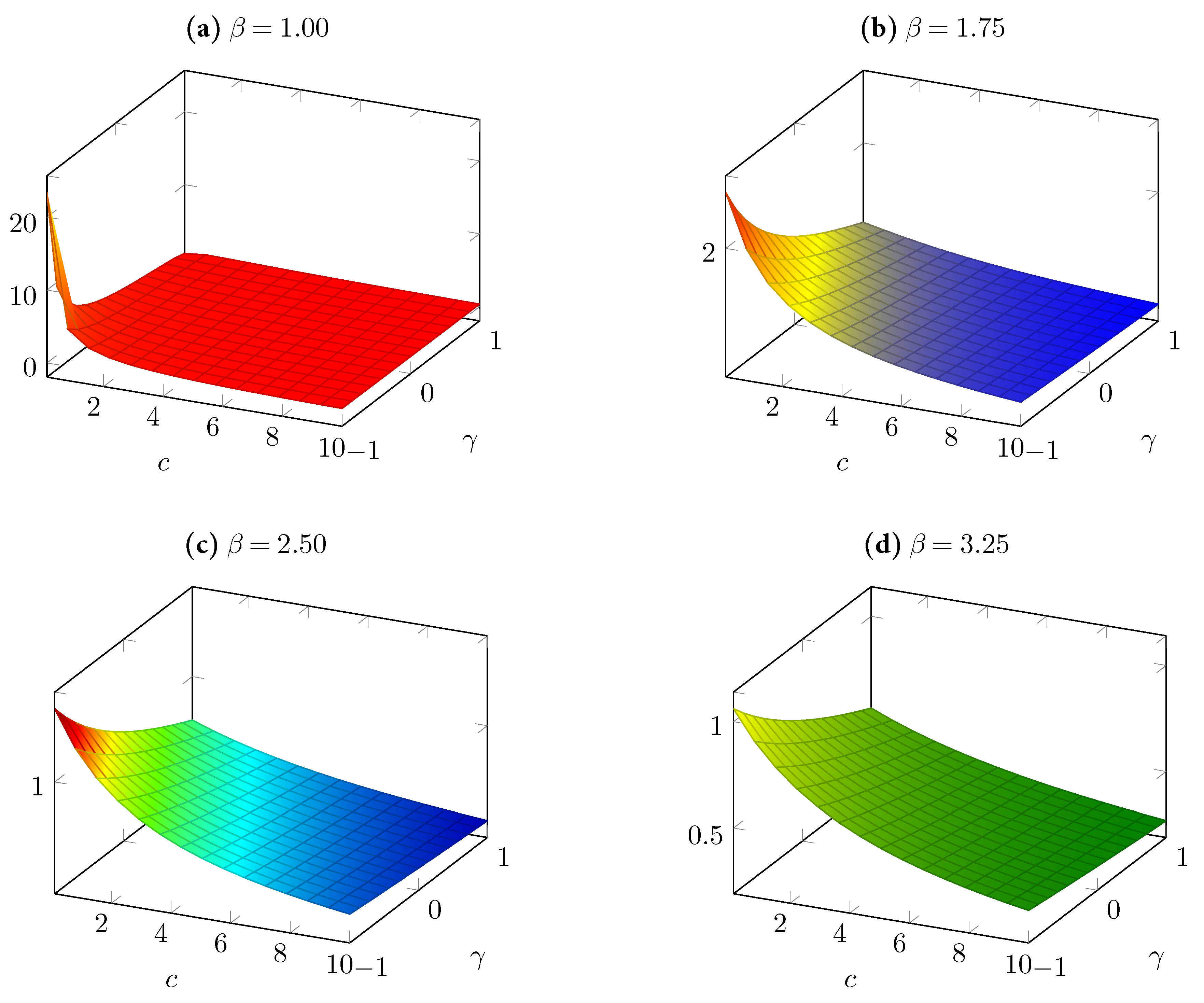
As we were not successful in analytically studying the dependence of E [ π S F ( α ) ] and E [ C S S F ( α ) ] on β and γ in their defined domains, we tried to infer these dependencies with the help of some numerical simulations, which we illustrate in Figure 1 and Figure 2. We note that the four graphs in each figure correspond to the four values of β in the set { 1.00 , 1.75 , 2.50 , 3.25 } . In each of these graphs, we considered 15 sample points for c between 0.1 and 10.00 and 15 sample points for γ between −1.00 and 1.00.
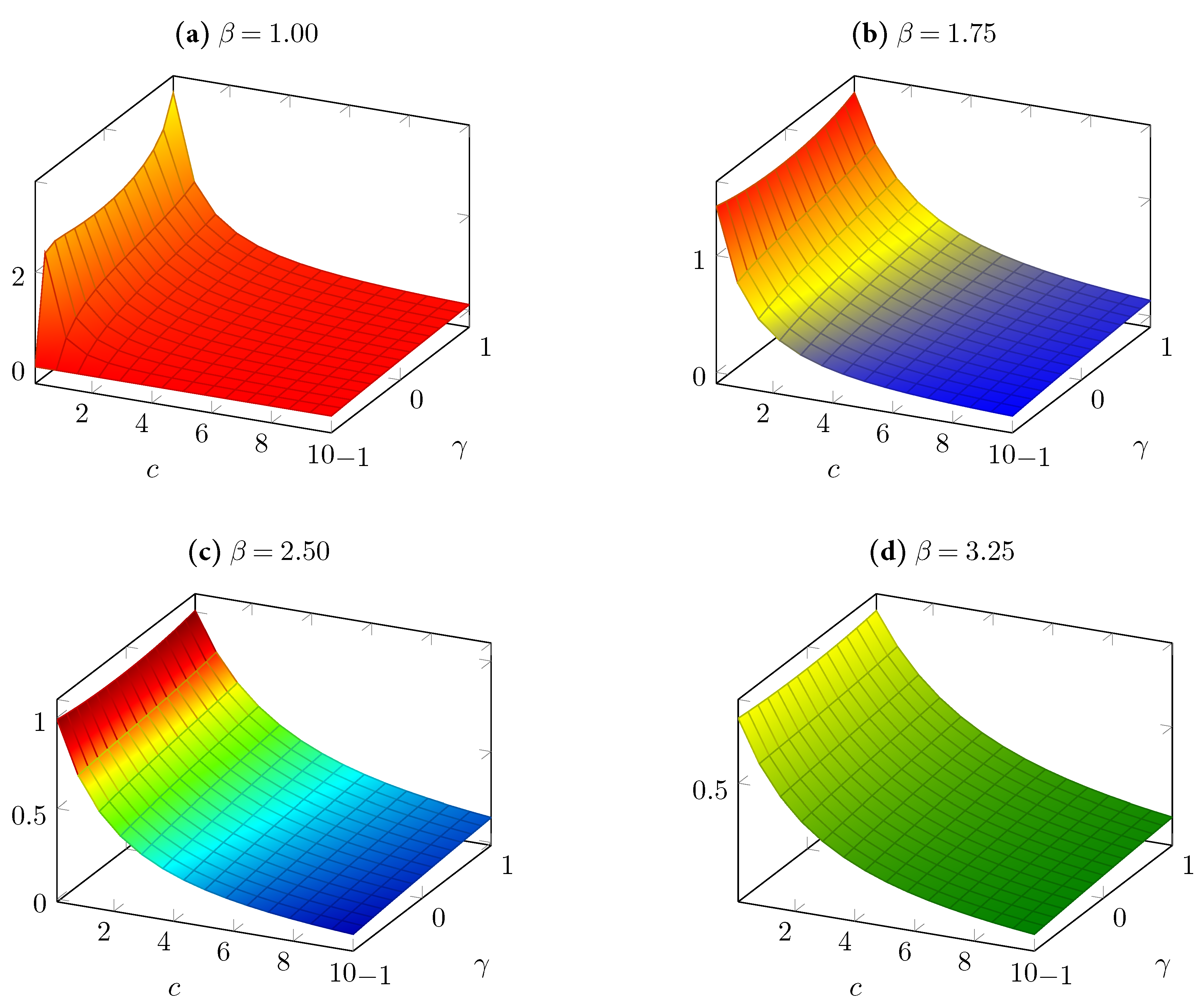
Figure 1 and Figure 2 show that keeping all other parameters constant, the greater the value of the parameter β , the smaller the expected producer profits and the expected consumer surplus.3 Moreover, we found that the cost parameter c had a negative impact on the welfares of both producers and consumers, as theoretically predicted by Corollary 4. On the other hand, the parameter γ had asymmetric effects. Fixing all other parameters to be constant, γ measured the degree of product differentiation, and an increase in γ was found to suggest, especially at low values of c, a decrease in the expected producer profits (as shown in Figure 1) and an increase the expected consumer surplus (as shown in Figure 2).
Figure 1 and Figure 2 together suggest that the parameter γ negatively affects the welfare difference E [ π S F ( α ) ] E [ C S S F ( α ) ] . We could further investigate whether, for any range of γ , the difference between the expected industry welfare and consumer welfare could always become positive or negative, if we kept the other parameters fixed. Here, we note that Equations (27) and (29) together imply that 2 E [ π S F ( α ) ] E [ C S S F ( α ) ] 0 if and only if
2 ξ c β + γ .
In general, whether the above inequality holds or not depends, in a nontrivial way, on the relative size of γ with respect to the other parameters in the model. However, for two extreme cases, we can easily make some predictions. One of these cases occurs when γ is arbitrarily close to β , that is, the products are (almost) perfect complements; the other case occurs when γ is arbitrarily close to β , that is, the products are (almost) perfect substitutes. First we note that when γ is (arbitrarily) close to β , the variable 1 / ξ in Equation (33) becomes close to 2 β / ( 1 + 1 + 4 β / c ) . Using these values, Equation (37) can be reduced to
4 β c + 1 4 β c + 1 .
We know that the above inequality is always true. This implies that if the degree of product complementarity is sufficiently high, the expected total welfare of the duopolists can become always higher than the expected welfare of the consumers. Now, we consider the opposite case in which γ is (arbitrarily) close to β . Then, the variable 1 / ξ becomes close to 2 β / ( 1 + 1 + 4 β / c ) , as in the previous case. With these values, Equation (37) can now be reduced to
4 β 1 + 1 + 4 β / c c 2 β ,
which can be shown to be satisfied if and only if β / c ( 1 + 2 ) / 2 . Thus, we can conclude that when the degree of product substitution is sufficiently high, the expected total welfare of the duopolists can become higher than the expected welfare of the consumers if and only if the marginal cost of a unit output is sufficiently high.

3.3. Welfare Ranking

Now, we investigate whether the supply function competition or the quantity competition can always yield a higher expected welfare to the duopolists or the consumers in the studied industry.
Proposition 3.
In the studied duopolistic industry with differentiated products and demand uncertainty, the expected consumer surplus under the supply function competition is always higher than under the quantity competition.
Proof. 
Comparing Equations (18) and (29) using Equations (30) and (31), we observe that E [ C S S F ( α ) ] > E [ C S C ( α ) ] if and only if
( β + γ ) ξ 1 + ξ ( β + γ ) 2 1 + η 2 ( E [ α ] ) 2 > ( β + γ ) 1 2 β + γ + c 2 ( E [ α ] ) 2 .
We know that η > 0 (as there is demand uncertainty by assumption). First, we assume the limiting case of η = 0 . Then Equation (40) would be equivalent to ξ > 1 / ( β + c ) , which, from the definition of ξ in Equation (32), is equivalent to γ 2 > 0 . We have | γ | 0 by assumption, implying Equation (40) when η = 0 . Moreover, because the left-hand side of Equation (40) is increasing in η while its right-hand side is independent of it, Equation (40) must hold for all η > 0 . Thus, it is always true that E [ C S S F ( α ) ] > E [ C S C ( α ) ] . ☐
Now, we can consider a welfare comparison from the viewpoint of the producers. First we note that using Equations (30) and (31), the expected producer profits in Equation (27) can be rewritten as
E [ π S F ( α ) ] = 1 ξ c 2 ξ 1 + ξ ( β + γ ) 2 1 + η 2 E [ α ] 2 .
If E [ α ] remains unchanged, the demand uncertainty, measured by η , positively affects the expected profits in Equation (41) obtained by each duopolist under the supply function competition, while it has no effect on the expected profits in Equation (14) that each duopolist obtains under the quantity competition. Thus, the profit difference E [ π S F ( α ) ] E [ π C ( α ) ] is increasing in η when E [ α ] is constant. We let η ¯ be the lowest value of demand uncertainty at which this profit difference is nonnegative, that is, η ¯ : = min { η 0 : E [ π S F ( α ) ] E [ π C ( α ) ] 0 } . This value can be calculated using Equations (14) and (41) as follows:
η ¯ = max 0 , 1 + β + c 2 1 ξ + β + γ 2 1 ξ c 2 2 β + γ + c 2 .
We note that the coefficient of variation η is always nonnegative, and when it is above (below) the critical level η ¯ , the expected producer profits under the supply function competition are higher (lower) than those under the quantity competition.
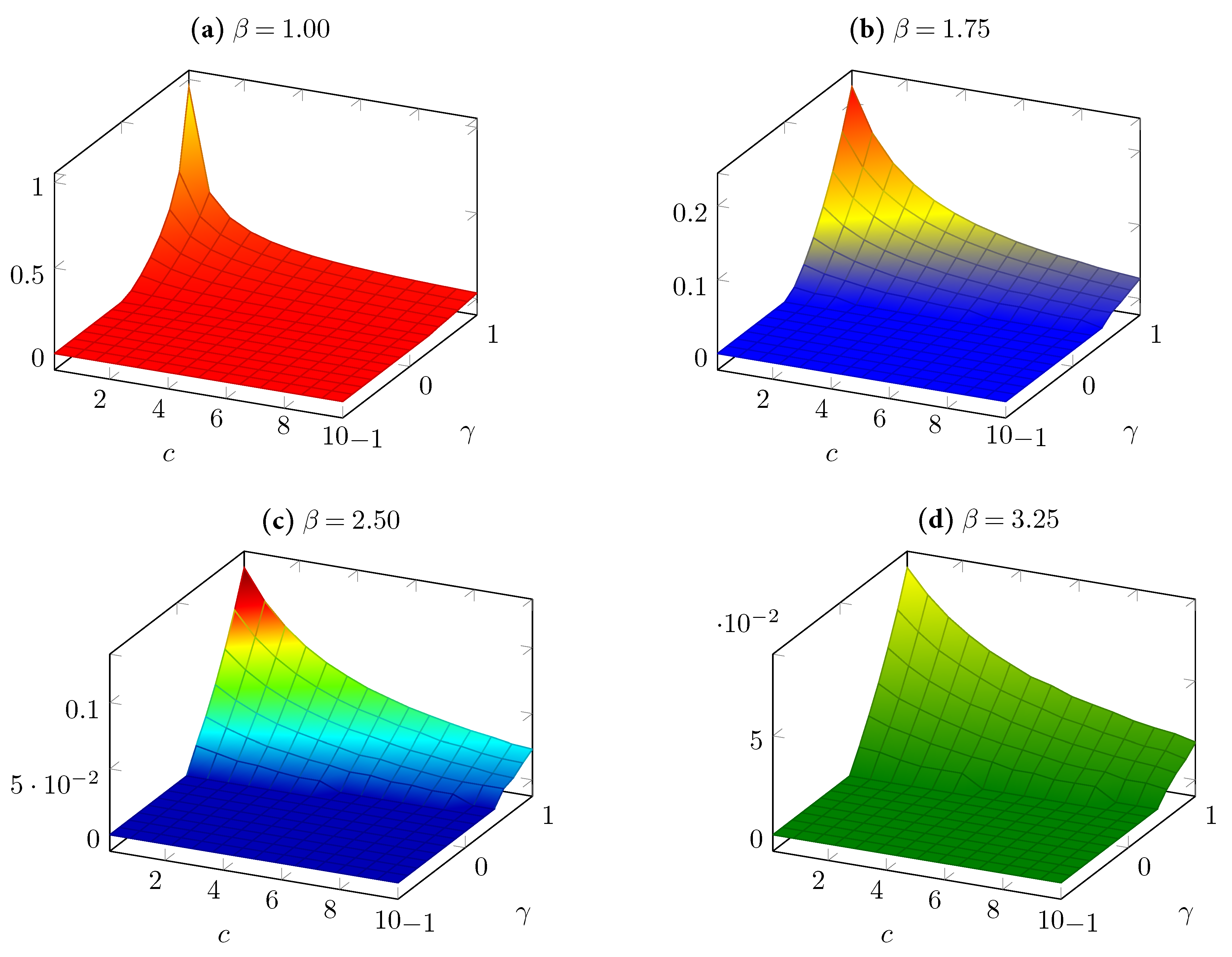
Now, we investigate how the critical level of demand uncertainty, η ¯ , is affected by a change in any of the parameters β , γ , or c. However, because of the complexity of Equations (32) and (42), we were able to do this only by numerical simulations. We plot in Figure 3 the simulated graphs of η ¯ . (The ranges of β , γ , and c are as in the previous two figures). Comparing all four graphs in Figure 3 reveals that for extremely low values of γ , the value of η ¯ becomes almost zero, implying that at such values of γ , the expected producer profits are almost always higher under the supply function competition than under the quantity competition.
Figure 3 also suggests that η ¯ is always positive, implying that for sufficiently low values of demand uncertainty, duopolistic firms prefer the quantity competition to the supply function competition. Another finding from Figure 3 is that an increase in β decreases η ¯ at all values c in its domain when γ is not negative (when the products are neither complements nor independent) and is also not low (when the product substitution is high). This implies that if, for each product, the demand becomes smaller as a result of an increase in its own-price sensitivity, then the supply function competition would require a lower amount of uncertainty to dominate the quantity competition from the viewpoint of the duopolists. A similar result is also observed when the marginal cost of producing a unit output, c, becomes higher. On the other hand, the differentiation parameter γ , when it is positive and sufficiently high, has a positive effect on η ¯ . That is, as the products in the industry become closer substitutes, then the supply function competition would, in general, require a higher amount of uncertainty to dominate the quantity competition from the viewpoint of the duopolists.

4. Conclusions

In this paper, we make a welfare comparison between the supply function and quantity competitions in a duopolistic industry with differentiated products and demand uncertainty. We present in Propositions 1 and 2 the characterizations of the symmetric equilibrium obtained under each form of competition, and by calculating the expected welfares of the producers and consumers at each of these equilibria, we first study how they would respond to changes in various model parameters. These parameters are the size of the demand uncertainty measured by the coefficient of variation ( η ) when the expected demand uncertainty E [ α ] is fixed; the own-price sensitivity of the demand curves measured by the parameter β when γ is fixed; the degree of product differentiation measured by the parameter γ when β is fixed; and the marginal cost, to produce a unit output, measured by the parameter c.
Under the quantity competition, both the expected consumer surplus and the expected producer profits are independent of η , while both of them are always decreasing in c. On the other hand, the parameters β and γ can have asymmetric effects on the welfares of the duopolists and the consumers. Whereas the expected profits of the duopolists are always decreasing in β and γ , the expected consumer surplus can be increasing in these two parameters unless the marginal cost of producing a unit output is sufficiently small for each duopolist. Under the supply function competition, we find that both the expected consumer surplus and the expected profits of the duopolists are always increasing in the size of demand uncertainty, η , while they are always decreasing in the marginal cost c of a unit output. Additionally, our numerical simulations suggested that the welfares of both producers and consumers always decrease the sensitivity parameter β of the inverse demand to the own output. On the other hand, the product differentiation parameter γ has different effects on the expected welfares of producers and consumers. An increase in γ is found to decrease the expected producer profits while increasing the expected consumer surplus.
Next, we study how moving from one type of competition to the other can affect the expected welfares of producers and consumers. In Proposition 3, we show that the expected consumer surplus under the supply function competition is always higher than that under the quantity competition. By some numerical simulations, we also observed that the expected producer profits under the supply function competition can be lower than those under the quantity competition if and only if the parameter of the product differentiation ( γ ) is nonpositive or is sufficiently small and the size of the demand uncertainty ( η ) is below a critical level ( η ¯ ) that is nonincreasing in c and β and nondecreasing in γ .
The main results of this paper are that, in a differentiated products duopoly with demand uncertainty, (i) if the products are either complements or independent, or if they have an extremely low degree of substitution, then the supply function competition can always be Pareto superior to the quantity competition, and (ii) if the degree of product substitution is not extremely low, then the supply function competition can be Pareto superior to the quantity competition if and only if the size of the demand uncertainty is sufficiently large. The second of these results is an extension of an earlier result of Saglam (2018) [11] obtained for a homogeneous product duopoly. Overall, our results suggest that in electricity markets with differentiated products, the regulators should not intervene to impose the quantity competition in favor of the supply function competition unless the degree of product substitution is sufficiently high and the predicted demand fluctuations are sufficiently small.

Funding

This research received no external funding.

Acknowledgments

The author thanks two anonymous reviewers for many comments and suggestions that substantially improved this paper. The usual disclaimer applies.

Conflicts of Interest

The author declares no conflict of interest.

References

  1. Grossman, S. Nash equilibrium and the industrial organization of markets with large fixed costs. Econometrica 1981, 49, 1149–1172. [Google Scholar] [CrossRef]
  2. Klemperer, P.D.; Meyer, M.A. Supply function equilibria in oligopoly under uncertainty. Econometrica 1989, 57, 1243–1277. [Google Scholar] [CrossRef]
  3. Bertrand, J. Review of théorie mathématique de la richesse sociale and of recherches sur les principles mathématiques de la theorie des richesses. J. Savants 1883, 67, 499–508. [Google Scholar]
  4. Cournot, A.A. Recherches sur les Principes Mathematiques de la Théorie des Richesses; Hachette: Paris, France, 1838. [Google Scholar]
  5. Green, R.J.; Newbery, D.M. Competition in the British electric spot market. J. Polit. Econ. 1992, 100, 929–953. [Google Scholar] [CrossRef]
  6. Rudkevich, A.; Duckworth, M. Strategic bidding in a deregulated generation market: Implications for electricity prices, asset valuation and regulatory response. Electr. J. 1998, 11, 73–83. [Google Scholar] [CrossRef]
  7. Rudkevich, A.; Duckworth, M.; Rosen, R. Modeling electricity pricing in a deregulated generation industry: The potential for oligopoly pricing in a poolco. Energy J. 1998, 19, 19–48. [Google Scholar] [CrossRef]
  8. Delbono, F.; Lambertini, L. Ranking Bertrand, Cournot and supply function equilibria in oligopoly. Energy Econom. 2016, 60, 73–78. [Google Scholar] [CrossRef] [Green Version]
  9. Monden, A. Worst Welfare under the supply function competition with sequential contracting in a vertical relationship. J. Game Theory 2017, 6, 38–42. [Google Scholar]
  10. Ciarreta, A.; Gutiérrez-Hita, C. Supply function vs. quantity competition in supergames. Int. J. Ind. Organ. 2006, 24, 773–783. [Google Scholar] [CrossRef]
  11. Saglam, I. The desirability of the supply function competition under demand uncertainty. Econom. Bull. 2018, 38, 541–549. [Google Scholar]
  12. Woo, C.K.; Sreedharan, P.; Hargreaves, J.; Kahrl, F.; Wang, J.; Horowitz, I. A review of electricity product differentiation. Appl. Energy 2014, 114, 262–272. [Google Scholar] [CrossRef]
  13. Singh, N.; Vives, X. Price and quantity competition in a differentiated duopoly. RAND J. Econom. 1984, 15, 546–554. [Google Scholar] [CrossRef]
  14. Nash, J. Equilibrium points in n-person games. Proc. Natl. Acad. Sci. USA 1950, 36, 48–49. [Google Scholar] [CrossRef] [PubMed] [Green Version]
1.
Woo et al. (2014) [12] support their argument by pointing to several distinct attributes of electricity—such as quality, reliability, time of use, consumption volume, maximum demand, and environmental impact—that can be packaged at alternative proportions.
2.
Singh and Vives (1984) [13] study the effects of the degree of product differentiation on the duopolistic firms’ choices between the price and quantity contracts with consumers.
3.
We also found that the effects of β , as shown in Figure 1 and Figure 2, remained unchanged when we increased β to some higher levels outside its simulation range.
Figure 1. Plots of E [ π S F ( α ) ] for various values of β , γ , and c when E [ α 2 ] = 10 .
Games 09 00060 g001
Figure 2. Plots of E [ C S S F ( α ) ] for various values of β , γ , and c when E [ α 2 ] = 10 .
Games 09 00060 g002
Figure 3. Plots of η ¯ for various values of β , γ , and c.
Games 09 00060 g003

