Game Theoretical Model of Cancer Dynamics with Four Cell Phenotypes

Abstract

The development of a cancerous tumor requires affected cells to collectively display an assortment of characteristic behaviors that contribute differently to its growth. A heterogeneous population of tumor cells is far more resistant to treatment than a homogeneous one as different cell types respond dissimilarly to treatments; yet, these cell types are also in competition with one another. This paper models heterogeneous cancer cell interactions within the tumor mass through several game theoretic approaches including classical normal form games, replicator dynamics, and spatial games. Our concept model community consists of four cell strategies: an angiogenesis-factor-producing cell, a proliferative cell, a cytotoxin producing cell, and a neutral stromal cell. By comparing pairwise strategic interactions, invasibility and counter-invasibility, we establish conditions for dominance and the existence of both monomorphic and polymorphic equilibria. The spatial game supports co-occurrence among multiple subpopulations in accordance with biological observations of developing tumors. As the tumor progresses from primarily stromal cells to a more malignant state, angiogenic and cytotoxic cells form clusters while proliferative cells are widespread. The clustering of certain subpopulations suggests insight into the behaviors of cancer cells that could influence future treatment strategies.

1. Introduction

Cancer is a disease in which abnormal cells uncontrollably proliferate, thereby disrupting the homeostatic state of a given tissue, and, in their most malignant form, disperse to other parts of the host body [1]. The transformation of healthy cells into a cancerous mass is driven by somatic evolution favoring those cells that have been able to ignore, at least partially, the normal regulatory controls on replication [2,3]. Early thoughts on cancer held that tumors were simply collections of homogeneous cells. Modern understanding recognizes that, rather than being a uniform mass of cells, cancerous tumors are more often a heterogeneous population of cells expressing multiple phenotypes [4,5,6,7], both among tumor cells and also the host stromal cells [8,9]. This heterogeneity complicates treatment of the tumor as different cell types will respond dissimilarly to treatment protocols [10]. Additionally, although they share a potentially mutualistic association during tumor-host interactions, these cancer cell phentoypes remain in competition with one another for space, nutrients and other cellular resources [2,3,7,10,11,12]. Tumors need to exhibit multiple qualities before the neoplasm advances to a fully malignant cancerous state. Hanahan and Weinberg [13] originally laid out six main characteristics dubbed the hallmarks of cancer [13]. These biological capabilities included self-sufficiency in growth signals, insensitivity to anti-growth signals, evading apoptosis, unlimited replicative potential, sustained angiogenesis, and tissue invasion and metastasis. When the authors revisited their paper a decade later [8], they augmented the previous list with two additional hallmarks—reprogramming of energy metabolism, and evading immune destruction—as well as two enabling conditions—genome instability [14] and inflammation driving by immune system [15]. Pavlova and Thompson recently provided a similar set of six metabolic hallmarks characterizing the metabolic reprogramming [16]. These acquired capabilities have since become the focus of many mathematical models in studying the behavior of cancer cells [17].

Cancer cells exist within a complex tissue microenvironment composed of a heterogeneous collection of stromal and cancer cells, dispersing extracellular components, and structural aspects such as vascularization [1,8,12,18,19,20]. During tumorigenesis cancer cells develop strategies to scavenge nutrients from the extracellular matrix (e.g., glucose or glutamine) or co-opt neighboring stromal cells to provide the resources needed for persistence and tumor growth [16]. This disruption of regulating processes enables survival and proliferation even in resource-poor environments. Tumor cells can take advantage of these tumor-associated stromal cells (TASCs) by manipulating them to express reactive phenotypes more often associated during wound healing [21] or to otherwise engage in metabolic activities [1,22]. TASCs include fibroblasts, pericytes, and adipocytes plus other specialized cells [1,20,22]. Cancer-associated fibroblasts (CAFs) constitute a significant proportion of the actual tumor mass in, for example, breast cancer, pancreatic cancer [20], and prostate cancer [23]. They promote oncogenic development by secreting components into the extracellular matrix which can then be absorbed by cancer cells [9]. Cell types subsequently coevolve in response to direct cell-to-cell interactions and indirect alterations to the surrounding microenvironment [20].

Here we study the evolution of the composition of tumors from three game-theoretic perspectives: classical two-player games, population-level replicator dynamics, and spatially structured games. Our concept model tissue is composed of cells potentially exhibiting four distinct phenotypes: neutral stromal cells, angiogenesis-factor producing cells, cytotoxin-producing cells, and proliferative cells. We explore the potential equilibria that can emerge between malignant cell types and prove that persistent oscillation of cell phenotypes (e.g., a rock-paper-scissors scenario) cannot occur within either a normal-form game or a replicator dynamics system for this toy model. Both discrete time and continuous time interpretations are considered for replicator dynamics. The final component of our study extends the evolutionary game to a spatial framework to observe the effects that spatial structure and parameter variation have on tumor development and its heterogeneity.

The heterogeneity of tumors and the cooperative and competitive behaviors of the phenotypes therein make game theory a highly appropriate perspective from which to evaluate and predict the interactions between the various phenotypes expressed by the constituent cells [24,25]. Classical game theory can assess the best responses to competing phenotypes, while one can estimate the relative prevalence of phenotypes when polymorphic populations occur through evolutionary game theory [26,27]. The frequencies of behavioral phenotypes within the tumor mass change over time in response to their relative fitness, and such fitness measures may be frequency dependent rather than static. Other game theoretical studies have identified which parameter combinations led to different phenotypic fixations or to polymorphisms (reviewed in [28]). Those studies have considered a number of different cell phenotypes that involve proliferation [2], angiogenesis or paracrine/autocrine secretions [29], motility [2,30], cytotoxicity and local acidosis [31,32], glycolosis [2], avoidance of apoptosis [29], metabolic respiration, proliferation [2] and other cancer-specific properties. The studies have also addressed a wide range of types of cancer such as glioma progression [2,10,33], colorectal carcinogenesis [34], multiple myeloma [35], and prostate cancer [10].

A major development in recent game theory has been the imposition of spatial structure on top of traditional games. Early studies have explored the development and maintenance of cooperation in the prisoner’s dilemma as well as other models [36,37]. Spatial games are particularly relevant to the study of cancer growth as cell reproduction and resource competition is localized during tumorigenesis [12]. To add this level of biological realism, Bach et. al. [38] reconsidered Tomlinson and Bodmer’s [29] original angiogenesis game using a spatial frequency-dependent model. The spatial model yielded results that differed from the mean-field simulations but showed that cooperative promoter strategies are frequently out-competed by non-promoters [38]. An elaboration of this study used a mixed strategy game and supplemented an additional strategy for cells that produce growth factors [39]. Alternatively, cell automaton models have been adopted to explore the effects of space and allowing occupation by one or more cells at each site on the lattice where resources will be shared [2]. The mechanisms for updating the system for reproduction and mortality and resource control are varied but more closely represent intratumor interactions.

Our approach to identifying Nash equilibria among pure strategies follows the standard procedure of comparing the payoffs of alternate strategies to assess the best response to each phenotype. Likewise our replicator equations will assume that fitness levels are calculated via mean-field averages [40]. The implementation of the spatial game in our model parallels the two-phenotype model of Bach [38] with a random selection of cells replaced by other cells within a local neighborhood. We differ in how the two demographic processes within our simulation are implemented with respect to the model’s parameter values.

While all phenotypes are present in at least some strategic solutions, as determined by parameter combinations, angiogenesis-factor producing and proliferative cells are the most frequently occurring cell types within the model tumor in all three treatments. Moreover, as the tumor progresses from primarily stromal cells to a more malignant state, our spatial simulations suggest that angiogenic and cytotoxic cells form clusters, while proliferative cells have a more widespread encroachment of stromal cell tissue. Clustering may emerge even when parameters contra-indicate the elimination of these phenotypes in the classical game or under replication dynamics. This phenotypic patterning offers a potential insight into the targeted treatments for specific cancer cell types.

The organization of this paper is as follows. Section 2 develops a traditional normal-form, symmetric matrix game and identifies the conditions in which different Nash equilibria emerge among pure strategy players. Section 3 translates the static game into an evolutionarily dynamic game of changing population frequencies under replicator dynamics. Finally, we introduce a spatial game variant in Section 4 in which the payoff components affect either a cell’s propensity to expire or to populate an adjacent vacancy. We conclude with our observations of the different modeling approaches.

2. Classical Game Theory

Our research considers the interplay of four distinct cell phenotypes that might be present within a cancer tumor. Stromal cancer cells (A−) have no particular benefit or cost unique to themselves, and they are considered a baseline neutral cell within the context of the model. In constrast, angiogenesis-factor producing cells (A+) vascularize the local tumor area which consequently introduces a nutrient rich blood to the benefit of all interacting cells. Nutrient recruitment expands when A+ cells interact with one another. Cytotoxic cells (C) release a chemical compound which harms heterospecific cells and increases their rate of cell death. The cytotoxic cells benefit from the resulting disruption in competition caused by the interaction. For simplicity, our model presumes that cytotoxic cells are themselves immune to this class of agent. Finally, proliferative cells (P) possess a reproductive or metabolic advantage relative to the other cell types. In our model this advantage does not compound with the nutrient enrichment produced by vascularization when A+ cells are present; however, it does place the proliferative cell at a greater vulnerability to cytotoxins.

Table 1. Parameters used within the game and dynamic models.

Parameter	Interpretation
a	Cost of producing angiogenesis factors
b	Cost of producing cytotoxin
c	Cost of interaction with cytotoxin
d	Resource benefit when interacting with A+
e	Exploitation benefit for C when cytotoxin damages others
f	Synergistic resource benefit when two A+ cells interact
g	Reproductive advantage of P cell

gives an overview of all parameters involved in our study reflecting this description.

Our first treatment considers a classical symmetric game between two players. Each player, representing a cell within the tissue, can adopt one of the four phenotypic strategies described above, and they receive payoffs in accordance with

Table 2. Payoff matrix of four cancer cell phenotypes.

Player\Opponent	A−	A+	P	C
A−	1	$1+d$	1	$1-c$
A+	$1-a+d$	$1-a+d+f$	$1-a+d$	$1-c-a+d$
P	$1+g$	$1+d+g$	$1+g$	$(1+g)(1-c)$
C	$1-b+e$	$1-b+d+e$	$1-b+e$	$1-b$

. Our goal is to identify all pure strategy Nash equilibria that are possible and in what parameter regions the game permits a cyclic best response phenomenon (i.e., a rock-paper-scissors scenario). As part of our analyses, we consider not only games in which all four strategies are available but also those reduced games where some strategies are specifically excluded.

The diagonals of this payoff matrix represent interactions within monomorphic populations while the off-diagonal elements represent fitness values when the cells are in a polymorphic state. A self-similar Nash equilibrium corresponds to a monomorphic population where the dominant phenotype is its own best response. A stable polymorphism is then any other Nash equilibrium solution to the game.

Now consider first those games in which there are only two options for the phenotype strategy (

Table 3. Pairwise contrast of strategies. Each pair of strategies is compared in a reduced two-strategy game, with the stated outcome given by the listed condition(s). If there are additional conditions that arise for strict dominance when all four strategies are available, these are listed under “Greater Context”.

Contrast	Outcome	Condition	Greater Context
A+ vs. A−	A+ dominates	f, $d>a$	None
	A− dominates	f, $d<a$	None
	Exclusion	$d<a<f$	–
	Sympatry	$f<a<d$	–
A+ vs. P	A+ dominates	f, $d>a+g$	None
	P dominates	f, $d<a+g$	$d<a+g(1-c)$
	Exclusion	$d<a+g<f$	–
	Sympatry	$f<a+g<d$	–
A+ vs. C	A+ dominates	$f>a+(e-b)$, $d>a+(c-b)$	$d>a+(e-b)$
	C dominates	$f<a+(e-b)$, $d<a+(c-b)$	$d<a+(e-b)$
	Exclusion	$f>a+(e-b)$, $d<a+(c-b)$	–
	Sympatry	$f<a+(e-b)$, $d>a+(c-b)$	–
A− vs. P	A− dominates	$g<0$	$c<1$
	P dominates	$g>0$	$c<1$
	Exclusion	N/A	–
	Sympatry	$g=0$	–
A− vs. C	A− dominates	$b>c$, e	None
	C dominates	$b<c$, e	None
	Exclusion	$e<b<c$	–
	Sympatry	$c<b<e$	–
P vs. C	P dominates	$b+g>c(1+g)$, e	None
	C dominates	$b+g<c(1+g)$, e	None
	Exclusion	$e<b+g<c(1+g)$	–
	Sympatry	$c(1+g)<b+g<e$	–

). Each pair of strategies is compared within the restricted game for dominance, mutual exclusion, or mutual best response. Pairwise strict dominance is achieved when the dominant strategy is the best response both to itself and to the alternative strategy, and this Nash equilibrium corresponds to a strategically stable monomorphic population. Sympatry or coexistence is achieved when the two alternative strategies are the best responses to each other, producing a stable polymorphism. Finally, if each strategy is its own best response, the population has two possible monomorphic states (bistability).

Table 3 also lists any additional conditions, if any, that are necessary to impose strict dominance between the strategies in the broader context of the full four-strategy game.

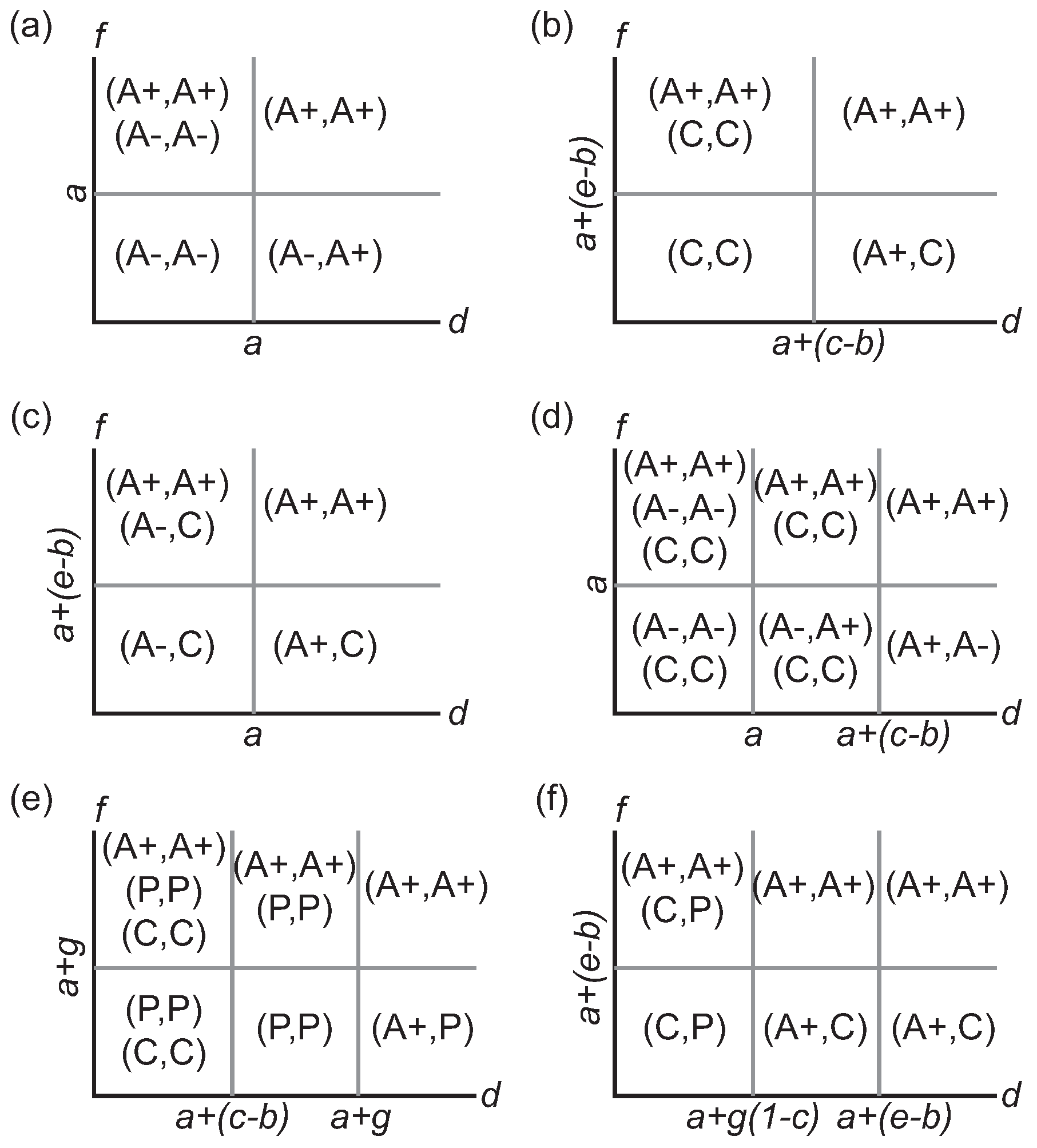
For every pair of competing strategies, there is a clear partition of the parameter space in which dominance, exclusion, or mutual best response characteristically occur Figure 1a,b gives the representative quadrants within the $(d,f)$ parameter space where these outcomes occur.

In a game played among the three non-proliferative cell types, each cell phenotype emerges as part of a Nash equilibrium for some parameter combination (Figure 1a–d). A primary consideration in assessing parameter regions is the relative ordering of the three parameters pertaining to the use of cytotoxin (b, c, e). The other main determinant is how extensive the basic and synergistic benefits of growth-factor production are.

The phenotype game and its restricted forms demonstrate a wide variety of strategic outcomes (Figure 1). Mutual exclusion, where strategies are their own best response, is prominent when the basic benefits of vascularization are small (e.g., $d<a$) but the synergistic effects are high (e.g., $f>a+g$, Table 3). When the reverse holds, with high benefits but low synergy, polymorphic solutions are typically formed between A+ and a non-angiogenic cell.

Stromal cells are part of Nash equilibria only under limited circumstances in the full game. When the proliferative phenotype—which is the primary factor in their exclusion—is introduced as a strategy within the game, it strictly dominates the stromal cell whenever the cost of exposure to cytotoxins is small ($c<1$). Consequently, its inclusion effectively reduces the full phenotypic game to a three-strategy game involving only the non-stromal cells. As we observed in the previous restricted game, specific parameter regions support different Nash equilibria (Figure 1e,f). The main difference is that the primary partitioning of the parameter regions is based upon the ordering of the parametric combinations g, $(e-b)$, and $(c-b)/(1-c)$ rather than the cytotoxic parameters b, c, and e. Proliferative cells enjoy a broad advantage appearing in a majority of the Nash equilibria, particularly in the symmetric response solution $(\mathrm{P},\mathrm{P})$; however, the set of equilibria across all parameters does include all six possible pure-strategy combinations (up to symmetry).

A final conclusion of our analysis is that an oscillatory strategem such as rock-paper-scissors does not emerge in the phenotype game. For each possible triplet, internal contradictions arise that prevent the advent of cyclic dynamics.

Theorem 1.

The matrix game shown in Table 2 does not contain a three-strategy best-response cycle among its available strategies.

The proof of this result can be found in Appendix A.

3. Replicator Dynamics

Under replicator dynamics [40], the frequencies of different strategies or behaviors evolve to favor those strategies whose fitness is greater than the average fitness within the population. The evolution may occur over discrete generational time or on a continual basis. In this interpretation, the variables $u_i$ ($i=1$ to 4) represent the frequencies of stromal, angiogenic, proliferative, and cytotoxic cells within the tissue, respectively. Taking G to be a $4\times 4$ matrix containing the payoff values in Table 2, each phenotype has a corresponding fitness $f_i$ that depends upon the composition of the overall population,

$$\mathbf{f}=G\mathbf{u}.$$

(1)

Here $\mathbf{f}$ and $\mathbf{u}$ are vectors containing the four fitnesses and frequencies, respectively. If the average fitness within the population is equal to the weighted sum

$$f_{\mathrm{avg}}=\sum _{i=1}^4{f}_i{u}_i,$$

(2)

then for discrete time replicator dynamics, the generational update equation is

$$u_i(t+1)=\frac{f_i(\mathbf{u})}{f_{\mathrm{avg}}}{u}_i(t).$$

(3)

The relative fitness of two phenotypes is equal to the ratio of their reproductive fitness measures. In continuous time, however, the rate of change in phenotypic frequency is proportional to both the strength of selection (now the difference in phenotypic fitness) as well as the relative likelihood of encounter between the two phenotypes (the variance within the population). This yields the replicator equation

$$\begin{array}{cc}\hfill \frac{d{u}_i}{dt}& =\sum _{j=1}^4\left(f_i(\mathbf{u})-f_j(\mathbf{u})\right)u_i{u}_j\hfill \\ & =u_i\left(f_i(\mathbf{u})-f_{\mathrm{avg}}\right).\hfill \end{array}$$

(4)

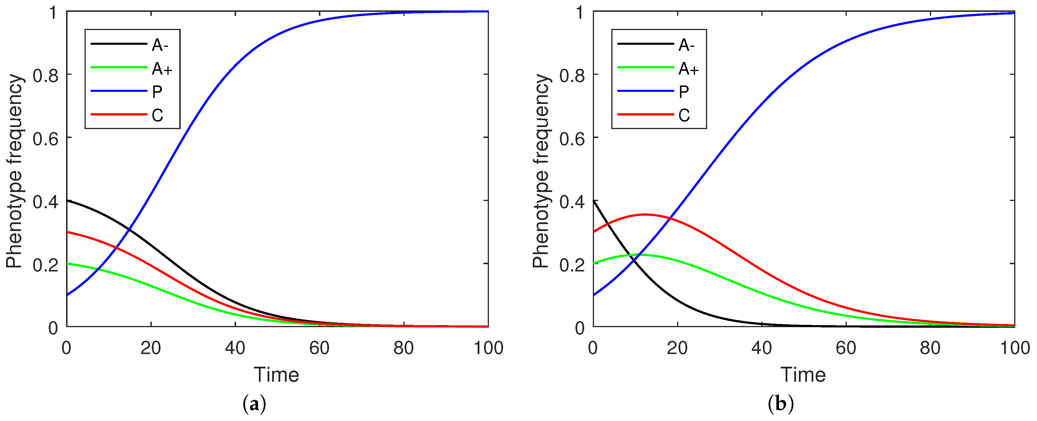
The discrete and continuous replicator dynamics are similar if not identical in their details and predictions, e.g., in the admissibility of negative fitness values. Figure 2 illustrates sample frequency evolutions under both discrete and continuous time.

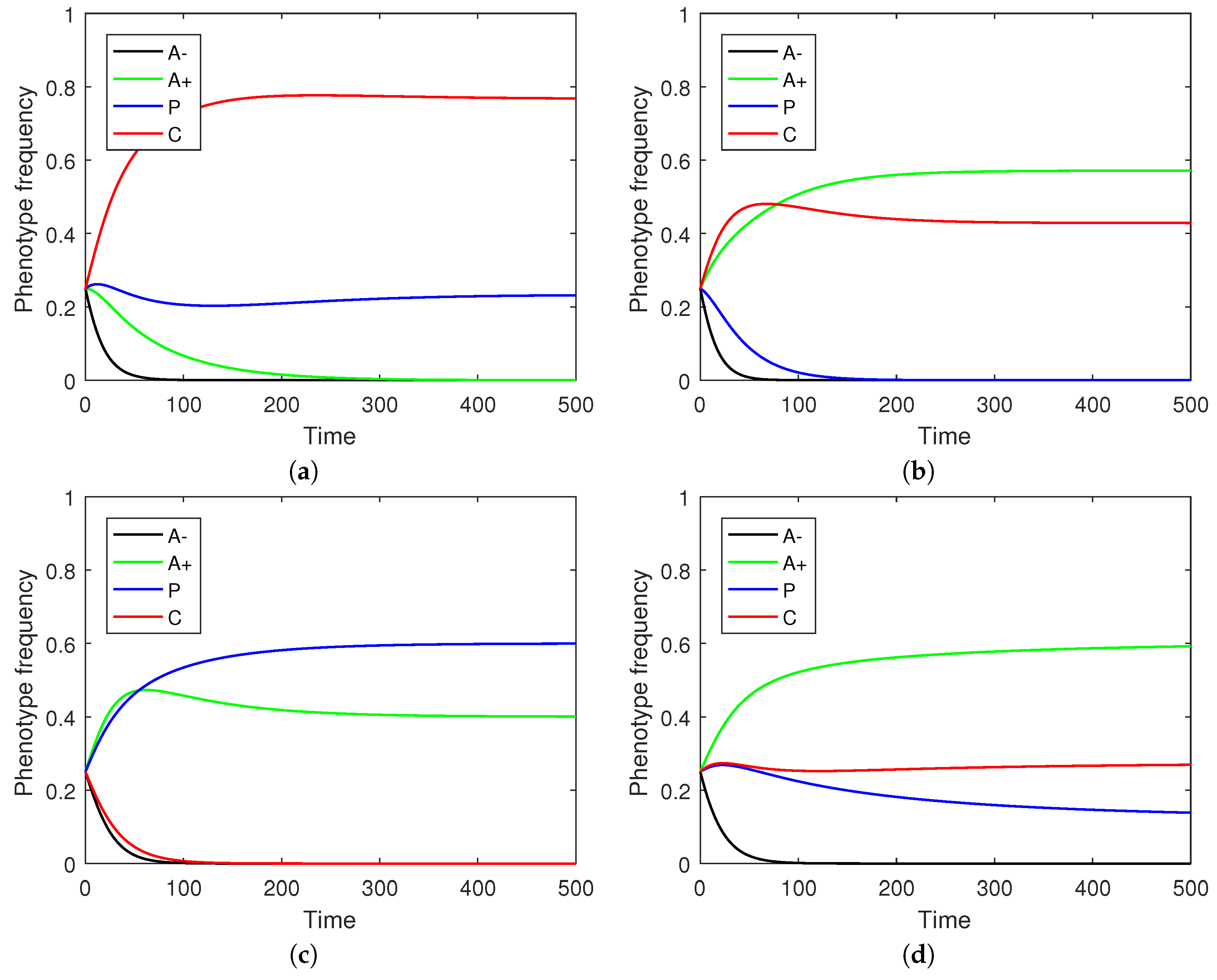
Focusing on the continuous replicator dynamics, each of the non-stromal cells emerge as part of an equilibrium under appropriate parametric constraints both pairwise and in systems where all phenotypes are included together (Figure 3). This parallels the maintenance of different Nash equilibria in the strategic game. The evolution of a phenotype’s evolution need not be monotone (Figure 2) but rather reflect a transitional shift in prevalences through successive dominant phenotypes (e.g., the transition from A− to C and then to P in Figure 2b).

To compute the possible polymorphic equilibrium states of the replicator equations, one simply constructs a new system of equations to represent the constraints $f_h-f_k=0$ for all indices h and k of persistent phenotypes, plus the frequency constraint ${\sum }_k{u}_k=1$. The system is linear in the $u_k$ terms, and there is at most one non-trivial equilibrium ${\mathbf{u}}^{*}$. Thus a solution consisting only of non-stromal phenotypes would be determined by

$$\left[\begin{array}{cccc}1& 0& 0& 0\\ d-a-g& f-a-g& d-a-g& d-a-g(1-c)\\ d+b-a-e& f+b-a-e& d+b-a-e& d+b-a-c\\ 0& 1& 1& 1\end{array}\right]{\mathbf{u}}^{*}=\left[\begin{array}{c}0\\ 0\\ 0\\ 1\end{array}\right].$$

(5)

The Jacobian matrix for the stability analysis is provided by

$$J_{ij}=\left[u_i^{*}\left(G_{ij}-\sum _{k=1}^4\left(G_{kj}+G_{jk}\right)u_k^{*}\right)\right].$$

(6)

Ordinarily one expects greater dynamic diversity when all four phenotypes are simultaneously included; however if the cost of exposure to cytoxins is small ($c<1$), then the strict dominance of proliferative cells over A− stromal cells precludes that possibility. That said, it is conceivable for stromal cells to persist in a three-phenotype equilibrium with angiogenic and cytotoxic cells when (1) $c>1$, (2) $u_2^{*}=1/[1-\frac{f-a}{d-a}]$, $u_3^{*}=1/[1-\frac{c-b}{e-b}]$ and $u_1^{*}=1-u_2^{*}-u_3^{*}>0$, and (3) $c{u}_3^{*}>1$. The first condition prevents strict dominance. The second condition is the non-proliferative equilibrium. The final condition limits invasion by proliferative cells.

More generally, If $u_3^{*}$ is the cytotoxic equilibrium frequency in an (A−, A+, C) polymorphism, and $u_3^{**}$ is the frequency in an (A+, C, P) polymporphism, then A− can invade the latter if $c{u}_3^{**}>1$. Thus, the stromal cell can overcome its disadvantage relative to proliferative cells by using a combination of cytotoxic and angiogenic cells to downgrade its rival’s phenotypic fitness with the former while persisting via improved nutrients provided by the latter.

4. Spatial Model

In our final treatment, we created a spatially explicit version of the game with four cell phenotypes. In this multiplayer game, cells reside in a $100\times 100$ lattice with periodic boundaries. Each cell interacts simultaneously with its eight nearest neighbors corresponding to a Moore neighborhood with radius 1 (cf. [41]). During the initialization of the lattice, the tissue is presumed to be composed entirely of cells using the A− strategy. Subsequently 5% of the cells are randomly chosen and assigned one of the remaining three strategies (A+, P, or C). This system state corresponds to a neoplasm that has not yet reached malignancy [42]. Each cell is then characterized by its propensities to suffer cell death and to undergo reproduction when possible. We then perform a series of 1 million asynchronous updates of the lattice according to the following algorithm:

• a cell is chosen to be replaced by one of its neighbors weighted by the mortality propensity; then
• one neighboring cell is chosen to replace the removed cell weighted by the reproduction propensity.

The parameters previously described in Table 1 influence each cell’s propensities. The baseline mortality propensity of each cell phenotype is assumed to be equal to 1. For A− and A+ cells, the mortality propensity increases by c for each cytotoxic C neighbor, while the mortality propensity increases by $c(1+g)$ for proliferative P cells. The latter rule accounts for the additional absorption and, therefore, additional damage from cytotoxin vulnerability as a result of their reproductive advantage g. The baseline reproduction propensity is equal to 1 for A− cells, $1-a+d$ for A+ cells, $1+g$ for P cells, and $1-b$ for C cells. The reproduction propensity of A−, P, and C cells increases by d if they have at least one A+ neighbor, whereas the reproduction propensity of A+ cells cumulatively increases by f for each A+ neighbor due to synergistic effects. Additionally, C cells increase their reproduction propensity by e for each non-cytotoxic neighboring cell to reflect exploitation of weakened competitors. The mortality and reproduction propensities of each of the four cell phenotypes in the spatial game are summarized in

Table 4. Mortality and reproduction propensities in the spatial multiplayer game. Notation: T is the number of C neighbors, A is the number of A+ neighbors.

Phenotype	Mortality Propensity	Reproduction Propensity with No A+ Neighbors	Reproduction Propensity with at Least One A+ Neighbor
A−	$1+Tc$	1	$1+d$
A+	$1+Tc$	$1-a+d$	$1-a+d+Af$
P	$1+Tc(1+g)$	$1+g$	$1+g+d$
C	1	$1-b+(8-T)e$	$1-b+(8-T)e+d$

.

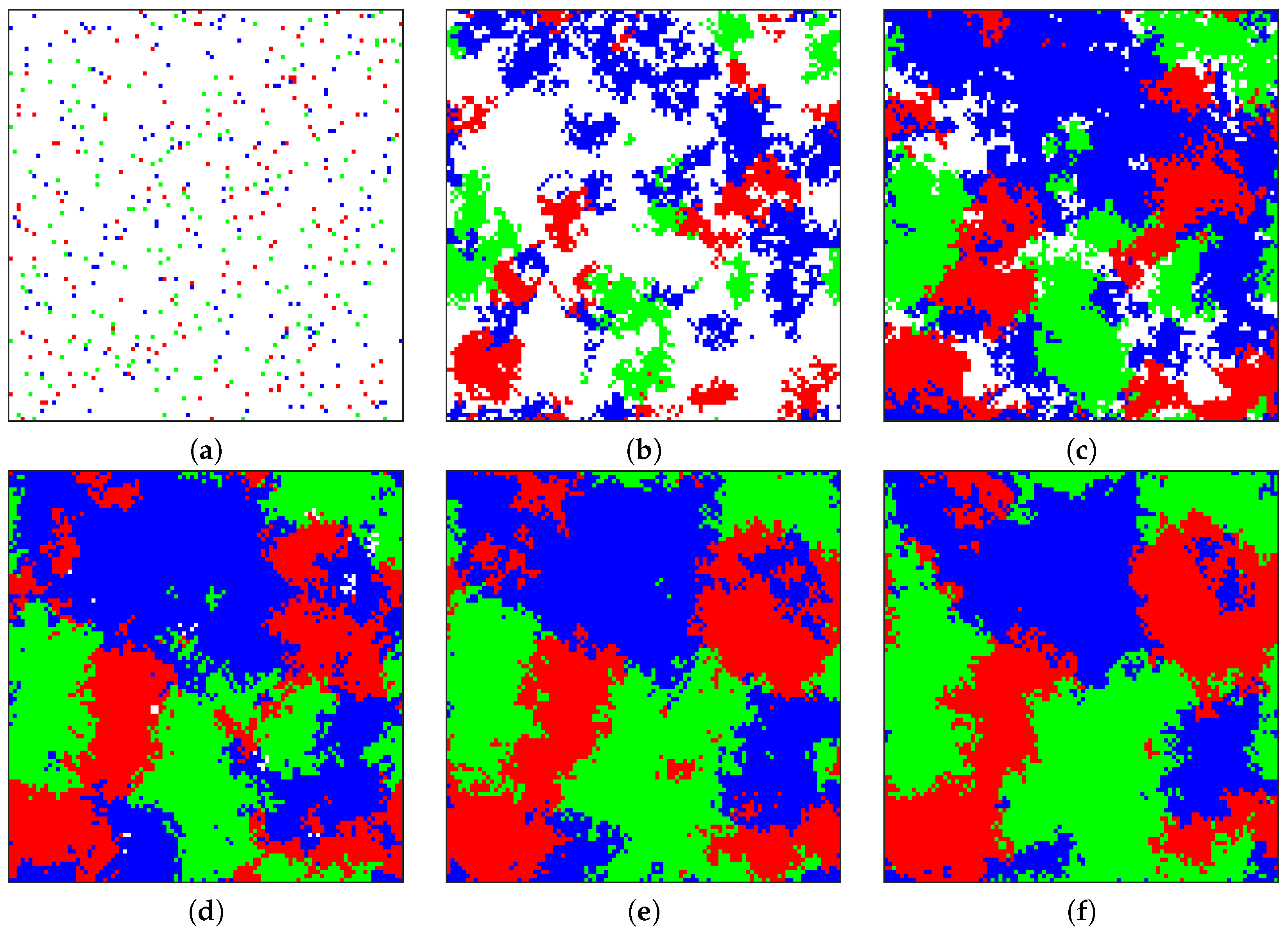
We ran 10,000 trials of the spatial game simulation for each combination of parameters and averaged the results. Figure 4 shows six snapshots of the sample evolution of the tumor from its initial composition to a stage where three cell phenotypes (angiogenic, proliferative, and cytotoxic) exist in roughly equal proportions. The three-way equilibrium is achieved with the following combination of parameters: $a=b=c=d=f=0.1$, $e=0.01$, $g=0.3$. This combination is notable in that these parameters do not correspond to a polymorphic solution for the replicator equations (P strictly dominates all other strategies). Because the game is no longer played by just two individuals but several within a neighborhood, diffusive particles (e.g., growth factors or cytotoxins) can accumulate and have a magnified effect on the game. An accompanying animation video of the progression of the tumor in Figure 4 may be found in the Supplementary Materials.

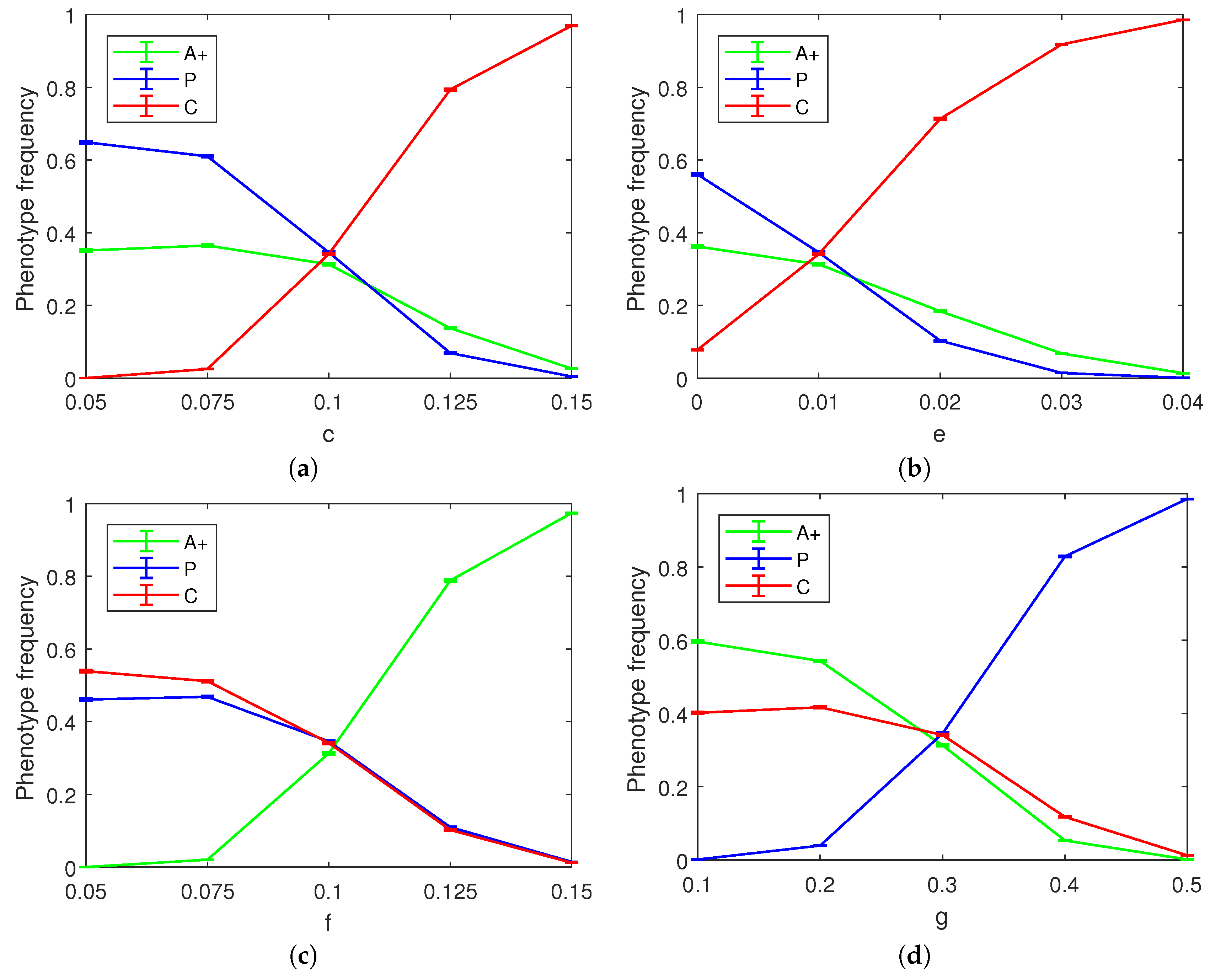
As part of our simulations, we also investigated how each of the parameters c, d, e, f, and g affects the final state of the tumor. We kept all parameters but the focal one fixed at the values corresponding to the three-way co-occurrence mentioned above. As the benefit from simple angiogenesis is agnostic to the recipient cell phenotype, the d parameter did not have a significant effect on the outcome of the spatial game save for a small albeit noticeable reduction in the equilibrium frequency of the P cells as the value of d is increased (not pictured). We surmise that this happens because the baseline reproduction advantage of P cells was relatively less important with larger values of d. Figure 5 shows the effect of varying the four remaining parameters of the spatial model on the final phenotype frequency distribution. As documented in the figure panels, these parameter variations can push the tumor towards a less heterogeneous state dominated by two or even a single phenotype.

5. Discussion

The ability to understand tumor cell interactions may provide an insight to cancer treatment and allow for a more refined process when deciding how to combat tumor growth and development [43,44]; however, predictive and diagnostic capabilities must be preceded first by conceptual models such as ours. We implemented multiple game theoretic perspectives to consider intra-tumor cellular interactions and their effects on the persistence of four distinct phenotypes. The classical game theory approach demonstrated that each of the non-stromal cell phenotypes could persist with or dominate all other strategies whether in pairwise competition or in games where all four phenotypes are available strategies. Although parameters may indicate the persistence of three distinct morphs (most likely the three non-stromal phenotypes), there is no cycling of dominance among them. Dynamical constraints in our model eliminate the possibility of this behavior. The introduction of a spatial lattice to model yielded results very different from the those predicted by classical or replicator games.

Tomlinson and Bodmer [29] applied evolutionary game theory to interactions between angiogenesis-factor producing cells and non-producing cells. When the benefit of encountering the angiogenesis factor was greater than the cost of its production, a stable polymorphism formed consisting of both cell types (A−, A+). Our model recapitulated the angiogenesis/free-rider composition in [29], and the principle of synergy is a strong factor in sustaining producers in the population no matter what other phenotypes may be present. At least five of Hanahan and Weinberg’s [13] hallmarks involve the production of diffusible factors [45]. As these factors can be utilized by non-contributing cells, the dynamics are a form of non-excludable public good that is vulnerable to free-riding [25]. Subsequent research added a third player and created a rule stating that the benefit of the angiogenesis factor is only received if two of the three players produce angiogenesis factors [43]. This feature was not directly incorporated into this study, but our spatial simulations do demonstrate that multiple producers acting in concert can preserve the phenotype.

Spatial models have provided an element of biological realism in tumor growth modeling by accounting for evolutionary dynamics, particularly the relevance of local cell population frequency [38]. Space introduced an unexpected difference in our model’s results compared to the replicator dynamics. Using the replicator dynamics equations theoretical coexistence equilibria where A+, P, and C cells all survive exist. However, using the same parameter values to achieve this in the spatial model yielded differing results. The key to success for angiogenesis-factor producing cells is their ability to recruit neighboring cells via the appeal of additional nutrients. It can bootstrap itself into existence if the exercise is worthwhile.

Cytotoxic cells have a more limited profile. As a strategy, their success requires the presence of others cell types to exploit, and an alternative interpretation of this phenotype is that it is engaged in metabolic reprogramming of competitors in the local microenvironment. Cytotoxic cells have a unique purpose because they are the only cell that affect the mortality propensities of others. The clustering of C cells maximizes the effectiveness of their mortality-effecting capability. However, the cells located in the interior of cluster become wasteful since they suffer the cost of production without any benefit of harming others as opposed to those on the perimeter of the cluster.

Although our spatial model assumes a lattice-structured arrangement of cells, others have considered alternative formulations. You et al. [46] produced a model of prostate cancer in which individual T-cell agents existed within a continuous space and interacted with the tissue environment and competing cells at multiple process-dependent distances. Similar to our findings here, the spatially explicit model yielded results that could diverge from the predictions of non-spatial models. Cell type clustering occurred for simulations with a small dispersal radius, which is in accord with the clustering of angiogenic and cytotoxic cells in our model where dispersal is limited to immediately adjacent vacancies. In contrast, You and colleagues witnessed the formation of necrotic rings in their simulations (paralleling an observed feature of real tumors); however, this pattern is not possible to replicate with the kill-and-replace implementation in our model.

A theoretical treatment such as ours is a useful and sometimes necessary tool. The development of cancer cells is heavily dependent on adaptive phenotypes and environmental conditions [47]. Advancements in the analysis of intratumor heterogeneity have been limited when using a genomic approach [48] due to an inability of existing techniques to detect differences in mRNA and DNA of individual cells from the same tumor (however, see [10,25,39]). Phenotypic and genotypic variation create a platform for the evasion of treatment and high rates of recurrence [4,49].

Recent advances in game-theoretic modeling of cancer dynamics [44] suggest that adapting treatment regimes to the evolution of the tumor composition and heterogeneity might result in more favorable outcomes compared to the fixed treatment strategy. Indeed, it has been proposed that the goal of cancer treatment should not be to kill as many malignant cells as possible but instead to change the dynamics between cancer cells and lower a cell’s individual fitness with the purpose of allowing normal cells to out-compete cancer cells [35]. In a Stackelberg game, a physician becomes the lead player selecting treatment protocols while cancer cells a responding follower. While our model does not incorporate an external intervention, the Stackelberg-game approach shows that it is sometimes best to temporarily withdraw any treatment in order to not let the tumor develop resistance. Therefore, it is important to understand the cancer dynamics in the (temporary) absence of any external intervention.

Considering future modeling directions, the development of metabolic solutions to overcome microenvironments to which early cancer cells are poorly adapted is an important aspect of cancer progression [50]. We foresee extending our model to reflect tissue and stromal cell manipulation and nutrient dispersal under crosstalk. Additional extensions could introduce treatment strategies with spatially-limited effects, evolution of resistance to chemotherapies, formation of necrotic rings during cancer expansion, explicit vascularization, and greater dispersal capacity. Finally, we would like to incorporate external controls over the game payoffs as a mechanism to shift the game towards alternative equilibria as as been done in other fields [51].