1. Introduction
Logistics strategies and management of inventory are driven often by the need to optimize profits under changing demand and capacity constraints. These problems are aggravated when the capacity is limited and the inventory is temporal in nature as in the operations of transportation or is highly perishable as is the case in many goods retailing. Some prominent examples come from the retailing of fashion goods and the airline industry, where passenger seats and cargo spaces are inventory units that require complex, dynamic logistical management. The techniques of profit optimization in these situations fall under the rubric of revenue management—an area of research that sees many applications in logistics engineering [
1] and has significant implications on how companies should manage and price their limited inventory.
An important set of tools in revenue management and capacity management are pricing strategies, such as airline fare classes and cargo capacity bidding mechanisms (see [
2,
3]). The present study focuses on a major type of these strategies, namely, dynamic pricing—the adjustment of prices over time. We are motivated by the fact that capacity planning and dynamic pricing often require a high level of strategic insights with respect to buyers’ behavior. For example, retailers often use sequential markdowns as a means of managing demand to match warehousing capacities and achieving intertemporal price discrimination. However, while helping retailers manage their inventory, when consumers (the buyers that retailers face on the demand side) are also strategic, retailers’ ability to lower their prices in the future may prove to be a curse rather than a blessing. This is because forward-looking consumers might attempt to pre-empt retailers by waiting strategically, i.e., holding off purchase in anticipation of possible future markdowns even when the target product is already priced below their valuations. Previous studies show that a retailer who fails to consider consumers’ strategic behavior could suffer substantial revenue losses (e.g., [
4,
5,
6,
7]).
To make optimal pricing and warehousing decisions, sellers need to correctly factor in buyers’ strategic responses to prices. However, this directive is potentially impeded by limitations of human cognitive abilities. Despite advances in technology and voluminous studies on dynamic pricing and other pricing issues, price-setting has remained very much a matter of human decision making, especially in small businesses that account for almost half of private nonfarm GDP in the US (see [
8,
9,
10]); on the other hand, numerous research studies have concurred in showing that managers could make suboptimal decisions systematically (e.g., [
11,
12]).
The aim of the present study is to seek behavioral evidence regarding to what extent human sellers’ decisions could be optimal vis a vis the buyers’ behavior, when sellers and buyers interact in a dynamic pricing market subject to scarcity in the form of capacity constraints. Our major research questions include: are human price-setting sellers capable of responding profitably to consumers’ level of strategic sophistication under dynamic pricing? How does experience in the market affect this capability and the strategic interactions among sellers and buyers? These questions are often complicated by supply-induced scarcity of the target product due to inventory constraints, and do not have straightforward answers.
We first present a model of a firm selling a seasonal good with an exogenously determined, non-replenishable inventory. Our model is a major extension of an earlier model [
13]—the earlier model only analyzes buyers’ reactions to the price offers, whereas our present model incorporates the seller as a strategic price-setting player. In our model, the inventory is disclosed to all the buyers before they place their orders (see, e.g., [
5,
14,
15]). The disclosed inventory then stands as an unambiguous, commonly known proxy for the level of supply-induced scarcity of the good. We analyze the model and derive equilibrium solutions regarding the seller’s pricing strategy as well as the buyers’ responses. We then present a laboratory experiment that operationalizes the model, compute rational expectations equilibrium predictions regarding the experiment, and compare those predictions with observed pricing and purchasing decisions at two levels of inventory, one with a high and the other with a moderate level of scarcity. Our results exhibit high strategic sophistication: the aggregate decisions of sellers and buyers in both experimental conditions largely approximate equilibrium predictions. We also observe systematic deviations from equilibrium benchmarks on both sides of the market. In particular, the sellers in our experiment were boundedly strategic: their prices often exhibited strategic adjustments to profit from buyers with limited strategic sophistication, but they were also often biased towards equilibrium pricing even when that would not be ex-post optimal.
The present research contributes to two growing streams of research. Firstly, it connects with experimental works that focus on seller’s pricing decisions in dynamic pricing contexts, such as [
16] on dynamic pricing of durable goods with no inventory constraints, and [
9] on dynamic pricing decisions when sellers face a simulated market of buyers with heterogeneous levels of strategic sophistication. Secondly, it also connects with several experimental ([
13,
17,
18] and empirical ([
19,
20]) studies that focus on buyers’ strategic sophistication in dynamic pricing contexts.
Our work is most closely related to [
13] which, in contrast to the present study, examines strategic considerations on the buyers’ side only. [
13] leaves open the question whether the observed buyer behavior, and the systematic differences in buyer behavior with respect to capacity constraints could be attributed to the fact that the seller was automated. This problem is not unique to their study; experiments in other decision-making areas (for a recent example, see [
21]) already have shown how human-to-human interactions could make a crucial difference relative to human-to-bot interactions. In the present context, because the dynamic pricing game in the experiments in [
13] was iterated multiple times with the same set of buyers, there is the distinct possibility that their buyers might have learned basic features of the program used to determine the seller’s pricing mechanism and responded accordingly. It also appears in many recent dynamic pricing experiments that focus on only one side of the seller-buyer market, assigning the other side to bots, which are not programmed to respond to the changes over time in the behavior of the genuine players.
Significantly, we change the setup of [
13] to allow examination of the sellers’ pricing decisions. We investigate whether human sellers can make pricing decisions that generate optimal profits given the strategic sophistication of the human buyers they happen to interact with. Our experiment also complements the previous study by analyzing the interactions between sellers and buyers in a laboratory market, thereby uncovering new behavioral implications. While it was possible to use a similar design to [
13] and have the seller face automated buyers, this would have not allowed a true study of a bilateral strategic interaction.
Some earlier experimental studies of dynamic pricing have examined human-to-human interactions (including [
16,
22,
23]), but focused on the Coase conjecture with no capacity constraints. Hence, the question of whether and how behavior differs in the presence of capacity constraints remains unanswered. As we report below, varying the levels of the capacity constraints has important impacts on both seller and buyer behavior.
2. Literature Review
Early research on dynamic pricing focuses on the selling of durable products, such as [
24,
25,
26]. Subsequent research has developed in two directions: durable products being sold over long horizons; and seasonal products with non-replenishable inventory being sold over short horizons, as in our study. Surveys of both areas of research appear in [
27,
28,
29,
30,
31,
32,
33].
Recent empirical studies on dynamic pricing include [
19,
20,
34], which report evidence of strategic buying behavior through studying data from the US console video-game market, college textbook market, and air-travel industry. Experimental studies on the Coase conjecture without capacity constraints, including [
16,
22,
23], report results that concur with the empirical works. More recently, in the experimental study [
17], a simulated seller pre-committed an end-of-season markdown whereby consumers might buy at the beginning of the season at a regular price or at the end of the season at the lower price. In doing do, they take the risk that the seller might run out of stock. [
18] develops this line of research by establishing a behavioral model of consumer wait-or-buy decisions and parametrizing the model through experimentation. Lastly, [
13] reports positive but qualified evidence of strategic buying behavior, as discussed previously.
Previous theoretical works on dynamic pricing seeks to find out how a rational, profit-maximizing seller should act under various modelling assumptions. Previous empirical and experimental works tend to focus on buyer behavior. As such, there is little research on whether human sellers can price optimally in a dynamic pricing market, which is the focus of the present study. Exceptions include the aforementioned experimental studies on the Coase conjecture. More recently, [
35] compares monopolistic and duopolistic intertemporal pricing in a laboratory setting, showing that competition could drive down prices, though not to the theoretically predicted Bertrand-competition outcome in the experiment. [
36] examines competitive dynamic pricing in a duopoly of sellers who make price offers alternately to the same buyer with uncertain valuation; the authors report systematic differences in theoretical and experimental outcomes according to the duration of the selling horizon and the strategic sophistication of the buyer. [
37] reports decision biases on the seller’s side in a revenue management decision problem with multiple periods and inventory constraints. [
9] focuses on the decisions of sellers’ dynamic pricing strategies against automated buyers (a mixture of strategic and myopic types). Our study complements these previous works by studying how human sellers in the presence of capacity constraints
and human buyers could price optimally upon repeated market interactions.
3. The Model
Our model extends the buyers-only model of [
13] to include the seller as a price-setting player in the dynamic pricing game in order to study whether the seller can react to the buyers’ behavioral biases. Consider a monopolist who sells a fixed inventory of goods to a fixed market of consumers over a season of two periods denoted by
t = 1, 2. The seller’s inventory,
I, is assumed to be disclosed at the outset as common knowledge in the market; it cannot be replenished during the season. As such, it is an unambiguous proxy for scarcity for seller and buyers alike, where a lower inventory corresponds to higher scarcity. The seller cannot withhold inventory at any point in time. Although we may invoke the assumption that the remaining inventory level at the beginning of period 2 is completely observable by the consumers (this is, indeed, the case in the experiment), this assumption is not necessary for our equilibrium analysis since, in equilibrium, consumers form rational expectations of what will happen that turn out to be correct.
Assume that the total number of consumers is large and normalized to one. Each consumer purchases at most one unit of the good. The good has zero value (and selling cost) to the seller but different values to different consumers. Each consumer’s valuation for the good is fixed during the game, and is assumed to be randomly drawn from a uniform distribution over the interval [0,1]. Each consumer is assumed to know her own valuation before the game begins but the seller only knows the distribution, which is common knowledge. Once the game is over, i.e., past the second period, the selling season ends and the good is assigned zero value for all consumers. Both seller and consumers are assumed to be risk-neutral, and every trader aims to maximize his/her total discounted payoff over the season.
The selling procedure unfolds as follows. At the beginning of period 1, the seller sets a price
p1 that is announced to all the consumers. Consumers then respond independently by choosing whether to attempt purchasing at that price. If the demand exceeds the inventory, then a
proportional rationing scheme [
38] is carried out so that each consumer who expresses her wish to purchase is assigned the good with equal probability; this scenario is effectively equivalent to the assumption that consumers arrive at the market randomly throughout the period and the first ones get to purchase the good on a first-come, first-served basis. A consumer with valuation
v gains a net payoff of
v-
p1 if she purchases the good in period 1 at the price
p1, after which she leaves the market. If the entire inventory is sold in period 1, then the seller leaves the market. Otherwise, at the beginning of period 2 the seller announces a price
p2, and the consumers who have not purchased the good in period 1 decide independently and simultaneously whether to attempt purchasing it at that price. Similar to period 1, a proportional rationing scheme is implemented if more consumers attempt to purchase the good than the remaining inventory.
Note the strategic interactions between the seller and consumers: in setting the price p1, the seller determines in part the proportion of consumers who postpone their purchase to period 2; in doing so, she has to estimate the proportion of consumers who behave strategically in response to p1 and in expectation of what the period 2 price would be.
Consumers are assumed to have homogeneous time preference captured by a per period time discount factor , so that a consumer with valuation v obtains a net payoff of if she successfully purchases the good in period 2 at the price p2. When approaches zero, every consumer becomes effectively a myopic buyer, who would purchase in period 1 if her valuation is higher than the current price; such a buyer is also non-strategic, as she effectively does not look forward to possible future changes in price when making purchase decisions. The seller also has time preference over profits (due to the cost of capital and other factors) with time discount factor . We assume that both time discount factors are common knowledge, and that ≥ , i.e., that the seller’s time preference over profits is not stronger than the consumer’s time preference over payoff. This assumption nests two commonly modeled scenarios, namely, = 1 (controlling for the profit, the seller is indifferent between earning it in either period), and = (the seller has the same time discount factor as the consumers) at two ends of a continuum. Moreover, the seasonal nature of the good means that its value to the consumers effectively depreciates to zero at the end of the game, while profits earned by the seller are not expected to be discounted as strongly.
The seller’s total discounted profit over the season,
, is given by:
Equilibrium
We next construct the equilibrium solutions of the model based on the assumption that all the players are strategically sophisticated—or more precisely, the assumption of common knowledge of rationality among the players. We focus on rational expectations equilibria in which, from the beginning of period 1 onwards, players form mutually consistent beliefs or “expectations” of what each other will do in the season (which must be best responses to all the beliefs) conditioned on the information they hold at every stage of the game, and then best respond to those beliefs.
The equilibrium characteristics are summarized in the following proposition (see
Supplementary Online Appendix A for proof); we emphasize whether
price skimming—i.e., the seller charging a higher price in period 1 than in period 2 to capture different consumer segments with higher and lower valuations—occurs in equilibrium:
Proposition 1. Define the following:
- (i)
;
- (ii)
the larger root of the equation ,
where :
Then, the feasible equilibria are all pure-strategy equilibria with the following features:
- (1)
When I ≤ , the seller does not attempt price skimming in equilibrium, and the entire inventory is sold in period 1 at the price of 1-I (called “one-period equilibrium”);
- (2)
When < I ≤ , selling takes place over both periods in equilibrium, there is some form of price skimming, and the entire inventory is sold over both periods (called “Type I two-period equilibrium”);
- (3)
When < I, selling also takes place over both periods in equilibrium with price skimming, but some inventory is left unsold after period 2 (called “Type II two-period equilibrium”).
In all the cases, there is an inventory dependent cutoff valuation v* such that a consumer purchases in period 1 if and only if her valuation is not less than v*, and the equilibrium period 1 demand (and sales) is 1
-v*.1 In addition, in cases (2) and (3), a consumer purchases in period 2 if and only if her valuation is less than v* but not less than the equilibrium period 2 price. The equilibrium values of v*, prices, sales, and profits are as listed in Table 1. Lastly, the equilibrium is unique except at I = I2, when there are two different equilibria, one of Type I two-period and one of Type II two-period, that yield the same profit. Summarizing these findings,
Table 1 shows that price skimming is not always an equilibrium strategy in the model. When the inventory is sufficiently low, the market closes at the end of period 1 with all inventory cleared. However, at higher inventory levels, there is price skimming in equilibrium when selling occurs over two periods; it is also straightforward to show (
Table 1) that the equilibrium price in period 1 is always higher than that in period 2 in those cases. Note that the total demand under Type II two-period equilibrium is
not I2—this quantity only demarcates when, as inventory increases, a Type II two-period type of pricing strategy becomes an equilibrium strategy.
Table 1 and our proof in
Supplementary Online Appendix A also suggest that under no circumstances is there any rationing. In fact, this is generally true even for period 1 prices that are out of equilibrium (see Lemma 2 in
Supplementary Online Appendix A) in contrast with previous studies such as [
14,
39,
40]. The differences lie in the fact that the price path in those studies (what must be the initial price, what must be the second-period markdown, etc.) was exogenously determined and the seller needed to make the best out of it by making capacity choices strategically. By contrast, prices in our model are decision variables endogenous to the seller. Notably, period 2 pricing in our model is
contingent on the leftover inventory at the beginning of period 2 as in any subgame perfect equilibrium analysis (see [
5] for a discussion of contingent pricing). Thus, our conclusions become markedly different from those in previous studies. In fact, since period 2 pricing is as in the one-period selling scenario, even if some consumers are not fully strategic the seller would not set such a low price in the period 2 subgame in a way that would create rationing.
While we focus on two-period selling in this paper, extension to more periods is conceptually straightforward. The model is convenient to operationalize in the laboratory. Its theoretical insights serve as the basis on which we set up our experiment as we discuss in the next section.
4. The Experiment
Even when operating in relatively simple markets with transparent information, it is highly unlikely that traders may form correct rational expectations and thereby act according to the equilibrium solutions without prior familiarity with the situation. Additionally, as they acquire experience with the trading mechanism traders’ behavior may either approach or diverge from equilibrium play. Therefore, we study trading behavior in an experiment in which a laboratory operationalization of the model in
Section 3 is iterated in time. We also were concerned with differences in behavior at different levels of scarcity, and hence experimented at two specific levels of inventory (with which lower inventory implies higher scarcity) that, in equilibrium, yield very different predictions. Broadly speaking, the experiment allowed us to test whether observed patterns of behavior of relatively inexperienced subjects converge with experience to the rational expectations equilibrium.
4.1. Subjects
Two hundred and ten subjects, in approximately equal proportions of males and females, participated in the experiment. The subjects were primarily business undergraduate students who volunteered to participate in a decision-making experiment for payoff contingent on their performance.
4.2. Design
The design applied two between-subject conditions involving laboratory markets of one seller and 20 buyers each. The two conditions only differed from each other in the size of inventory
I (capacity constraint or level of scarcity) of the laboratory good:
I = 9 in Condition I9 and
I = 16 in Condition I16. We chose these two inventory levels for experimental manipulation because: (a) They exhibit starkly different equilibrium predictions (see
Section 4.4); (b) They both impose capacity constraints on the market but at different levels: high capacity constraint under Condition I9, and relatively low capacity constraint under Condition I16. Note that, as discussed in more detail in
Section 4.4, all the inventory is cleared in equilibrium selling under both conditions.
Five groups of 21 subjects each participated in each condition. Each group included a single Seller and 20 consumers (called “Buyers”). Consequently, in neither condition could the entire demand be satisfied by the Seller. The inventory was always disclosed to all the traders before the games commenced, so that the level of scarcity was unambiguously and commonly known.
The dynamic pricing game was iterated for 63 identical selling seasons, called “rounds” in the subject instructions. In each round, the role of the Seller was randomly assigned to one of the players under the constraint that each subject played the role of a Seller three times during the entire session. The remaining 20 subjects were all assigned the role of Buyer. This design provided ample opportunities for the subjects to cultivate a pattern of strategic interactions among one another, and thereby learn from each other’s strategies. By having subjects play with the same group of other subjects in different roles throughout the session, we allowed them to learn and observe each other’s decision patterns, which would be conducive to the establishment of regular strategic interaction patterns. Moreover, by being assigned the roles of Seller and Buyer in different rounds, subjects could learn about the game and its strategic aspects from two completely different perspectives. Even though any single subject was assigned the role of Seller only three times in the session, when subjects took up this role they would have been able to learn from how other Seller subjects priced in previous rounds. To minimize confusion among traders regarding how to discount period 2 payoffs, we set the time discount factor equal to 0.5 for Sellers and Buyers alike (i.e., δF = δ = 0.5).
Every Buyer’s valuation of the laboratory good was randomly sampled at the beginning of each round with no replacement from the set V= {45, 55, … , 235} and it remained the same across the period(s) in that round. The “no replacement” procedure ensured that the set of Buyers’ valuations was exactly the set V in every round, and eliminated variation in the distribution of valuations between rounds due to random sampling. Each Buyer was informed of her valuation at the beginning of each round. The (discrete uniform) distribution of valuations was common knowledge to all the traders.
4.3. Procedure
The experiment was conducted at a large computerized laboratory with networked PC terminals. Any form of communication between the subjects was prohibited. Once seated in their cubicles, the subjects proceeded to read hard copies of the instructions at their own pace (see
Supplementary Online Appendix B). Questions were answered individually by the experimenter.
Each round in the experiment was structured as follows. At the beginning of the round, the single Seller and 20 Buyers were assigned their respective roles for that round. The inventory size was disclosed to all the group members. The Seller was asked to submit the (per unit) price of the laboratory good in period 1 (see the sample Period 1 Seller Screen in
Supplementary Online Appendix B); the submitted price had to be in a multiple of 10 (i.e., 0, 10, 20, …). Then, each Buyer was randomly assigned a different valuation sampled from
V, and then asked to submit her (binary) decision whether to purchase the good in period 1 (see the sample Period 1 Buyer Screen in
Supplementary Online Appendix B) at the price posted by the Seller. Prices were constrained to be multiples of 10 (i.e., even multiples of five), whereas the valuations were constrained to odd multiples of five in order to avoid cases where a Buyer faced a price that was exactly equal to her valuation (which would have presented tie-breaking ambiguities when analyzing Buyer behavioral data). Two Result Screens, one for the Seller and another for the Buyers, displayed the outcome of period 1 (i.e., number of units sold and individual profit). The Buyers were informed that:
- (1)
If fewer than I Buyers made a purchase decision, then the round would proceed to period 2;
- (2)
If exactly I Buyers made a purchase decision, then the round would be over;
- (3)
If more than I Buyers made a purchase decision, then exactly I Buyers would randomly be chosen to purchase the laboratory good and the round would be over.
Period 2 was structured in the same way (see the sample period 2 screens in
Supplementary Online Appendix B) with the only exception that the Seller and Buyers (remaining in the market) were paid 50% of their profit so as to operationalize a per period time discount factor of 0.5 for all players.
Each subject was provided with a History Screen (see
Supplementary Online Appendix B) that he/she could view at any time during the round presenting information about the decisions and outcomes in the previous rounds. Once the session was over, each subject was paid his/her cumulative earnings at the rate of 400 points =
$1. Excluding a participation bonus of
$5, the mean payoff in Conditions I9 and I16 was
$11.90 and
$16.78, respectively.
4.4. Equilibrium Predictions and Choice of Conditions
The equilibrium solutions for the model in
Section 3 are constructed under the assumption of large number of consumers normalized to one, whose valuations are assumed to be distributed uniformly on [0,1]. The solutions thus derived and summarized in Proposition 1 and
Table 1 may provide theoretical insights that guide our experimental setup. However, our parameter settings and experimental constraints regarding prices and valuations require additional calculations of equilibrium predictions since our setup is a
discretized version of the model in
Section 3. Accordingly, we computed the equilibrium solutions numerically for this discrete case. The resulting rational expectations equilibrium paths
given different period 1 prices are summarized in
Table 2 (see
Supplementary Online Appendix A for more details on their derivations). The overall equilibrium is the period 1 price that yielded the highest total discounted round profit among those listed in
Table 2, and is highlighted in gray in the table.
The equilibrium characteristics are consistent with the overall insights derived from the model in
Section 3 as represented by Proposition 1 and
Table 1. For Condition I9, the solution dictates one-period selling, and for Condition I16 two-period selling with no leftover units. Accordingly, our choice of these two levels of inventory for the experiment is based partially on their qualitatively very different equilibrium characteristics. Moreover, even though there should be no strategic waiting with equilibrium pricing in Condition I9, we suspected that experimentally we might observe instances of period 1 prices being higher than equilibrium, which would then provide opportunities for observing whether the Buyers exhibited strategic waiting (see
Table 2, column 5).
5. Results
In the following subsections we report the results of our experiment. To sum up, our laboratory market exhibits high strategic sophistication: the aggregate decisions of sellers and buyers largely approximated equilibrium predictions. However, we also observe systematic deviations from equilibrium benchmarks on both sides of the market. In particular, the sellers in our experiment were boundedly strategic: their prices often exhibited strategic adjustments to profit from buyers with limited strategic sophistication, but they were also often biased towards equilibrium pricing even when that would not be ex-post optimal. We provide further analysis of buyers’ responses to prices in order to understand the deviations of ex-post optimal prices from equilibrium predictions.
5.1. Preliminary Analysis: Aggregate Decisions Largely Approximate Equilibrium
The two panels in
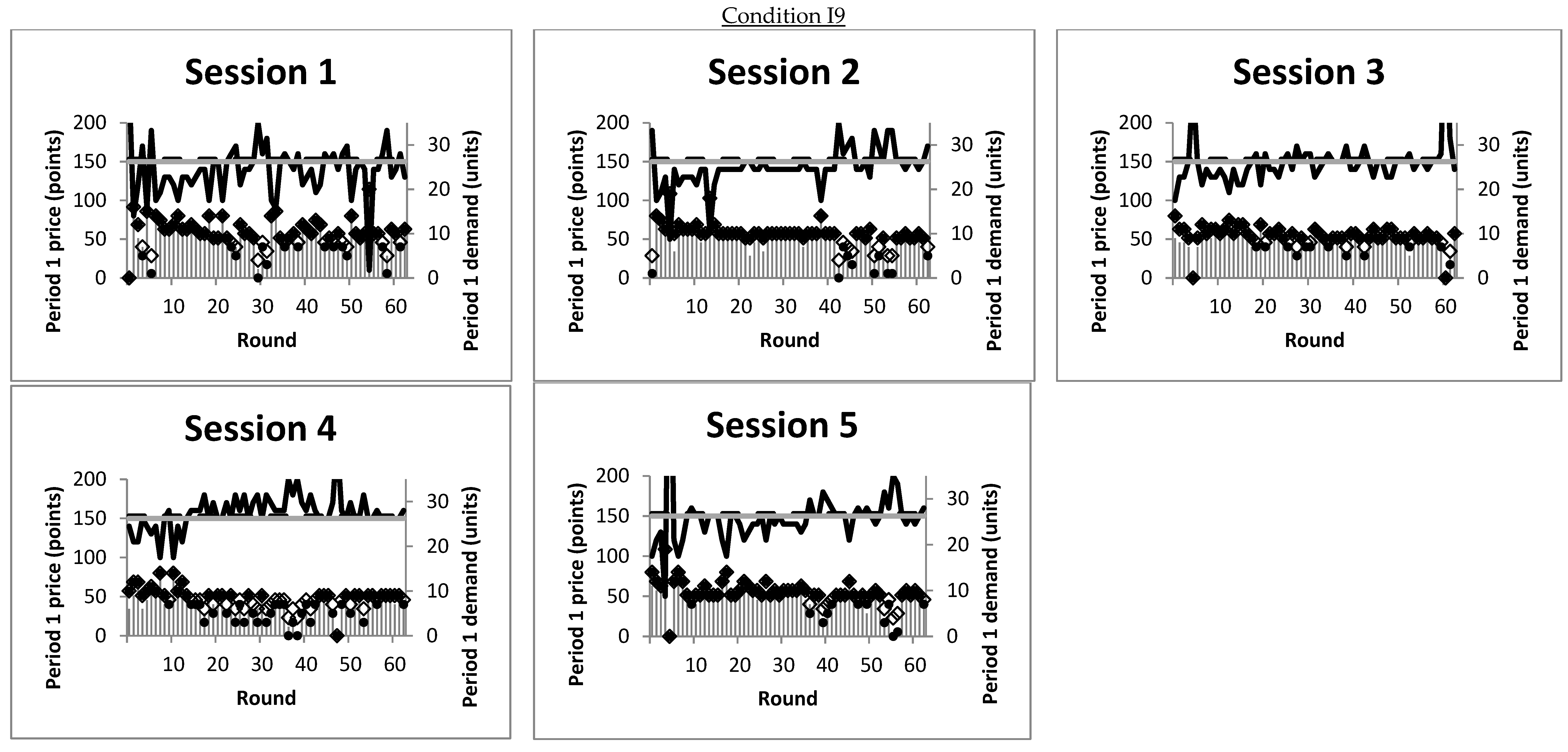
Figure 1, one for each experimental condition, display the price (thick solid line) and demand (gray vertical spike) in period 1 in every round of the 10 sessions; note that “demand” refers to attempted purchases, which might or might not be successful. The equilibrium period 1 price (dashed line) and the one-period optimal selling price (gray horizontal line), as well as the rational expectations equilibrium demand (solid dot) and myopic demand (hollow diamond) in response to the period 1 price, are also displayed as benchmarks. An inspection of the five sessions in each panel suggests that
period 1 prices and demands largely approximated the equilibrium predictions. In Condition I9, the period 1 prices did undergo significant fluctuations (e.g., in Session 1), but the fluctuations were approximately around the equilibrium levels. Equilibrium and myopic demands often coincided in Condition I9, when the realized period 1 demand would typically be the same as the rational expectations equilibrium response to the period 1 price. There was also a significant number of instances (especially in Sessions 3 and 4) where relatively high prices led to rational expectations equilibrium response and myopic demands being different. In those instances, the realized demands were notably closer to the equilibrium than to the myopic benchmark.
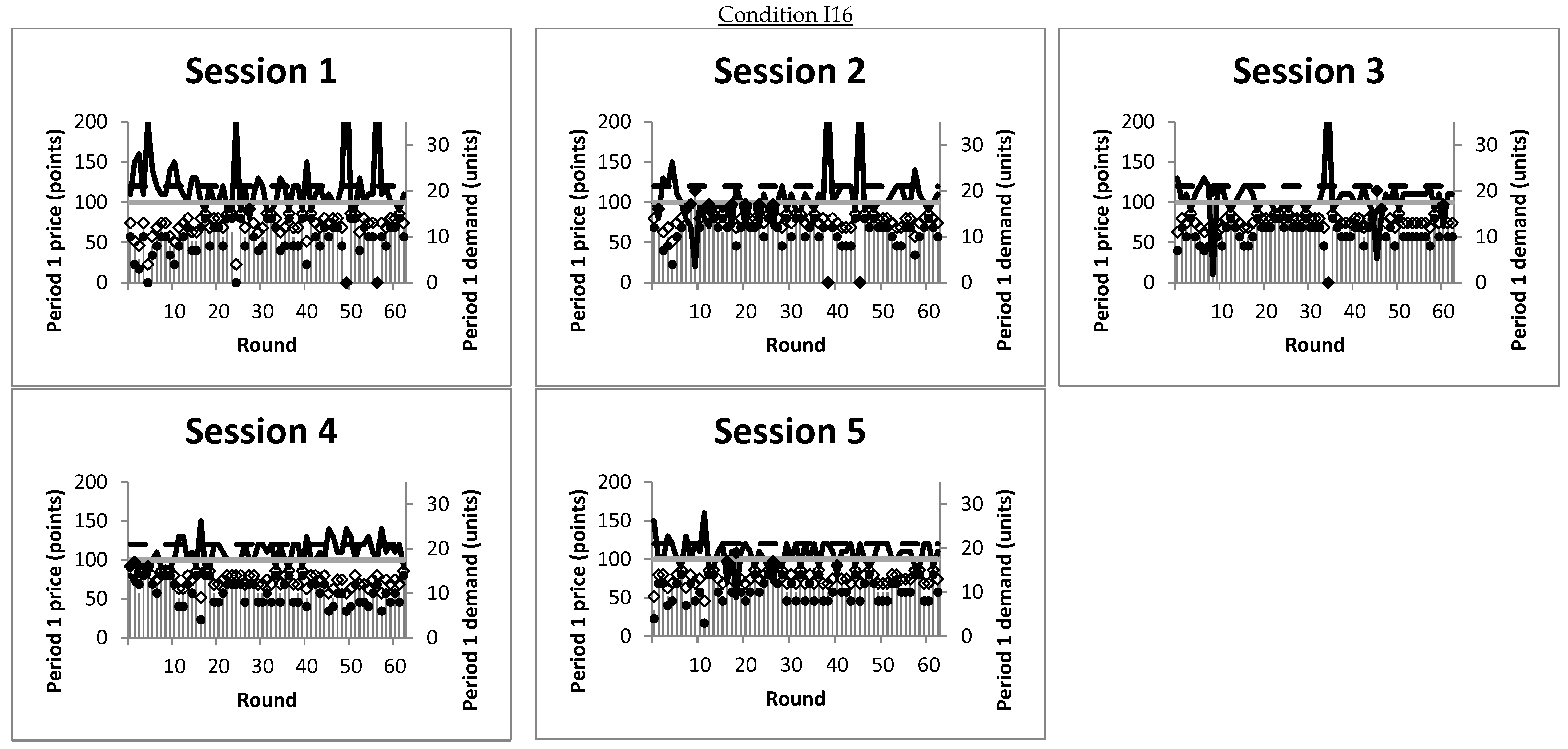
In Condition I16, apart from a minority of instances of very high or very low prices, the period 1 prices generally fluctuated between the equilibrium level and the one-period optimal selling price. In other words, while the period 1 prices were well approximated by the equilibrium prediction, they seemed to be higher than the equilibrium level in general. In the same condition, the rational expectations best response and myopic demand were typically different, and the two panels in
Figure 1 suggest that the realized demand tended to be closer to the best response than to the myopic level.
Further analysis of buyers’ decisions (
Supplementary Online Appendix C) reveals that, at the individual level, buyers were often highly heterogeneous in terms of strategic sophistication. Nevertheless, equilibrium best responses were almost always ex-post optimal for the individual buyer, which is not surprising since the other buyers exhibited high strategic sophistication on the aggregate level.
5.2. Analysis of Pricing Decisions: Boundedly Strategic Behavior among the Sellers
Table 3 presents the means and standard deviations of several major period 1 dependent variables in each condition in blocks of 21 rounds each, where Block 1 consists of Rounds 1 to 21, Block 2 of Rounds 22 to 42, and Block 3 of Rounds 43 to 63. The entries in column 2 of
Table 3 suggest that the period 1 prices in Condition I9 became non-significantly different from equilibrium as the session progressed; by contrast, the period 1 prices in Condition I16 became significantly higher than equilibrium as the session progressed. The table also shows that the seller’s period 1 profits (column 3) were significantly lower than the overall equilibrium in Condition I9, but not different from that in Condition I16; a similar conclusion is obtained regarding the total discounted round profit, with concomitant opposite differences for buyers’ payoffs (see
Table A1 in
Supplementary Online Appendix C).
It thus seems that pricing at equilibrium in Condition I9 did yield as much profit as might have been expected. Nevertheless,
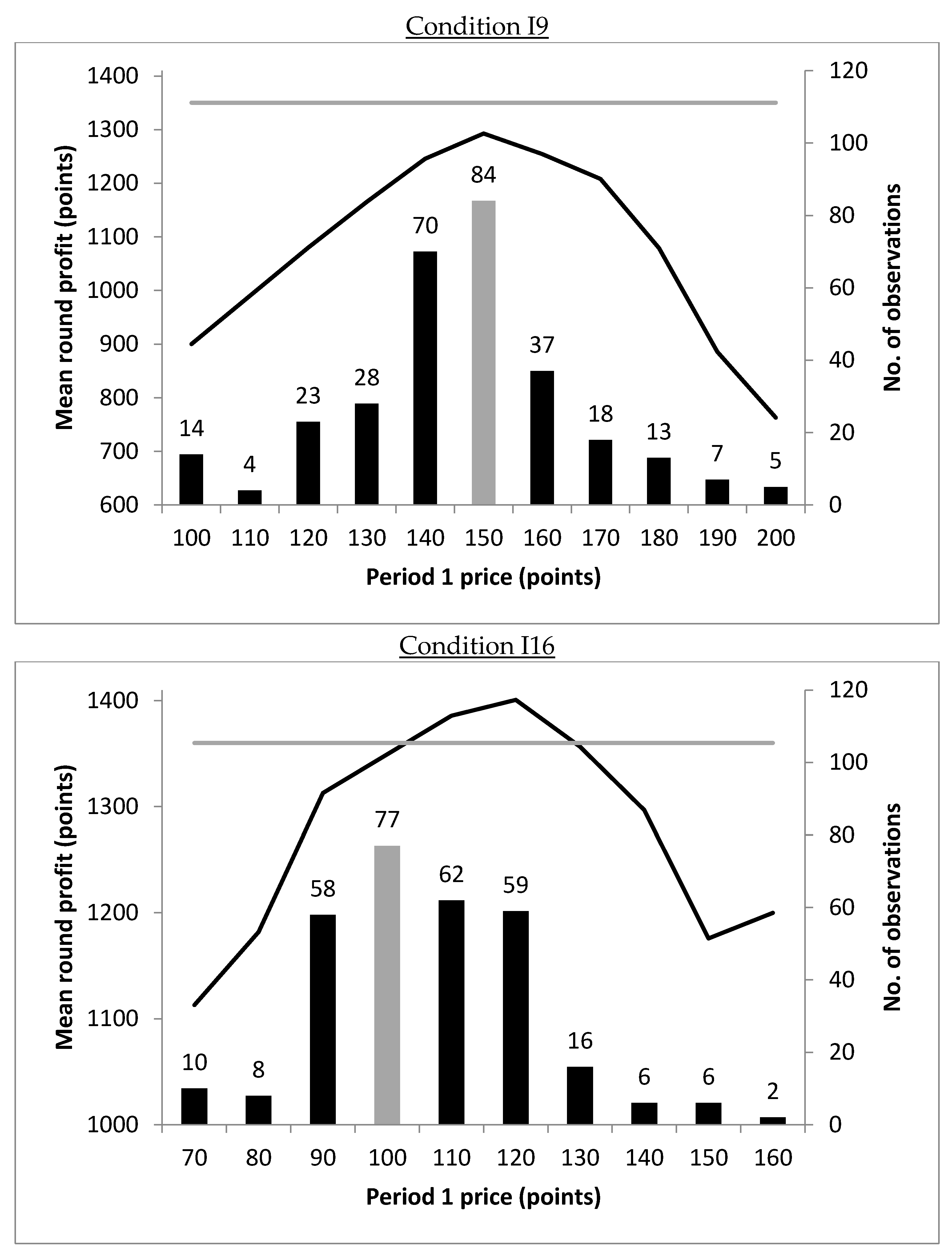
Figure 2 suggests that the ex-post optimal price was often the overall equilibrium price in that condition, and the sellers were often doing the best they could ex-post. The figure includes plots for each condition of the ex-post mean discounted round profits by period 1 price (thick solid line), as well as a histogram of period 1 prices pooled over all players in the same condition (bars). In the panel for Condition I9, the mode of period 1 price was the equilibrium price, which sellers did learn to approach as the session progressed, and did lead to the highest mean ex-post profit as well. That is,
in Condition I9:2 (a) Rounds in which the seller chose the overall equilibrium price in period 1 were, on average, ex-post most profitable; (b) Sellers were often able to price at equilibrium level to capture optimal ex-post profit on average.A different picture emerges for Condition I16. The ex-post optimal price was higher than the overall equilibrium price in that condition; indeed, in the panel for Condition I16 in
Figure 2, the highest mean ex-post round profit, which was higher than the equilibrium level by 3% (1401 versus 1360), was achieved by prices that were higher than the equilibrium level.
3 As it turns out, a majority proportion of 62.9% (198 out of 315) of the observed prices lay over the range of prices {100, 110, 120}, which includes the overall equilibrium level (100) and the ex-post optimal level (120). Specifically, many price observations (158 out of 315, or 50.2% of the observations, including seven outliers not plotted in Figure 4) were higher than the overall equilibrium, which was ex-post more profitable, on average, than the overall equilibrium price. In fact, pricing by the overall equilibrium level yielded an ex-post mean profit of 1349, which was slightly lower than the predicted 1360, and which render pricing at the ex-post optimal level more beneficial (as that would lead to an increase in 3.8% of ex-post mean profit). However, there were also many observations of pricing at the overall equilibrium level (77 out of 315, or 24.4% of the observations), which on average was
not ex-post optimal.
To sum up,
in Condition I16: (a) Rounds in which the seller chose a price of 120 in period 1, which was higher than the overall equilibrium level, were on average ex-post most profitable; (b) Sellers were boundedly strategic, as their prices often exhibited strategic upward adjustments from equilibrium to profit from buyers with limited strategic sophistication, but also often exhibited a bias towards the overall equilibrium price. Additional analysis shows that individual subjects’ mean period 1 prices were highly heterogeneous, with distributions that centered around the equilibrium levels for Condition I9 and just above equilibrium for Condition I16 (
Figure A2, Supplementary Online Appendix C). This finding offers consistent evidence that our aggregate observations above are valid at an individual level among subjects.
5.3. Systematic Deviations in Demand
We now present an analysis of buyers’ response to the posted prices, which allows us to understand the ex-post optimal price levels reported in
Section 5.2.
Deviations in period 1. To analyze the observed demands in period 1 as buyers’ collective responses to the observed period 1 prices, the meaningful benchmark is not the overall equilibrium demand (the demand given the overall equilibrium price along the gray rows of
Table 2). Rather, it is the rational expectations equilibrium best response demand, given the period 1 price—that is, the entries in the second column in
Table 2 as a function of the corresponding period 1 prices. As is apparent in
Table 2, the best response demand is not constant with the period 1 price. It decreases/increases as the period 1 price becomes higher/lower, as with a standard demand function. Our finding from
Table 3 is that the observed period 1 demands (column 4 of
Table 3) were largely best response to the period 1 prices (column 5 of
Table 3), except in Block 1 of Condition I9 and Block 3 of Condition I16.
The demand observations from
Table 3 may be visualized in
Figure 3, which together with
Figure 4 shed light on the strategic interactions between the single seller and the multiple buyers in intermediate stages of the game.
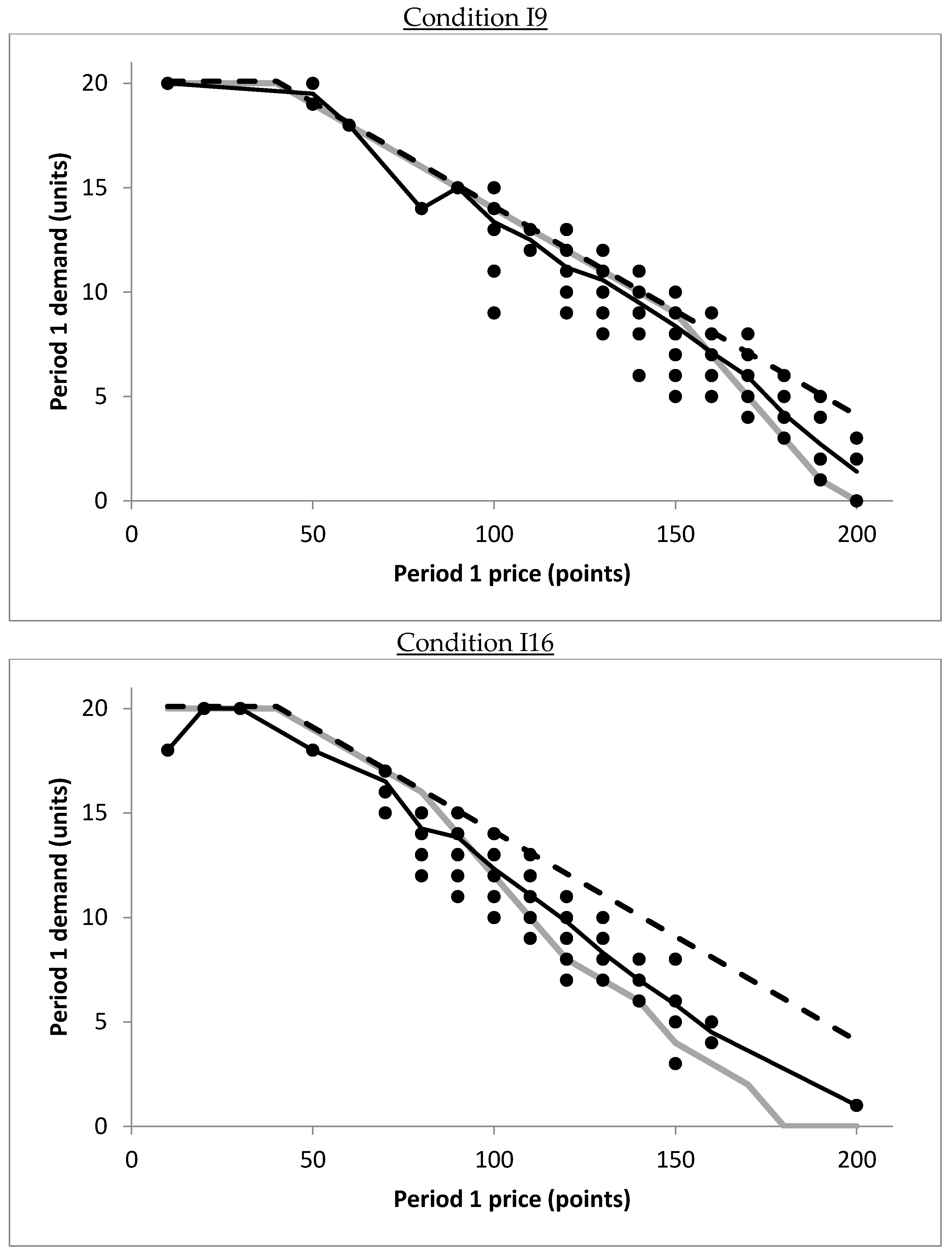
Figure 3 displays period 1 demands as responses to the period 1 price separately for each condition; it is clear from the two panels in the figure that the demands tend to cluster around the best response equilibrium levels rather than the myopic demands. The figure suggests that the buyers were, on the aggregate, strategically sophisticated. However, there are also nuances of deviations in both conditions:
period 1 demand tended to be higher (lower) than rational expectations best responses at high (low) prices relative to the equilibrium level. To put in another way, the observed demand did not change as much as the best response demand at prices around the equilibrium level, so that it was lower/higher than the best response when the price was lower/higher than equilibrium.
To be more precise, in the panel for Condition I9 the mean and best response demand cross at around price = 160, which is slightly higher than the equilibrium level of 150; in the Condition I16 panel, the mean and best response demand cross at around price of 90, which is slightly lower than the equilibrium level of 100. To obtain statistical support for these observations, we compared the mean demand deviation whenever the period 1 price was lower than 160 in Condition I9 and 90 in Condition I16, and found that the deviation was indeed significantly negative according to
t tests in both conditions (
p < 0.05 in both tests, with session as the unit of analysis). Likewise, the mean demand deviation whenever the period 1 price was higher than or equal to 160 (90) in Condition I9 (Condition I16) was significantly positive according to similar
t tests (
p < 0.05 in both tests). These results are consistent with the findings reported in [
13] that, at sufficiently high levels of scarcity such as those in our experiment, period 1 demand deviated positively (negatively) from the best response at high (low) prices.
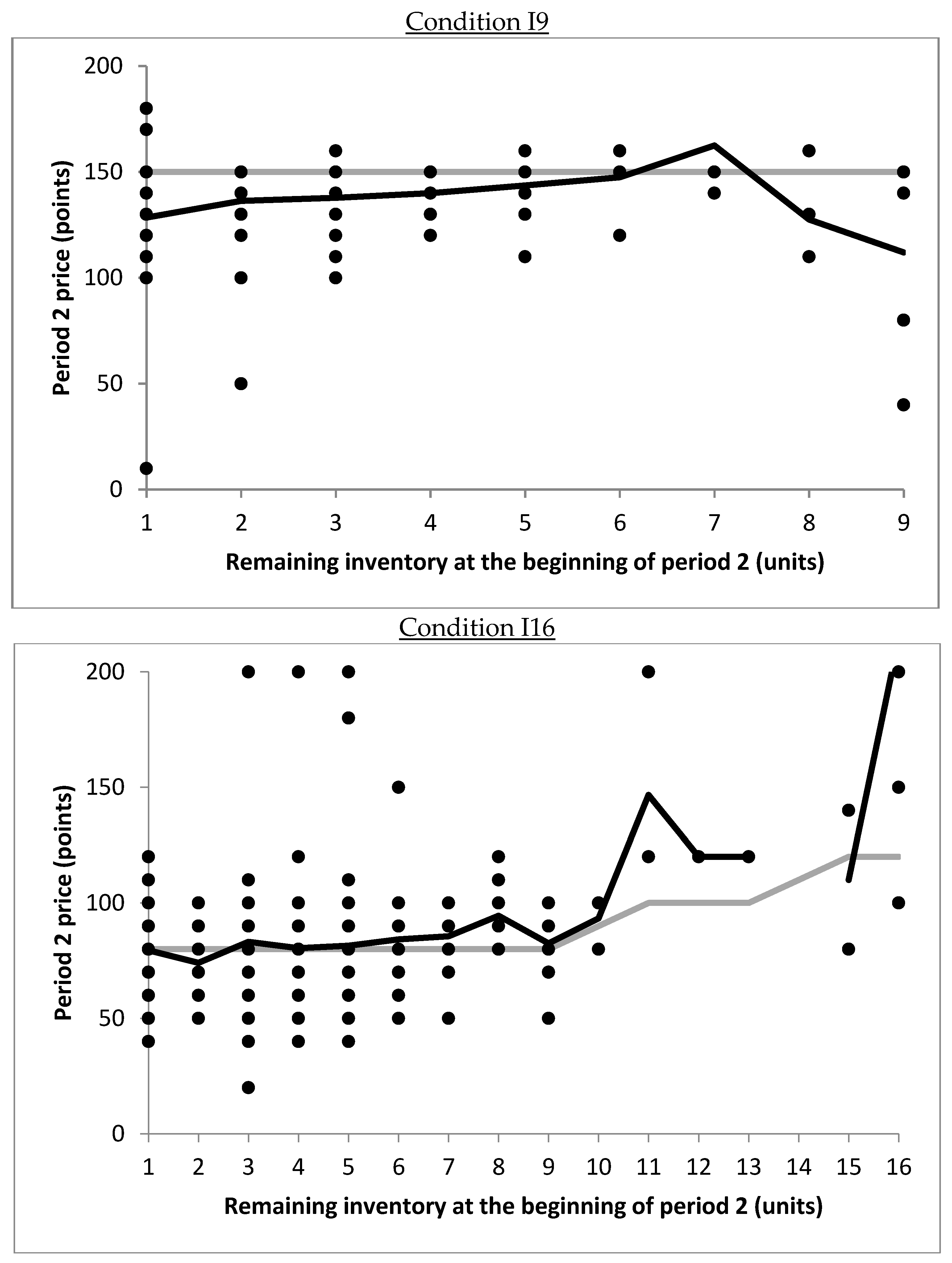
Deviations in period 2. We conclude this subsection with a discussion of the deviations in period 2. For rounds that proceeded to period 2,
Figure 4 displays the period 2 prices as responses to the remaining inventory at the beginning of that period. The figure shows that most observations cluster around the optimal period 2 prices (gray line) in each panel. We find that, with Condition I9, the period 2 prices are significantly lower than optimal by 15.8 on average (
t test yields
p < 0.01). Note, however, that only 42% (132 out of 315) of the rounds in Condition I9 proceeded to period 2, compared with 95.9% (302 out of 315) in Condition I16. Meanwhile, on average, the period 2 prices were 3.66 points higher than their optimal levels in Condition I16, a difference that is not significantly different from zero according to a
t test with session as the unit of analysis (
p > 0.19).
5.4. The Relationship between Deviations in Demand and the Ex-Post Optimal Price Offer
As reported in
Section 5.3, in Condition I16 (but not in Condition I9) demands at high prices in period 1 tended to be significantly higher than theoretical predictions. The seller could price higher than prescribed by our equilibrium analysis to capitalize on the demand deviations. Accordingly, the ex-post optimal price in that condition exceeded the equilibrium (
Figure 2).
To further understand the differences in ex-post optimal prices across conditions, we examine the differences in opportunities for myopic buying between them. Myopic buying occurred when a buyer attempted to purchase in period 1 while
v** >
v >
p1,
v being her valuation and
v** being the cutoff valuation for best response purchases as defined for
Table 2. That is, the buyer
should not have attempted to purchase even though her valuation is higher than the period 1 price, since the equilibrium prescribed that the buyer should wait strategically as a best response; myopic buying occurred when this occasion arose and the buyer “attempted purchase myopically” vis a vis considerations of rational expectations.
The deviation between ex-post optimal and equilibrium prices in Condition I16 was due to positive bias of demand at high price, which could only be driven by myopic buying behavior. As such, there are few opportunities for myopic buying deviations at prices around equilibrium in Condition I9 compared with Condition I16, as reflected in the numbers of buyers in each case who would wait strategically in equilibrium (
Table 2, column 5). Hence, the deviations between ex-post optimal and equilibrium prices became correspondingly insignificant in Condition I9. The implication is that a seller in our experimental setting would find it most profitable behaviorally to price higher than the equilibrium assuming fully strategic buyers, when (a) there is a sufficiently high extent of scarcity and the equilibrium price is sufficiently high, but (b) a sufficiently large number of buyers would wait strategically in equilibrium. The two conditions define the boundary conditions for the deviation of ex-post optimal price from equilibrium.
5.5. Learning Analysis
We end
Section 5 with a discussion on evidence of learning in our experiment.
Sellers. Table 3 (column 2) and
Figure 1 suggest that there was a prominent increasing trend with period 1 prices in the experimental sessions in Condition I9, but the same cannot be said about Condition I16. To examine these observations statistically, we conducted for each condition a three-factor within-subject ANOVA with period 1 price as the dependent variable, block as the within-subjects factor, and session as the unit of analysis. Consistent with
Table 3 and
Figure 1, we find a significant effect of block with Condition I9 (
F(2,8) = 5.98,
p < 0.05) but no such significant effect with Condition I16 (
F(2,8) = 1.00,
p > 0.4). Moreover, both
Table 3 and
Figure 1 suggest that the increasing trend in Condition I9 started with prices that were lower than equilibrium, which eventually rose to around equilibrium level; meanwhile, prices in Condition I16 were often higher than equilibrium. That is:
(a) Sellers in Condition I9 learned to increase their period 1 prices towards the equilibrium level as the session progressed; (b) Sellers in Condition I16 set their period 1 prices around levels that were higher than equilibrium from early on in the session. An implication of these results is that sellers apparently remained boundedly strategic throughout the session in Condition I16, where the ex-post optimal price and overall equilibrium price differed; but they gained strategic sophistication over the session in Condition I9, a condition in which the two prices coincided, rendering optimal decision making arguably simpler to intuit.
Buyers. We next examine if subjects in the role of buyers learned to reduce the two types of deviations as the session progressed. A meaningful analysis might only be carried out after accommodating possible confounds due to systematic changes in the seller’s pricing decisions over the session, since deviation tendency could differ significantly with prices over and above learning effects. To proceed, we first isolate instances in which a buyer might exhibit myopic buying (i.e.,
v** >
v >
p1 as discussed previously); we then carry out a logistic regression over these instances for each condition, with the likelihood of myopic buying as the dependent variable and the period 1 price, the round number, and the interaction term (period 1 price × round number) as the three independent variables. We use the generalized estimating equations (GEE; see [
41]) approach in the regression to account for possible dependencies among observations from the same subject or the same session. As it turns out, in Condition I9 the estimated coefficient (standard error in parentheses) for round number is −0.40 (0.16), and that for the interaction term is 0.0022 (0.0009); both coefficients are significantly different from zero at
p < 0.05. Note that, except in rounds where period 1 prices were higher than 180 (which constitute only 17 of 315 observations), the positive interaction effect could not overturn the negative round number effect; hence, in general, the buyers were less prone to myopic behavior as the session progressed, controlling for the period 1 price. The corresponding estimations for Condition I16 are not significantly different from zero (
p > 0.8 for both coefficients).
A similar GEE logistic regression for the opposite type of deviations, namely, irrational waiting, shows similar results (irrational waiting occurred when the buyer did not attempt to purchase in period 1 while
v >
v**; see “irrational demand withholding” in [
22,
23]). In Condition I9, the estimated coefficient (standard error in parentheses) for round number is −0.15 (0.03), and that for the interaction term is 0.0008 (0.0002); both coefficients are significantly different from zero at
p < 0.01. As with myopic buying, unless at prices that were higher than 180, the overall effect was lower likelihood of irrational waiting as the session progressed, controlling for the period 1 price. The corresponding estimations for Condition I16 are not significantly different from zero (
p > 0.15 for both coefficients). To sum up:
(a) As the session progressed in Condition I9, buyers became more strategically sophisticated vis a vis both myopic buying and irrational waiting deviations; (b) In Condition I16, learning among buyers was not significant.It needs to be emphasized that our subjects learned to reduce both types of deviations in Condition I9. The implication is that the deviations remained likely to mitigate each other consistently throughout the session, so that the aggregate behavior of the buyers remained close to the rational expectations equilibrium.
6. Conclusions
Pricing strategies are a critical component in revenue and logistics management and must dynamically adjust to inventory changes over time. This picture is further complicated by the fact that on the demand side are buyers who might attempt to pre-empt any dynamic pricing policies. The resulting strategic interactions are the central concerns of the present research.
In this study, we examine how human (rather than simulated) sellers set prices and interact with human buyers in an experimental setting using dynamic pricing under capacity constraints. We report important systematic patterns in sellers’ pricing strategies and buyers’ responses. To sum up our major results:
Period 1 Seller’s prices and Buyers’ demand largely approximated equilibrium predictions. However, at a more nuanced level, Period 1 demand tended to be higher (lower) than the rational expectations best responses at high (low) prices relative to the equilibrium level.
In Condition I9 (high capacity constraint; low capacity):
- (a)
Sellers were often able to price in period 1 at equilibrium level, which captured optimal ex-post profit on average;
- (b)
As the session progressed, the sellers learned to increase their period 1 prices towards the equilibrium level, while the buyers generally became more strategically sophisticated vis a vis both myopic buying and irrational waiting deviations.
In Condition I16 (relatively low capacity constraint; high capacity):
- (a)
On average, the ex-post most profitable price in period 1 was higher than the equilibrium level. The sellers were boundedly strategic, as their prices often exhibited strategic upward adjustments from equilibrium to profit from the buyers with limited strategic sophistication, but also often exhibited a bias towards the overall equilibrium price;
- (b)
From early on till the end of the session, the sellers set their period 1 prices around levels that were higher than equilibrium; learning among the buyers was not significant.
Importantly, by examining interactions between human decision makers on both supply and demand sides, our work complements related studies such as [
9] on sellers’ dynamic pricing responses to a simulated market of buyers, and [
13] on buyers’ responses to a simulated seller in a dynamic pricing context.
As our analysis suggests, the sellers’ deviations often seemed to be strategically sophisticated attempts that enabled them to profit from the buyers’ deviations from equilibrium purchase. This lends further support to the applicability of the findings of [
13] in practical situations with human sellers as well as buyers. Our finding is also consistent with the fact that behavioral operations studies often reveal suboptimal decision patterns (see, e.g., [
11,
12]), since the sellers in our experiment appeared to be boundedly strategic: when the equilibrium and ex-post optimal prices were different, the sellers’ prices seemed to be “torn” between the ex-post optimal and a bias towards the overall equilibrium. Our specific observations of ex-post profitable over-pricing relative to equilibrium contrast with the finding of [
16] of underpricing in a comparable dynamic pricing experiment without inventory constraints; the contrast highlights the important impact of scarcity in sellers’ decisions. Meanwhile, aggregate demand
largely approximated our predictions assuming fully strategic buyers, despite nuanced systematic deviations. These results on the demand side are in line with those of empirical studies such as [
19,
20,
34] on essentially aggregate data.
As with most laboratory experiments, our study has examined decisions in a highly stylized environment, and our conclusions are based on conditions involving a small set of parameter choices. However, our experimental setup has the crucial advantage that it allowed us to directly isolate and test individual deviations from rational expectations benchmarks that are point predictions; consequently, we may obtain the insights reported in the present paper. These insights offer several practical implications:
Firms’ dynamic pricing strategies should not always be formulated as if the consumer market is highly strategic, nor as if the market is highly myopic. When there is a high capacity constraint, it is probably optimal or near-optimal to assume that the market is highly strategic. However, with lower capacity, assuming that the market is highly strategic (just like assuming that it is highly myopic) might lead to suboptimal profits. Firm decision makers should avoid falling into the trap of over- or underestimating the consumer market’s strategic sophistication.
The consumer market may exhibit high (though potentially limited) strategic sophistication in correctly expecting potential future discounts, even if individual consumers might appear to be unsophisticated. At a more nuanced level, the market might adjust demand upwards less than it should when the price is low and adjust demand downwards less than it should when the price is high. This indicates that individual consumers could improve in savviness in terms of pre-empting potential future discounts.
Future Directions
Several future theoretical and experimental directions are warranted. First, our descriptive findings may contribute towards a comprehensive behavioral theory on dynamic pricing (see Baucells et al. [
18] for a recent example). While our observations of sellers’ pricing decisions conform to a boundedly strategic view, it is worthwhile to further explore how the limits in strategic sophistication came about: what heuristic rules and decision-making biases could be putting such limits on sellers’ decision optimality? Secondly, the behavioral anomalies discussed in this study may be affected by the proportional rationing scheme used to assign the goods when demand exceeded supply. Other rationing schemes might be considered for future research, such as assignment according to an exogenous hierarchy. Since different rationing schemes might lead to different probability (real or perceived) that a buyer would succeed in a purchase attempt, they might create significant differences in behavior. Thirdly, more experimental conditions might be performed with the present setup to explore new behavioral phenomena. These include, for example, a very high level of inventory that would lead to leftover after period 2 in equilibrium (see the Type II two-period equilibria in
Table 1), or the seller having a higher seller discount factor than the buyers.
It is also potentially worthwhile to go beyond the monopolistic context and consider how competition between sellers interacts with dynamic pricing, strategic players, and inventory; relevant studies along this line, but without inventory issues, include [
35,
36]. Another important extension possibility is that the seller may endogenously make inventory decisions before the market opens. It can be shown that the inventory level in our model that yields optimal profit is generally a moderate value, even when it is costless to stock inventory. The intuition behind is that a moderate level of scarcity makes the best tradeoff between generating sales for profits and discouraging strategic waiting in the first period. Thus, a natural next step is to incorporate endogenous inventory decision into the present framework and examine if seller subjects choose inventories optimally.
Finally, in the model analysis we have assumed that the discount factors are bounded between 0 and 1, and that the discount factor of the seller is greater than that of the buyers. These assumptions should be appropriate in contexts with price skimming; however, they might not hold in some other cases, such as airlines/hotel booking, when fares are not refunded and consumers might prefer to book later if they bear a risk of rescheduling a trip. Another key assumption is that the same buyers participate in the two periods—that is, no new buyers enter the market in period 2. This assumption rules out some interesting cases of dynamic pricing strategies, such as those in the context of flight ticket, car rental, and hotel room rates, which may have prices increasing with time up to the check-in date. These limitations of the present work offer yet additional future directions for research.


 ) and demand (gray vertical spike
  ) in period 1 by round and experimental session. Note that “demand” refers to attempted purchases which might not be all successful. Isolated outlier observations of prices above 200 units (five in each condition) have been excluded. The gray horizontal line (
 ) and dashed line (
 ) indicate, respectively, the equilibrium period 1 price and the optimal price for one-period selling. Each solid dot (
 ) indicates the demand if all buyers followed the rational expectations equilibrium given the period 1 price, while each hollow diamond (
 ) indicates the demand if all buyers were myopic. Where the two coincide, a solid diamond can be observed.


 ) and number of observations (bars
  ) by period 1 price. Gray line (
 ) indicates overall equilibrium round profits and gray bar (
 ) indicates the overall equilibrium price. In each panel, the range of prices on the horizontal axis captures more than 96% of the observations (303 and 304 out of 315 observations in Condition I9 and Condition I16, respectively); the ex-post mean discounted round profits with prices outside the range are all lower than with those inside the range.

 ) by period 1 price and experimental condition. Isolated outlier observations of prices above 200 units (five in each condition) have been excluded. Also exhibited are the mean observed period 1 demand (thick solid line
  ), rational expectations equilibrium demand (gray line
  ), and myopic demand (dashed line
  ), by period 1 price.

 ) by remaining inventory at the beginning of period 2 and experimental condition. Isolated outlier observations of prices above 200 units (two in Condition I9 and three in Condition I16) have been excluded. Also exhibited are the mean observed price (thick solid line
  ) and the benchmark optimal period 2 price (gray line
  ) by remaining inventory (see also Table A in Supplementary Online Appendix A). Note that, in equilibrium, the market should not have reached period 2 in Condition I9, and should have reached period 2 with four remaining units in Condition I16; also, in the Condition I16 sessions, no round had a period 2 with 14 units of remaining inventory, and hence there are no corresponding price observations.

