Abstract
Supply chains for goods that must be kept cool—cold chains—are of increasing importance in world trade. The goods must be kept within well-defined temperature limits to preserve their quality. One technique for reducing logistics costs is to load cold items into multiple compartment vehicles (MCVs), which have several spaces within that can be set for different temperature ranges. These vehicles allow better consolidation of loads. However, constructing the optimal load is a difficult problem, requiring heuristics for solution. In addition, the cost determined must be allocated to the different items being shipped, most often with different owners who need to pay, and this should be done in a stable manner so that firms will continue to combine loads. We outline the basic structure of the MCV loading problem, and offer the view that the optimization and cost allocation problems must be solved together. Doing so presents the opportunity to solve the problem inductively, reducing the size of the feasible set using constraints generated inductively from the inductive construction of minimal balanced collections of subsets. These limits may help the heuristics find a good result faster than optimizing first and allocating later.
1. Introduction
Supply chains that move perishable products such as food and other kinds of products as well are often termed cold chains. Currently there is much interest in improving the reliability of cold chains because quality at the destination requires the successful management of conditions other than simply on time delivery and cost. One cost saving approach to the transport of goods in any supply chain is consolidation of shipments of several customers into a single vehicle. Consolidation is hard enough with simple packaged products such as manufactured goods or typical UPS packages [,]. However, in the case of cold chains, other parameters such as the temperature must be considered as well. For instance, a pallet of lettuce and a pallet of ice cream cannot be moved in the same temperature conditions, and hence they might not be placed together in a truck whose temperature is controlled to protect the ice cream. These constraints limit the mixing of the cold goods, which radically changes the feasible solution space for a typical optimization problem for consolidating shipments. The advent of the “Internet of Things” in transportation introduces the possibility of measuring other parameters while in transit, such as shaking or exposure to chemical agents or moisture, in addition to temperature. These, too, may restrict the solution space of a consolidation plan.
One proposal to deal with the temperature problem for consolidation in cold chains is to use a multiple compartment vehicle (MCV), which, instead of a single temperature controlled space, has several compartments each with separate temperature control, set to different ranges. Such an MCV might allow the transport of several types of goods for several customers in the same vehicle. This kind of transport mix would have special relevance in last mile distribution, perhaps to a number of smaller retailers, who could receive a mix of products in one truckload rather than needing several different deliveries for each temperature range of product. Such vehicles are being studied and produced in Europe. In the US they are exemplified by home delivery cold chain retailers such as Schwan’s, a firm that delivers cold products to individual consumer homes on a subscription basis. Design of such vehicles on a 40 foot or 53 foot container scale could make a large difference in consolidation costs in longer distance transport, including ocean transport.
Much of the study of multiple compartment vehicles is done in the scenario of liquid delivery such as petroleum or propane. One difference in the cold chain is that the units shipped have three dimensions as well as weight. This makes the MCV loading problem more difficult since it involves packing objects of defined shape into a rectangular solid space—a more difficult packing problem than simply filling a tank. In this paper we discuss the MCV problem as an mathematical program to compute a good (here meaning low cost) plan for stowing a number of units of products which differ in ownership and temperature range allowed as well as size, weight and density. The typical problems constrained by size, weight and density alone are already hard in complexity, being extensions of bin packing problems, which are a form of generalized assignment problem. They are normally solved in real cases using heuristics, which must return a feasible solution (one that can actually be used to load the truck) at all times, and somehow improve the cost as they go along; though perhaps taking false directions as they advance, they must not stop without reporting a solution that can be acted on. The extra constraints on the temperatures make the computational problem much more difficult.
Another aspect of the problem is the fact that in less-than-truckload transport several cargo owners are sharing the same vehicle. The immediate question once we have found a ’good’ loading plan, is how should the cost be divided among the individual owners?
An example of the difficulty is present in typical package or less-than-truckload (LTL) delivery or air freight today. As packages differ in dimensions, weight, and density, many carriers have moved to a so-called dimensional weight or ’dim weight’ basis for pricing shipments. Machines have been invented which scan a package or unit and weigh it, and compute a number which is used as a basis for the charges. Many LTL carriers have installed these at their loading docks, and process all units through it before determining the pricing or loading of the vehicle. UPS, which sells substantial shipping online, must provide pricing in advance of such measurement. On its website, UPS requires specification of three dimensions and weight, (plus some nonspecific information like irregular shape), and calculates a number they call ’dimensional weight’ or ’cubed weight’ (measured in pounds) which is then used as the basis for computing price along with distance to move and handling required or other so called accessorial charges. A study showed that air freight load capacity utilization by weight was too low by 25% for the industry [].
The principal advantage of dim weight costing and pricing is that package deliveries often cube out well before they weigh out; the packages tend to be light and take up space. The dim weight calculation takes the volume of the package and divides it by a preordained density factor to get the dim weight. The number used today is typically 166 cu in/lb for dimensions in inches and weights in pounds, for UPS large packages, DHL and for IATA air transport; 139 for UPS and Fedex; or it can be whatever the carrier sets. The figure corresponding to 166 cu in/lb is 5000 for rectilinear dimensions in centimeters and weights in kg. Carriers can adjust the factor so that they translate package size to a sort of standard weight reflecting the density of load they wish to carry (figures obtained as of 1 March 2018 from websites of carriers).
The problem with such single measures for pricing or costing is that a truckload can on occasion weigh out (reach a weight limit before the space is filled—often called ’shipping air’), or cube out (the space is filled well before the weight limit), or load out (the load becomes unstable and might shift or damage units inside because of very dense or odd shape units which must be loaded precisely. The last is often seen in project cargo such as large machines, tanks, or steel shapes. An extra truck might be required even though the goods would fit on a dimensional weight basis. The pricing by dimensional weight would not reflect accurately the actual cost of shipping.
The question of cost allocation to customers is also relevant in the MCV problem, perhaps more so, because the additional parameters of the shipment, specifically the temperature range required to be maintained, is much harder to factor into a single cost number. In the case of Schwan’s deliveries mentioned above, the problem is harder to see, because the units being shipped all have one owner. However, we still internally have the issue of cost allocation to the specific products in order to obtain the full activity-based cost of delivering the product.
In Reference [] authors reviewed the literature on cost sharing in collaborative transportation. One method of analyzing cost allocation in general and particularly in transport, is cooperative game theory. Framing the allocation problem as a cooperative game is normally done by assuming that we have an algorithm to determine the optimal cost of any mix of units (for instance, []). The cooperative game problem then uses the costs of each possible subset of units to discover solutions—cost allocations to the units’ owners. A cost allocation is said to be stable if it has additional properties that make it desirable to actually use to charge unit owners. Some of these are outlined in Section 3 below. These are derived from the extensive literature on cooperative game theory. But this two-step method (determine cost first, then allocate it) is less suitable when the cost must be calculated via a heuristic. We don’t know that the cost is the minimum, and therefore our conjectures about dividing it ex-post fairly could be thrown off.
In this paper we propose that the MCV problem needs to be solved in concert, simultaneously, with the cost allocation problem. While we assert that this could be true for any optimization cum cost allocation exercise, the great complexity and heuristic nature of the MCV problem makes it both essential and valuable to solve them together. In this paper we propose a strategy to do this, by using the cost allocation game to generate additional constraints that help streamline the calculation of the heuristic by bounding the solutions. The process we propose is inductive on the number of unit owners (customers). We specify it in Section 5 after discussing the inductive construction of the balancing conditions in Section 4. We leave open the question of what heuristic is used by the analyst; our goal is simply to set forth the paradigm for solution. It is sometimes asserted that it is impossible to solve for a cost the MCV loading problem independent of the vehicle routing (VR) implied by the loading. We will skirt this problem by leaving out the VR problem.
Many papers have been written recently offering heuristics for solving one version or another of the MCV problem, with different constraints, as the problem of last mile transport grows more relevant in logistics. For instance, [] worked on a simplified version involving putting packages on standard pallets, and pallets into trucks in specific layers. They included geometric constraints with some limitations, rather than 3D packing, and they studied the effect on solutions of overall weight, weight per axle, center of gravity of cargo and dynamic stability. Each in turn produced fewer exact solutions and more approximate ones. They extended their method to requiring special configurations for packing or for unloading sequence. Their integer program achieved many optimal solutions for this restricted version. Reference [] developed a three-dimensional algorithm using a multi-population biased random key genetic algorithm (BRKGA) heuristic to pack boxes of varied sizes into a single container, with either full support on all sides, or with support only on the bottom. Their heuristic performed better than 13 others as measured on 1500 problems using the percent of total packed volume. The article contains a nice summary of the types of algorithms previously considered. Another example of a heuristic is [], who used a GRASP heuristic to solve the 3D bin packing problem with variable size bins; they coupled it with a Path Relinking procedure for the best solutions. Authors [] add axle weight constraints, and confine themselves to sequence-based loading, in which the packages need to be loaded in a sequence. This is again a special case. They use an iterated local search algorithm, which includes a vehicle routing problem dependent on the loading sequence. Reference [] solves a container (compartment) loading problem with sophisticated constraints for static mechanical equilibrium. This protects cargo from shifting front to back or side to side in a compartment. They show how the loading problem depends on the codification of a loading pattern. Their solution uses a BRKGA. Reference [] treat the container loading problem as a 3D knapsack integer programming problem, with each package having a ’size’ and value, maximizing the value loaded (represented by the percent of volume loaded), subject to cargo stability constraints (how much is the base supported) and load bearing constraints (how high can they be stacked), as well as all the constraints needed for packing in three dimensions. They limit compute time to an hour, and see how far they can get on 320 randomly generated problem instances.
Many more examples could be cited. The point is that heuristics specific to the particular loading problem are required, in general a formulation does not capture exactly all the loading issues, and some constraints cannot be evaluated till after the load is completed, complicating the approach. Practitioners addressing specific problems will need to determine the heuristic they consider best suited to a practical solution. What we are trying to do here is to demonstrate a procedure for adapting any heuristic for loading to assure that the outcome also admits a fair and stable allocation of the costs associated with the load. This can be accomplished by solving the problem in an inductive manner using the algorithm of choice, adjoining appropriate constraints on the cost deriving from the costs of the partial loads (the subsets).
The paper is structured as follows. Section 2 defines the multiple compartment vehicle (MCV) problem, and remarks on some solution difficulties. We then embed the problem in a more natural comprehensive one. Section 3 introduces cooperative games, and stable cost allocations. We present Peleg’s [] notion of inductive construction of minimal balanced collections of subsets. Section 4 investigates how inequalities for a specific configuration of items can be constructed inductively from the minimal balanced collections. Section 5 outlines the algorithm that might be employed in conjunction with some heuristic to solve the MCV problem. Section 6 gives a brief example applying the method. Section 7 summarizes our results and offers some suggestions for future investigation.
2. The MCV Problem and an Extension
The basic unit of transport we shall term the vehicle, though it could be a container or portion of a warehouse. We shall index vehicles by the index , though at first we will discuss only a single vehicle. Each vehicle has a weight limit which may not be exceeded. It is calculated in real weight units, not dim-weights. A vehicle is divided into compartments or cells, labeled by . Each cell c has a list of properties Some of these are shown in Figure 1 below. There could be other properties of a cell added, but the ones germane to our case are the length , width , height , minimum temperature , and maximum temperature . The cell can be set to maintain any temperature between the minimum and maximum temperature, but the cost of operating it is a function of the coldness set, a decision variable for the cell. This function must be specified—in the simplest form one could assume linear dependence with slope in dollars per degree below the maximum the compartment is set at. The cost is problem specific of course and would be determined by analysis.
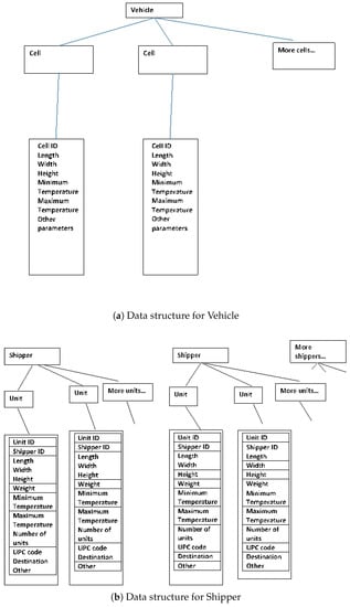
Figure 1.
Data structures for Vehicle and Shipper.
A shipper is an entity or firm that consigns something to be loaded into the MCV. Shippers are denoted by . One can think of what is loaded as a package with a variety of attributes. We shall borrow from the packaging industry and use the term unit for the item consigned by the shipper. Unitizing products in logistics packaging means packaging them for shipment in a manner designed to ship well, protect against damage, and group them in a desirable quantity for delivery. Typical unitizing might be a stack of identical packages on a standard pallet, shrink wrapped in plastic, and possibly padded, for protection and to keep the load together in handling. Other forms of unitization include shipping cartons in which multiple units of rectangular solid shape are precisely packed so as to leave no unfilled space. While in the cold chain there can be cylindrical packages, such as for bulk ice cream, in general packages are unitized into a more or less rectangular solid shape. We therefore assume that a unit is characterized by a length , width , and height , as well as a weight .
The corresponding dim-weight is computed from the size and weight data, and will be denoted by . In addition there are a minimum temperature , maximum temperature , and target temperature ; the unit should be transported at the target temperature, and the actual temperature must not be outside the min-max interval specified. A unit also has a universal product code (UPC) code, some barcode marking that allows determination of the nature of the shipment; this will not be used in the optimization. We prefer to use the temperature control data directly specified in the optimization, though in many cases this could be indirectly specified by using the UPC code as a pointer to the actual temperature data for this product. In the data structure for a unit we explicitly maintain the shipper’s identity. We also carry the destination of the unit. This may or may not be the same for all units owned by a single shipper. The destination may or may not play a role in the packing problem cost; it could influence which items were to be loaded or the order loaded or unloaded. We do not intend to use the destination in our outline of a solution method.
In the math programming model we will be trying to load specific units u into cells c which fit, do not exceed the weight limit for the vehicle, and so that the cell temperatures can be set to maintain the units within the limits of each one in that cell. We will also use the information on the shipper of a unit to attribute cost properly to the shippers based on what they have shipped in some way.
Decision variables for the MCV problem include binary variables , which are 1 if unit u is placed into cell c and 0 otherwise. The binary variable is 1 if cell c is used, i.e., if at least one of the for cell c is 1.
A specific packing or choice of the X’s, is also constrained by cell temperature and unit temperature limits, so that cell temperatures for operation must also be chosen to be compatible with the items packed. It is also constrained by an overall weight test; the sum of the weights of the units in all cells must not exceed the weight limit of the vehicle. Here there could be many other constraints relating to stability of the load or weight per axle, load bearing, mechanical equilibrium, loading sequence, etc. These physical constraints will be specific to the cargoes, vehicles, routes, and shippers being served.
The objective function for the MCV problem is to minimize the sum of fixed cost of transport, F and variable cost per unit of dim-weight P, plus the cost of maintaining the temperature at the level required in the cell used. While for a single vehicle we of course could ignore the fixed cost, we include it in the cost function for purposes defined later on.
Solving the MCV problem is already very hard. Even just considering the dimensions it involves a three-dimensional bin packing of a fixed rectangular solid for each compartment.
Furthermore, the MCV problem solution runs the risk that the best packing obtained splits units with the same destination, or jumbles units so that they are hard to load or unload at the destination. Such considerations require development of more complex constraints than we consider here, but can affect the cost obtained. A different issue with the MCV is that it might become infeasible. There might be too much cargo to fit in one truck, even with one shipper, but certainly as we add shippers. We adjust the problem to remove that difficulty.
2.1. The Adjusted MCV Problem
To adjust the problem we allow any number of identical vehicles to be used. We then consider the objective to have two functions, first optimizing over the number of vehicles used, then over the cost once the number of vehicles is minimized. If we only have one vehicle, or in general vehicles, we can stop and declare the problem infeasible whenever the solution found for any number of shippers cannot attain this number of vehicles. In this case the whole problem is infeasible, and we are going to have to reduce the number of packages considered (or increase the number of vehicles we may employ). There is an implicit assumption that the fixed cost of using a vehicle is so large that it out weighs the cost of packing and cooling it en route. For most real cases this will be the case, since the fixed cost from the point of view of the problem we solve includes not only the cost per trip of the ownership or leasing, but also the fuel, labor and operating expenses, since the routes are assumed fixed.
The AMCV problem thus has two objectives:
The objectives are processed from inside out; we try to find the (approximate) lowest cost for each vehicle in turn; if things don’t seem to fit we start another vehicle. Then we see if we can rearrange goods to achieve a lower number of trucks. We will wind up with the smallest number of trucks we can (conveniently) find; for the one-truck case if the result is 1 we are done. Otherwise we must try to re-solve for fewer trucks using the heuristic; if we fail after a prescribed limit the problem must be declared infeasible by this algorithm with the stopping constraints applied (such as run time).
2.2. Typical Physical Constraints
The standard constraints for this problem include not exceeding the weight limit for the vehicle being loaded, and being sure that the sum of dimensions does not exceed the dimensions of the compartment being loaded. This constraint set is complicated by the possibility of loading the package with any of the three dimensions up and back. For some products it will only be feasible to load the packages one or two ways (“This side up”); or some number less than the six possible rotations of a rectangular solid. For stating the constraints here we will assume every package has a “This side up” marking.
Constraint (3) assures the weight loaded into each vehicle will not exceed the weight limit for it. Constraints (4)–(6) assure the linear dimensions of the units will not exceed the cell dimensions. These constraints may well be too restrictive, since a unit might be turned so that the L dimension faces front rather than the W dimension. This involves changing the constraints, and requires a larger number of options to be investigated, something handled in different ways by different heuristics.
Additional constraints specific to our scenario involve the temperature:
Constraints (7) and (8) make sure a unit is placed in a cell whose minimum and maximum temperatures include the min and max temperatures the unit can take. Constraint (9) sets the cell temperature between its min and max temperatures.
3. Cost Allocation Principles
Cooperative games provide a theory of coalition behavior that is useful in cost allocation problems [,]. A few basics will be introduced here. We will use the language of cost games, but equivalent statements can (and usually are) formulated in terms of benefit or value games.
Let be the set of S shippers who may engage in cooperation via the MCV problem to decrease the cost of shipping their cold chain units. Each possible cooperation by a set is assigned a cost by a real valued function . The cooperative game results. We assume without loss of generality that the costs are positive and ; any costs can be affinely translated to costs on without changing solutions of the game. We ask questions about . First, is it beneficial for some members to cooperate? That is, does a lower cost result if they join together?
We shall be interested in collections of subsets of ; coalition structures are collections which are partitions of , each of whose subsets is disjoint, and whose union is all of . Let be a collection. A game is said to be subadditive, or workable, if the following relation holds:
That is, any coalition structure of cardinality 2 of has a higher total cost than itself. Clearly a workable game is one which provides the opportunity for the shippers to all join in the grand coalition and obtain the lowest pooled cost. This is a requirement for feasibility we will impose when we extend our thinking to the AMCV. It is often met for most real AMCV loading problems, since the fixed cost of providing another truck, assumed large relative to the loading cost, is avoided if the goods will not fit in the last truck employed. It might not be true when routing costs as well are considered. We denote by the linear form where is a vector of positive numbers we shall call weights of the sets in the coalition. Subadditivity then translates into the statement for all coalition structures of size 2, where is the vector of ones of length .
The gain of the coalition structure is
it is the amount by which the subadditivity inequality for the sets in holds, the tolerance by which the partition falls within the upper limit for subadditivity to hold. Gains in or workable games are always nonnegative. The gain of a coalition structure is the benefit the grand coalition earns by merging instead of remaining in separate subsets in . Suppose in a particular game there is a coalition structure such that . We term it a boundary for the game at . If the cost of any of its subsets were to decrease at all, the game would violate the subadditivity equation for . Boundaries are interesting when conducting sensitivity analysis to some parameter defining the cost function for a game [].
Once we know that it is beneficial to cooperate, how can the shippers divide their total cost? An imputation is an S-vector of real numbers. It is feasible if , that is, no more than the cost of the grand coalition is allocated to the shippers. It is efficient if ; the total cost when cooperating is divided exactly among the shippers. Efficiency makes the imputation legitimate as a device for sharing the full cost of the grand coalition. An allocation is an efficient imputation.
We are most interested in stability; each subset is assigned at most as much cost from an allocation as the cost the subset generates on its own, separate from the grand coalition . If x is an allocation,
Such an allocation is said to be stable; the set of all stable allocations is called the core. Core allocations are good in the sense that they provide an economic incentive to each player and coalition to remain working together—no group of players can do better by quitting. However, it is not clear that any particular admits any such vectors.
Let denote a set of games . Let be the imputations on a particular game. A solution concept or allocation method on , is a set-valued function which assigns to each game a subset of , . Formally, is a function such that for each there is a set of allocation vectors . We can then investigate whether a solution is also stable, or has other properties. The core solution is the set of stable allocations. We are here particularly interested in single valued solutions which are in the core.
One frequently used solution is the Shapley value, which is computed by assuming that each shipper i may join at first, or at any stage thereafter; its probability of joining an any stage is equally likely, and each member has equal probability of joining at any stage. Let be the set of permutations of the members of ;
where is the set of players who precede player i in permutation p of . The Shapley value for i is thus the equally-weighted average of all the marginal improvements made by adding member i to each of the subsets not containing i. However, the Shapley value is not in general in the core of a particular game. Concave cost games, which satisfy a condition stronger than subadditivity called supermodularity, always have a nonempty core, containing the Shapley value. The nucleolus method [] is guaranteed to be in the core of any game if the core is not empty. However, computing either of these allocations is usually hard, because of the exponentially exploding structure of the lattice of subsets of a game’s set of shippers.
It is very desirable to find core (stable) allocations of a particular game instance. Such rules when announced in advance provide an incentive for the shippers to continue to use the cooperative coalition to pool units for shipment. This is because each subset knows that they will pay no more than they would if they were to separate and form a pool themselves. Reference [] gave several conditions that represent what was termed a fair allocation method . A solution has the null player property if and all null players i, we have . Null player i is such that ; she adds no cost by joining any subset.
Definition 1.
Fair Allocations A solution σ is fair if
- 1.
- σ is efficient. All the cost is assigned.
- 2.
- σ is individually rational. Individual shippers should always pool.
- 3.
- σ is stable. (Note this includes the previous condition.)
- 4.
- σ has the null player property and its converse. That is, it assigns an allocation of zero if and only if the shipper is a null player, contributing no cost to any coalition (for instance by not shipping anything). In all other cases, something positive is charged.
The fairness conditions are technical. They have been applied to network games [] to compute the price of stability; what do you give up in optimality cost to implement a stable solution. Reference [] consider a situation in which a service is provided to a shipper or not (i.e., a binary outcome). They produce a marginal cost pricing mechanism for this scenario that is ’strategy-proof’; truthful report is a dominant strategy for the shippers. We do not follow these approaches because the cost in the MCV is not optimal anyway; it is defined by a heuristic.
An explainable solution is one that is easy to compute and/or to explain to shippers, so that it can be included in contracts readily. Explainable solutions are desirable to convince shippers to join in the consolidation, but it is more of a behavioral attribute. The literature today customarily assumes that ’easy to compute’ means an algorithm of polynomial complexity exists for it. However, not even all polynomial algorithms are easy to explain. Many proposed solutions for real world games fail in practice because shippers cannot understand how their share will be computed (see, for instance, [,,]) and foresee the impact on their situation; they may therefore prefer a different, unfair, solution because they understand it, and perhaps manipulate it to their advantage. In this paper we are interested in assuring the existence of a solution meeting the Fair Allocation conditions. In the real MCV application there could be a hard time selling a solution method that is technically fair, rather than simply using a price set by dim-weight and a temperature charge. This issue is interesting but beyond the current research.
4. Balancing Conditions
A cost allocation game that is stable (has a core) can also be referred to as a balanced game, due to the important Theorem 1 below. A few definitions are needed. A collection of b subsets of has a 0-1 incidence matrix where if and 0 otherwise. It is called balanced if there is a vector of weights, or balancing coefficients, which satisfies the system
It is called a minimal balanced collection (MBC) if and only if the vector is unique, that is, the rows of Y are linearly independent. Clearly not all coalitions of the subsets of are minimal balanced. In fact, a MBC is a balanced collection that has no smaller balanced collection as a subset. The definition is really just a reformulation of linear system properties, or of 0-1 matrix linear properties. The three formulations are equivalent. We can consider only the MBCs when establishing stability.
Theorem 1
(Bondareva []; Shapley []). A game is stable if and only if for every minimal balanced collection with weight vector μ we have
Peleg [] gave an inductive process for generating all the MBCs of a finite set and their weights. We start with the MBC’s of subsets of s shippers. There are four different ways to expand them to shippers; three of them involve adding a new shipper to some of the sets of ; the fourth adds the new shipper to subsets in unions of two MBCs already discovered by the first three methods. If a method adds the element to a subset B we say it augmentsB. Let z be a binary vector of length in which if and only if subset i is augmented.
- A.
- Insert the singleton of the new shipper into the collection; also augment some of the old subsets, so that . Balancing weights are the same for the old sets, and for the singleton.
- B.
- Do not insert the singleton to the collection; but augment some of the subsets in the collection, so that . Balancing weights remain the same.
- C.
- Construct a new MBC only when the balancing weights in the original MBC are not equal. Do not insert the singleton to the collection; but augment some of the subsets in the collection; and for one subset ,include both and its augment. Here, . In this case, increases by 1. is split among and , with getting .
- D.
- Start with two original MBCs each of s shippers, constructed with vectors ; construct a new collection from the set union of the collections. Check that Rank() = . Order the sets in so that ; if this is possible; let . Do not insert the singleton to the collection; but augment some of the subsets in the collection; assign weights by multiplying old weights of sets in by , of sets in by t, and sets in both by the convex combination .
Observe that not every choice of z results in an MBC. Peleg’s rules determine which such vectors produce a valid MBC. We will use the new balancing weights to calculate the constraints on cost we will add to the MCV problem. They are all obtained by adjusting the balancing weights of the predecessor MBC. In fact, given an MBC of s shippers we could add to the MCV problem a constraint of the form
If these constraints are required, so that any cost outcome reported satisfies them, it is guaranteed to possess a core allocation. The MBCs and weights for any size subset including the full set can be precomputed and stored with their weights and other properties in a database to be retrieved during execution of the algorithm. The author undertook Peleg’s challenge [] and created an R program and data structure for storing the list of MBCs created inductively. Furthermore, one notes that [] the MBCs for a given set size k can be partitioned into similarity equivalence classes by the permutations of the shippers. Hence though there might be a large number of MBCs, there are fewer similarity classes; once a representative is extended, all the similar MBCs can be formed by permutation of the shippers and weights of the subsets. This substantially reduces the number of MBCs that has to be consulted for constraints and weights. It also allows the MBC induction to be precomputed, rendering the AMCV procedure less consumptive of time.
4.1. Proper MBCs
We do not need to add all the constraints generated by the new MBCs. A collection is called proper if no pair of subsets is disjoint. An improper MBC generates an inequality that is only as strong as an inequality arising from subadditivity []. Shapley’s Lemma 3 in [] demonstrates this. Its proof is repeated here for its intrinsic interest.
Theorem 2 (Shapley Lemma 3).
Let be an improper MBC. Then there is an MBC with fewer disjoint pairs, such that subadditivity and implies
Proof.
Let be the weights for . Suppose it is not proper. Choose such that , and without loss of generality, . Let . , for if it were, we could eliminate it by splitting its weight between Q and R, contradicting the fact that is an MBC. Define
We claim
- (a)
- is balanced.
- (b)
- is minimal balanced.
- (c)
- has fewer disjoint pairs than .
For , assign to T and to R if , and all other sets the same weight they have in . Then is a balanced collection (nonzero weights exist).
For , suppose there exists a balanced collection . Since is minimal balanced, . Define . That is, take out T and put in instead. Then is balanced with the same weights as but transferring the weight of T to Q and R. But Hence they are equal. So either or with . But we could have chosen so that , which would make
If has a disjoint pair which is not in then there is another pair which is in but not in But also contains the disjoint pair which is by definition not in So there are fewer disjoint pairs in
This proves the three statements.
Now . Given subadditivity, so that If then , and is a proper MBC, which is a contradiction. ☐
By induction it is clear that proper MBCs yield stronger inequalities than improper ones, and that we can create a proper one out of each improper one by simply in turn replacing the disjoint pairs till we eliminate them all. Thus we only need to add constraints derived from proper MBCs to the MCV problem. These will be stronger than subadditivity inequalities, which are also required. Hence we search only for proper MBCs generated by the four methods.
For proper MBCs we have the following theorem concerning creating a larger MBC from a smaller one by Peleg’s rule.
Theorem 3.
Let be an MBC for s shippers, be an MBC for shippers, and Then
- 1.
- never creates a proper successor MBC.
- 2.
- If or and is proper then is proper.
- 3.
- If , , where are MBCs, and is proper, then is proper.
Proof.
- Let . The set is included in . It intersects only those members of which are augmented in . But there is at least one set in which is not augmented, since . It does not intersect .
- Let . Let P consist of the indices of members of such that . Choose . then , and . These are not disjoint, since they both contain . Now suppose . Then and because intersects . Finally, if then , ; and they intersect by hypothesis.
- Let . There is only one subset which is mapped to two sets, and . Define and . Choose two subsets in .If they are both in then intersect because they are identical to their predecessors in .If they are both in then intersect because they both contain .If then intersect because meets at a member other than , common to and .If then meets because is proper; and the same can be said for and .If then meets at ; and meets at the point where meets .
- Let , with x the extension vector; will denote the map. Assume is not proper; then there exist with Let such that and Define as the sets which are augmented by the new shipper. Then we have three possibilities;The first case implies is not proper because are a disjoint pair. In the second and third case because retracting to by removing the new shipper from the set containing it would not make intersect. Hence is not proper. Finally if both are augmented this would violate the assumption that is not proper.
This completes the cases and ends the proof. ☐
4.2. Tilted MBCs
MBCs with unequal weights for the sets are termed tilted; those with equal weights can be referred to as flat. Any proper MBC has weights which create a stronger inequality than subadditivity, but the tilted MBCs create stronger inequalities in certain directions and hence have special interest. Flat MBCS generate constraints whose left hand side may be computed by simply adding the costs of the subsets and modifying the right hand side by multiplying by the common denominator of the weights. Tilted MBCS generate more complex constraints whose hyperplanes in cost space slope at an angle. These have more power to cut down on the feasible solutions of the MCV problems.
The flat MBCs yield constraints which can be broken into groups by the value of the common denominator. A larger common denominator means a more stringent bound on the cost being constrained. We would therefore start with the largest common denominator and work down. At some point a minimum value would be achieved and only this constraint needs to be included.
On the other hand, tilted MBCs are important constituents, all of which must always be evaluated. Though a bit of simplification might be made, in general with smaller numbers of shippers the number of constraints generated is well bounded.
4.3. MBC Database
Clearly the MBCs of a set and their weights are computable inductively from Peleg’s rules. Shapley computed them up to a set of cardinality 4 in []. He claimed to have done it up to six members, but the author could not find the publication. This can clearly be done independently of the cost determining algorithm, and the resulting MBCs and weights stored in a datastore of some kind suitable for rapid retrieval; the key so to speak would be the collection and the weights the data. The author developed such an algorithm for Peleg’s inductive construction in R (available from the author by request), and a list-style datastore at each set cardinality. The datastore is abbreviated to one member of each similarity equivalence class (under permutation of shipper ids); those similar to the stored member can be calculated easily by permuting shipper ids. For four shippers there are 10 equivalence classes (one of which is the collection consisting of the whole set, so irrelevant); 42 MBCs in all result (one the identity permute of the whole set). However, only 11 are proper, and it is these that must be added to the constraints of our cost problem.
Note that each constraint provides an upper bound on the cost of the coalition. When the estimated costs of smaller sets are known, applying the constraints to a set of size amounts to calculating sizes of the upper bounds implied by the constraints, both for workability, where simply knowing which sets to take is enough, and for stability, where we must have both the sets and the weights available. The result for the procedure will be a set of upper bounds, and only the smallest needs to be used to constrain the cost of the set of size . Much of the computational work can be done prior to actually running the heuristic on any set.
5. Algorithm
We now discuss the overall structure of an algorithm for the MCV or AMCV problem that always produces a solution that is in the core of the associated cooperative game.
We assume that there is a data store of possible MBCs and weights for each ; they can easily be computed and stored in advance. At each step for , we will need to retrieve the subadditivity and stability (MBC) constraint expressions for a set and compute the upper bounds to add on the cost being determined.
There is some potential for limiting the number of calculations required to get the lower bound. Some proper MBC constraints have weights less than 1, and therefore may compute lower bounds than the improper ones. Furthermore some of the proper MBC constraints will be tilted, while others are flat. For flat constraints, each equal weight can be written as , where is called the depth of the collection []. These flat constraints yield linear forms . They are similar in structure to the previously considered constraints, except for the depth parameter. Any such flat constraints can be grouped by the size of their depths, and only the smallest value for each unique depth be used as a bound. The strongest such constraints are those with the largest depth. This reduces the number of constraints considered in this way to the minimum one for each depth. The tilted constraints could be grouped into classes according to their common denominator, and then according to their direction; but for small numbers of shippers it is more effective to consider them all, since adding a constraint simply means computing a dot product of costs and weights as a bound for the cost being evaluated. We have not pursued this simplification further.
5.1. Properties of Heuristic
For our method to work the heuristic algorithm for estimating the cost must have some properties:
- It must be consistently feasible; that is, the solution whose cost is reported at any stopping point must satisfy all constraints and be usable to actually load units into cells of vehicles.
- It must be checkpoint restartable. By that we mean that if the algorithm is stopped at some point to report the best obtained cost so far, we save sufficient information (a checkpoint) so that the algorithm can be restarted exactly from that point to try for lower costs later. This is true for every subproblem consisting of some subset of shippers of the large multiple shipper problem; we will need to restart some of these subproblems as the algorithm evolves toward a solution for all shippers.
- It must be constraint extendable; that is, we must be able to add constraints generated by some process to the problem in such a way that solutions do not violate the new constraints. What this implies is that if we apply a constraint to a load for a subset, and it is not feasible for that solution, we can restart the algorithm for that subset and replace the solution with a new one that satisfies the constraint.
- It has a stopping criterion which prevents it from cycling longer than desired. It could be a processing time limit, a number of iterations, or other test, or several of these. It is required in case the algorithm has trouble finding a feasible outcome, or it cycles among several outcomes, or it is trying at random and might continue forever. The last feasible cost loading is reported when the algorithm stops; if no feasible loading has been found it declares so, resulting in a run that cannot find any solution.
Feasibility is required because some heuristics might deliberately induce branches into infeasible areas to inject a new element into the search for the lowest cost, assuming they will get back to feasibility. That is not satisfactory for our use. Since we are always using the subset costs in constraints for the full set problem we cannot inject infeasibility in the smaller subsets by chance. Restartability is needed because if we cannot satisfy a constraint generated in a later iteration we could return to a subset and reevaluate its cost starting from where we left off. Some heuristics with a randomized component might not be able to meet this criterion. Constraint extendability works for our problem because all the constraints we are adding will be of the same general form, namely ; a new bound of this form will only be added if it constrains the cost of subset more, rather than relaxing the value. The resulting costs for any workable or stable subset need to form a descending sequence to be valid.
5.2. Process
A run of the heuristic on a set with k members will obtain results . V denotes the number of trucks required, C the cost of the loading, and J the loading specification for the units. We do not specify the form of the loading solution, since that will depend on the heuristic methodology; however, it must contain information equivalent to the as well as possibly more information about the relative positions of the units in each cell. We assume that if the heuristic goes beyond the first stable result to try for a lower cost, that it saves the best loading result to date for reporting in case the last iteration no longer is stable. If we wish to load a single vehicle we need ; but we may permit other values for V with a suitable modification.
The process is inductive on the size of the subsets. At level k it applies the heuristic to each subset of size k. For a given subset, the process retrieves its subadditivity and stability constraints from their data store, and calculates the potential upper bounds on the cost from the cost results of the previous levels . For the solo shippers there are no constraints or bounds. For two shippers there are only bounds to make it workable. The smallest of these in each class is an upper bound for the cost of the set for that class (workable or stable).
The heuristic next chooses a candidate loading. It first checks technical feasibility of the loading; size, temperature, single vehicle (if that is a requirement), and other limits if the problem has them. Next it determines the result, including cost. It then applies the two upper bounds to decide if the loading cost outcome is stable, workable, or neither. If permitted to try again, the heuristic can seek another candidate to try to lower the cost of a stable loading, or to find a loading that is workable or stable if none has been found, until the stopping condition is reached. The outcome for the subset may be: (1) no compatible loading found; (2) the lowest result, with its status (stable or workable). Once the stopping condition is triggered, the lowest cost stable and/or workable outcome is retained. If none has been found outcome (1) is reported. Otherwise, outcome (2), the last loading result, and whether its class is workable, or stable, is reported. A simplified pseudocode for the steps at level k appears in Listing 1. Recall that when , we only process the entire set, and a stable outcome is only possible if all lower levels are stable. The best load chosen is implemented and its cost will be allocated.
For level 1, all subsets will automatically be workable and stable; there are no constraints other than technical. Each two-player game has a core if it is workable. For level 2, each combination of two shippers , has one workable constraint, ; it sets the upper bound on the cost based on the singleton costs determined in level 1.
| Listing 1: Pseudocode for level k subset procedure. |
 |
At level 3 the single workable constraint is , setting an upper bound on the cost of the three-element set based on the doubleton and singleton costs. We now also need one additional stability constraint to restrict solutions to core; since is a minimal balanced collection with weights ,
This is the only MBC arising in the inductive construction of Section 4; it is proper. Note that we have introduced a more restrictive bound.
The number of subsets to be processed at each level k is , which increases and then decreases. The number of workable constraint bounds be checked rises, and the number of distinct MBCs which generate new stable constraint bounds rises as well. For the subsets at level 4, there are 11 stable constraints to compute bounds for; by Theorem 2 above we only need to add proper MBC constraints. The number of subsets goes up till we reach .
Assume all subsets of size k have been estimated, and all are stable. For level we solve the problems, adjoining the necessary bound to each to make it workable and stable. All the workable constraints are of the form , a linear form with a collection of sets of k shippers, and weights = 1. A few of the proper MBC constraints also have this form. There will be a minimum bound for a specific set, and this bound only needs to be adjoined to the problem.
5.3. Allocation
Suppose now that the algorithm has iterated all the way to , and the cost of the set found. We are assured that the loading is not only feasible, but also the cost structure found is stable. There is an allocation in core. The nucleolus solution can be chosen to allocate the cost to each shipper. Computation of the nucleolus in general is NP-hard; it can be made somewhat more tractable by techniques introduced fairly recently [,,,,]. In any event, its computation could be done after the algorithm described above is completed and all subset cost estimates are available. No one to our knowledge has researched making a running calculation of allocations in a process evolving like this. But the nucleolus allocation is in the core, hence stable.
To communicate with the shippers, the loader could present the loading, the set, and the cost allocation proposed, knowing it is stable, but based on the assumption that the loader would load smaller coalitions in the manner produced by the procedure. The loader could argue this as a deterrent to defection by shippers.
6. Example
Here we present a brief example to show the operation of the algorithm. There are three shippers, identified by with packages respectively, (for big, medium and small size). There are two cells, labeled (low, high) for their possible temperature settings; but cell H is larger size. All three packages cannot fit in a cell. Any unit can fit in a cell by itself, but B and M together can only go in cell H. Package M must go into cell L for temperature reasons.
6.1. Parameters
Table 1 indicates the parameters chosen for the packages. The Cell column indicates the valid cells for loading this package with respect to temperature. The fixed cost of the vehicle is F. Dim-weights of the packages are ; the cost of a unit of dim-weight is p. Denote by the dim-weight cost of the packages loaded for set , where . Assume that the cost of holding a cell at a given temperature, , is linearly related to the dim-weight of the packages installed in it. Then The cost parameters chosen are given in Table 2. The total cost is computed by

Table 1.
Package parameters for example.
Table 2.
Cost parameters for example.
6.2. Algorithm Flow
The sequence of events for the algorithm is shown in Table 3. It proceeds from top to bottom. At each level, we can perform each load and cost calculation independently for each row, but the levels are performed in order from top to bottom. For each set calculation we give the workable and stable constraints that generate bounds. These constraint expressions are determined in advance for any number of shippers, and could be loaded from a separate data store at initialization of the algorithm. There is a single stable constraint, derived from the only proper MBC , with weights 1/2 on each set’s cost. Only the minimum value obtained from the expressions needs to be used to bound the computed cost.
Table 3.
Three-shipper example showing sequence of computations for algorithm. * choose the minimum of the multiple bound expressions.
6.3. Heuristic
To solve our example we will use a heuristic called FFRO (for First Feasible Random Order) to load the vehicle at each stage. It does not appear in the academic literature, but is a real world option. For each set the packages are presented in random order and the agent loads them in a random cell, while obeying the size and temperature constraints. For any set of packages there is a well defined set of loads; shown in Figure 2; we show why (size or temperature) a possible load is infeasible. We assume the loader selects one of these with uniform probability, that is at random from the list. There is only one possibility for , two possibilities for , and four possibilities for . Note that the outcome on a smaller set does not constrain in any way the loading of a larger set, an important property of this heuristic.
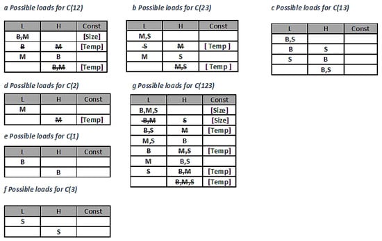
Figure 2.
Possible loads for three-shipper example.
Many versions are possible depending on the stopping conditions. We try two; I requires stopping after just one guess if technical feasibility results, corresponding to a rapid loader that does not want to try to choose again to lower cost, and does not care about rejecting shippers. In II the loader picks again without replacement, to try to lower the cost with a workable or stable choice. One could set the stopping criterion to up to four attempts, since there are at most four possibilities (for ); any more would not be useful. For version I, there are 64 potential feasible outcomes for all coalitions; for II, there is only one outcome possible for each subset.
The loader executes the heuristic on each set in turn as in Table 3 starting at the first level. In I at any particular set one feasible choice is allowed. If a physical constraint is violated, the loader must make another random selection for that set. In II, she continues selecting and checking until the constraint is met and cost is lowered, or the stopping criterion is reached, trying to find a feasible stable solution with lower cost. If the stopping criterion is reached with no feasible outcome, the load cannot be completed by the heuristic, and a different set of packages would be selected for new run of the entire process. Note that random selection with stopping short means that for a larger set of shippers, even though there actually could be a legitimate choice, the algorithm may not find it, and declares impossibility. This can happen with advanced heuristics with complex calculation techniques, if randomness is present. Hopefully the heuristic designer builds in some checks to prevent that; here inspection suffices.
The stable solution found by the process is not necessarily the lowest cost solution, or the cheapest stable solution. A more intelligent heuristic could find a better one. This could be a long process for a large number of shippers; worst case, it is no improvement over an enumeration.
6.4. Outcomes
Table 4 gives the possible costs for each subset, and outcomes for two runs of I (bolded) and one of II (italicized). Using I, there are 64 possible random selections of feasible subset costs. Each run of I resulted in identical selections for all but the entire set. At the final stage of loading all three packages, if the loader selects the load in the fourth row of in Table 4, the cost of 250 is workable but not stable, since 250 exceeds . A second try, selecting the sixth row yields 229, results in a stable loading. The run with II had enough trials to find the minimum cost for every subset; these turned out to be feasible and stable.
Table 4.
Three runs of the example using random FFRO executions I (twice) and II. The load using I (bolded) with final step cost of 229 is stable, but the same with final cost 250 is not. II (italicized) finds the lowest cost stable solution with certainty when stopping criterion allows four trials (to make sure the low cost for is found). For each choice NF = not feasible; -Z (size), -T (temperature) signifies reason for infeasibility. (w) = workable; (s) = stable. All doubletons are workable.
While the algorithm does not include calculating a core allocation, we could append a calculation of the nucleolus. In the case of three shippers, there is a closed form using the five step procedure of []. The nucleolus of the stable game from I with cost of 229 is (125, 62, 42) for (B, M, S); only one of the five cases from [] is relevant in any game with a core. A diagram of the core for three-player games can be made in a triangle plot, as in Figure 3, in which we also plotted the nucleolus, more or less central.
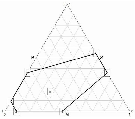
Figure 3.
Plot of the core of the stable result of I in triangular coordinates, with nucleolus n shown. Source: author.
One expects [,] that if there is too little fixed cost to divide, it will no longer be economical for shippers to join together for loading. The same setup with can be used to produce a game that is not even workable. This can be done by selecting randomly the cheapest load option for every subset and the costliest option for the entire set.
7. Conclusions
The MCV loading problem is increasingly important because it provides a way to consolidate units requiring different conditions into one vehicle to lower cost—both shippers and carriers want this. Consolidators also face the problem of quoting a charge to different shippers when the cost estimate is sensitive to the exact loading pattern. The problem is NP hard and must be calculated via heuristic; many such routines are being published as the problem becomes more relevant to today’s logistics, particularly so-called ’last mile’ transport, a particular issue for cold chain and perishable items. Resulting cost estimates and loading plans are very seldom optimal. However, the cost must still be divided.
Here we propose a new technique for setting up such a problem, which uses the chosen heuristic inductively to find the costs of each possible subset of shippers, simultaneously constructing constraints on the cost estimate so that the resulting costs selected are also stable. There is then a guaranteed way (the nucleolus) to divide the total cost among the shippers in a fair manner. Most of the literature on the MCV ignores the question of fair cost allocation, concentrating on finding efficient heuristics for different specialized variants.
Our position is that the two problems are inherently interconnected in the real world. The induction mechanism proposed combines nicely with Peleg’s [] induction scheme for creating minimal balanced collections to generate just the right constraints on the costs obtained to assure the entire cooperative game has a core. We do not claim that the core allocation suggested, the nucleolus, is explainable to the shippers, but the method guarantees that it will be fair.
We have left out the VR problem in our optimization discussion. Our target is method description rather than a complete solution technique, so we focus only on the MCV part of the problem. If the units shipped have the same destination, the order packed may affect cost of the routing, and also needs to be divided. Capturing the routing cost based on loading sequence could be modeled in the heuristic. If there are different destinations, the VR problem must be combined with the MCV because the cost will vary with the order loaded and the routing adopted, which is a different decision problem. Further research could apply our paradigm to the problem to arrive at a stable cost for the combination of load and route.
Another interesting area for research is to utilize recent work on characterization sets for the nucleolus (for instance [,]) to restrict further the number of constraints that need to be tested at each step. This would improve the speed of the approach as well as possibly building the solution calculation into the algorithm. Such a combined process could increase the utility of the method; becoming an AI-like integrated approach to estimating and sharing the cost. This might have more appeal for consolidators and shippers alike. Smart contracts could be developed using such a scheme that would assure all that the shippers would be getting charged an amount which they could not improve on by leaving the group. The issue of explanation would no longer have the thrust it had when people needed to explain. It could be done once and hold for any contract using the technique.
Of course we encourage more work on heuristics and constraint construction for the many practical implementations arising in the world of logistics today. The problem has a fascination and a real business impact that increases in importance.
Conflicts of Interest
The author declares no conflict of interest.
References
- Qin, H.; Zhang, Z.; Qi, Z.; Lim, A. The freight consolidation and containerization problem. Eur. J. Oper. Res. 2014, 234, 37–48. [Google Scholar] [CrossRef]
- Mesa-Arango, R.; Ukkusuri, S. Benefits of in-vehicle consolidation in less than truckload freight transportation operations. Transp. Res. Part E Logist. Transp. Rev. 2013, 60, 113–125. [Google Scholar] [CrossRef]
- Lennane, A. IATA to review air cargo load factor calculations after Project Selfie revelations. Loadstar 2018. Available online: https://theloadstar.co.uk/iata-review-air-cargo-load-factor-calculations-project-selfie-revelations (accessed on 18 January 2018).
- Ramos, A.; Oliveira, J.; Goncalves, J.; Lopes, M. A container loading algorithm with static mechanical equilibrium stability constraints. Transp. Res. B 2016, 91, 565–581. [Google Scholar] [CrossRef]
- Dror, M.; Hartman, B. Shipment consolidation—Who pays for it and how much. Manag. Sci. 2006, 3, 78–87. [Google Scholar] [CrossRef]
- Alonso, M.T.; Alvarez-Valdes, R.; Iori, M.; Parreño, F.; Tamarit, J.M. Mathematical models for multicontainer loading problems. Omega 2016. [Google Scholar] [CrossRef]
- Gonçalves, J.F.; Resende, M.G.C. A parallel multi-population biased random-key genetic algorithm for a container loading problem. Comput. Oper. Res. 2012, 39, 179–190. [Google Scholar] [CrossRef]
- Alvarez-Valdes, R.; Parreño, F.; Tamarit, J.M. A GRASP/Path Relinking Algorithm for two- and three-dimensional multiple bin-size packing problems. Comput. Oper. Res. 2013, 40, 3081–3090. [Google Scholar] [CrossRef]
- Pollaris, H.; Braekers, K.; Janssens, A.C.; Janssens, G.; Limbourg, S. Iterated Local Search for the Capacitated Vehicle Routing Problem with Sequence Based Pallet Loading and Axle Weight Constraints. Networks 2017, 69, 304–316. [Google Scholar] [CrossRef]
- Junquiera, L.; Morabito, R.; Yamashita, D.S. Three-dimensional container loading models with cargo stability and load bearing constraints. Comput. Oper. Res. 2012, 39, 74–85. [Google Scholar] [CrossRef]
- Peleg, B. An Inductive method for constructing minimal balanced collections of finite sets. Nav. Res. Logist. 1965, 12, 155–162. [Google Scholar] [CrossRef]
- Young, H.P. Cost Allocation: Methods, Principles, Applications; Elsevier Science Publishers B.V.: Amsterdam, The Netherlands, 1985. [Google Scholar]
- Peleg, B.; Sudhölter, P. Introduction to the Theory of Cooperative Games; Springer: Berlin, Germany, 2007. [Google Scholar]
- Dror, M.; Hartman, B.; Chang, W. The Cost Allocation Issue in Joint Replenishment. Int. J. Prod. Econ. 2011, 136, 232–244. [Google Scholar] [CrossRef]
- Schmeidler, D. Nucleolus of a characteristic function game. SIAM J. Appl. Math. 1969, 17, 1163–1170. [Google Scholar] [CrossRef]
- Hartman, B.; Dror, M. Cost allocation in continuous-review inventory models. Nav. Res. Logist. 1996, 43, 549–561. [Google Scholar] [CrossRef]
- Anshelevich, E.; Dasgupta, A.; Kleinburg, J.; Tardos, E.; Wexler, T.; Roughgarden, T. The price of stability for network design with fair cost allocation. SIAM J. Comput. 2008, 38, 1602–1623. [Google Scholar] [CrossRef]
- Moulin, H.; Shenker, S. Strategyproof sharing of submodular costs: Budget balance versus efficiency. Econ. Theory 2001, 18, 511–513. [Google Scholar] [CrossRef]
- Perry, J.; Zentz, C. FERC Rejects SPP’s Cost Allocation Plan for Two Interregional Transmission Projects. Lexology 2017. Available online: https://www.lexology.com/library/detail.aspx?g=38231f1c-b986-41c0-8bf1-982a85da6e13 (accessed on 10 March 2018).
- Guajardo, M.; Rönnquist, M. A review on cost allocation methods in collaborative transportation. Int. Trans. Oper. Res. 2016, 3, 371–392. [Google Scholar] [CrossRef]
- Fang, X.; Cho, S.-H. Stability and endogenous formation of inventory transshipment networks. Oper. Res. 2014, 62, 1316–1334. [Google Scholar] [CrossRef]
- Bondareva, O. Theory of the core in the n-person game. Vestnik LGU 1962, 13, 141–142. [Google Scholar]
- Shapley, L. On balanced sets and cores. Nav. Res. Logist. 1967, 14, 453–460. [Google Scholar] [CrossRef]
- Solymosi, T.; Sziklai, B. Characterization Sets for the Nucleolus in Balanced Games. Oper. Res. Lett. 2016, 44, 520–524. [Google Scholar] [CrossRef]
- Solymosi, T.; Sziklai, B. Universal Characterization Sets for the Nucleolus in Balanced Games; Discussion Paper MT-DP-2015/12; Centre for Economic and Regional Studies, Hungarian Academy of Sciences: Budapest, Hungary, 2015. [Google Scholar]
- Puerto, J.; Perea, F. Finding the nucleolus of any n-person cooperative game by a single linear program. Comput. Oper. Res. 2013, 40, 2308–2313. [Google Scholar] [CrossRef]
- Leng, M.; Parlar, M. Analytic Solution for the Nucleolus of a Three-Player Cooperative Game. Nav. Res. Logist. 2010, 57, 667–672. [Google Scholar] [CrossRef]
© 2018 by the author. Licensee MDPI, Basel, Switzerland. This article is an open access article distributed under the terms and conditions of the Creative Commons Attribution (CC BY) license (http://creativecommons.org/licenses/by/4.0/).