A Complete Analysis on the Risk of Using Quantal Response: When Attacker Maliciously Changes Behavior under Uncertainty

Abstract

In security games, the defender often has to predict the attacker’s behavior based on some observed attack data. However, a clever attacker can intentionally change its behavior to mislead the defender’s learning, leading to an ineffective defense strategy. This paper investigates the attacker’s imitative behavior deception under uncertainty, in which the attacker mimics a (deceptive) Quantal Response behavior model by consistently playing according to a certain parameter value of that model, given that it is uncertain about the defender’s actual learning outcome. We have three main contributions. First, we introduce a new maximin-based algorithm to compute a robust attacker deception decision under uncertainty, given the defender is unaware of the attacker deception. Our polynomial algorithm is built via characterizing the decomposability of the attacker deception space as well optimal deception behavior of the attacker against the worst case of uncertainty. Second, we propose a new counter-deception algorithm to tackle the attacker’s deception. We theoretically show that there is a universal optimal defense solution, regardless of any private knowledge the defender has about the relation between their learning outcome and the attacker deception choice. Third, we conduct extensive experiments in various security game settings, demonstrating the effectiveness of our proposed counter-deception algorithms to handle the attacker manipulation.

1. Introduction

In many real-world security domains, security agencies (defender) attempt to predict the attacker’s future behavior based on some collected attack data, and use the prediction result to determine effective defense strategies. A lot of existing work in security games has thus focused on developing different behavior models of the attacker [1,2,3]. Recently, the challenge of playing against a deceptive attacker has been studied, in which the attacker can manipulate the attack data (by changing its behavior) to fool the defender, making the defender learn a wrong behavior model of the attacker [4]. Such deceptive behavior by the attacker can lead to an ineffective defender strategy.

A key limitation in existing work is the assumption that the defender has full access to the attack data, which means the attacker knows exactly what the learning outcome of the defender would be. However, in many real-world domains, the defender often has limited access to the attack data, e.g., in wildlife protection, park rangers typically cannot find all the snares laid out by poachers in entire conservation areas [5]. As a result, the learning outcome the defender obtains (with limited attack data) may be different from the deception behavior model that the attacker commits to. Furthermore, the attacker (and the defender) may have imperfect knowledge about the relation between the deception choice of the attacker and the actual learning outcome of the defender.

We address this limitation by studying the challenge of attacker deception given such uncertainty. We consider a security game model in which the defender adopts Quantal Response ($\mathtt{QR}$), a well-known behavior model in economics and game theory [2,6,7], to predict the attacker’s behavior, where the model parameter $\lambda \in \mathbb{R}$ is trained based on some attack data. On the other hand, the attacker plays deceptively by mimicking a $\mathtt{QR}$ model with a different value of $\lambda$, denoted by ${\lambda }^{\mathrm{dec}}$. In this work, we incorporate the deception-learning uncertainty into this game model, where the learning outcome of the defender (denoted by ${\lambda }^{\mathrm{learnt}}$) can be any value within a range centered at ${\lambda }^{\mathrm{dec}}$.

We provide the following key contributions. First, we present a new maximin-based algorithm to compute an optimal robust deception strategy for the attacker. At a high level, our algorithm works by maximizing the attacker’s utility under the worst-case of uncertainty. The problem comprises of three nested optimization levels, which is not straightforward to solve. We thus propose an alternative single-level optimization problem based on partial discretization. Despite this simplification, the resulting optimization is still challenging to solve due to the non-convexity of the attacker’s utility and the dependence of the uncertainty set on ${\lambda }^{\mathrm{dec}}$. By exploiting the decomposibility of the deception space and the monotonicity of the attacker’s utility, we show that the alternative relaxed problem can be solved optimally in polynomial time. The idea is to decompose the problem into a polynomial number of sub-problems (according to the decomposition of the deception space)—each sub problem can be solved in a polynomial time given the attacker optimal deception decision within each sub-space is shown to be one of the extreme points of that sub-space, despite the non-convexity of the sub-problem.

Second, we propose a new counter-deception algorithm, which generates an optimal defense function that outputs a defense strategy for each possible (deceptive) learning outcome. Our key finding is that there is a universal optimal defense function for the defender, regardless of any additional information he has about the relation between their learning outcome and the deception choice of the attacker (besides the common knowledge that the learning outcome is within a range around the deception choice). Importantly, this optimal defense function, which can be determined by solving a single non-linear program, only outputs two different strategies despite the infinite-sized learning outcome space. Our counter-deception algorithm is built based on an extensive in-depth analysis of intrinsic characteristics of the attacker’s adaptive deception response to any deception-aware defense solution. That is, under our propose defense mechanism, the attacker’s deception space remains decomposable (although the sub-spaces vary which depends on the counter-deception mechanism) and the attacker’s optimal deception remains one of the extreme points of the deception sub-spaces.

Third, we conduct extensive experiments to evaluate our proposed algorithms in various security game settings with different number of targets, various ranges of the defender capacity as well as different levels of the attacker uncertainty, and finally, different correlations between players’ payoffs. Our results show that (i) despite the uncertainty, the attacker still obtains a significantly higher utility by playing deceptively when the defender is unaware of the attacker deception; and (ii) the defender can substantially diminish the impact of the attacker’s deception when following our counter-deception algorithm.

Outline of the Article

We outline the rest of our article as follows. We discuss the Related Work and Background in Section 2 and Section 3. In Section 4, we present our detailed theoretical analysis on the attacker behavior deception under the uncertainty of the defender’s learning outcome, given that the defender is unaware of the attacker’s deception. In Section 5, we describe our new counter-deception algorithm for the defender to tackle the attacker’s manipulation. In this section, we first extend theoretical results in Section 4 as to analyzing the attacker manipulation adaptation to the defender’s counter-deception. Based on the result of the attacker adaptation, we then provide theoretical results on computing the defender optimal counter-deception. In Section 6, we show our experiment results, evaluating our proposed algorithms. Finally, Section 7 concludes our article.

2. Related Work

Parameterized models of attacker behavior such as Quantal Response, and other machine learning models have been studied for Stackelberg security games ($\mathtt{SSG}$s) [5,8,9]. These models provide general techniques for modeling the attacker decision making. Prior work assumes that the attacker always plays truthfully. Thus, existing algorithms for generating defense strategies would be vulnerable against deceptive attacks by an attacker who is aware of the defender’s learning. Our work addresses such a strategic deceptive attacker by planning counter-deception defense strategies.

Deception is widely studied in security research [10,11,12,13,14,15]. In $\mathtt{SSG}$ literature, a lot of prior work has studied deception by the defender, i.e., the defender exploits their knowledge regarding uncertainties to mislead the attacker’s decision making [16,17,18,19]. Recently, deception on the attacker’s side has been studied. Existing work focuses on situations in which the defender is uncertain about the attacker type [20,21,22]. Some study the attacker behavior deception problem [4,23]. They assume that the attacker knows exactly the learning outcome while in our problem, the attacker is uncertain about that learning outcome.

Our work is also related to poisoning attacks in adversarial machine learning in which an adversary can contaminate the training data to mislead ML algorithms [24,25,26,27]. Existing work in adversarial learning uses prediction accuracy as the measure to analyzing such attacks, while in our game setting, the final goals of players are to optimize their utility, given some learning outcome.

3. Background

Stackelberg Security Games ($\mathtt{SSG}$s). There is a set of $\mathbf{T}=\{1,2,\cdots ,T\}$ targets that a defender has to protect using $L<T$ security resources. A pure strategy of the defender is an allocation of these L resources over the T targets. A mixed strategy of the defender is a probability distribution over all pure strategies. In this work, we consider the no-scheduling-constraint game setting, in which each defender mixed strategy can be compactly represented as a coverage vector $\mathbf{x}=\{x_1,x_2,\cdots ,x_T\}$, where $x_t\in [0,1]$ is the probability that the defender protects target t and ${\sum }_t{x}_t\le L$ [28]. We denote by $\mathbf{X}$ the set of all defense strategies. In $\mathtt{SSG}$s, the defender plays first by committing to a mixed strategy, and the attacker responds against this strategy by choosing a single target to attack.

When the attacker attacks target t, it obtains a reward $R_t^a$ while the defender receives a penalty $P_t^d$ if the defender is not protecting that target. Conversely, if the defender is protecting t, the attacker gets a penalty $P_t^a<R_t^a$ while the defender receives a reward $R_t^d>P_t^d$. The expected utility of the defender, $U_t^d\left(x_t\right)$ (and attacker’s, $U_t^a\left(x_t\right)$), if the attacker attacks target t are computed as follows:

$$U_t^d\left(x_t\right)=x_t{R}_t^d+(1-x_t)P_t^d{U}_t^a\left(x_t\right)=x_t{P}_t^a+(1-x_t)R_t^a$$

Quantal Response Model ($\mathtt{QR}$).$\mathtt{QR}$ is a well-known behavioral model used to predict boundedly rational (attacker) decision making in security games [2,6,7]. Essentially, $\mathtt{QR}$ predicts the probability that the attacker attacks each target t using the softmax function:

$$\begin{array}{cc}\hfill & q_t(\mathbf{x},\lambda )=\frac{e^{\lambda U_t^a\left(x_t\right)}}{{\sum }_{t^{\prime }}{e}^{\lambda U_{t^{\prime }}^a\left(x_{t^{\prime }}\right)}}\hfill \end{array}$$

(1)

where $\lambda$ is the parameter that governs the attacker’s rationality. When $\lambda =0$, the attacker attacks every target uniformly at random. When $\lambda =+\infty$, the attacker is perfectly rational. Given that the attacker follows $\mathtt{QR}$, the defender and attacker’s expected utility is computed as an expectation over all targets:

$$\begin{array}{cc}\hfill & U^d(\mathbf{x},\lambda )={\sum }_t{q}_t(\mathbf{x},\lambda )U_t^d\left(x_t\right)\hfill \end{array}$$

(2)

$$\begin{array}{cc}\hfill & U^a(\mathbf{x},\lambda )={\sum }_t{q}_t(\mathbf{x},\lambda )U_t^a\left(x_t\right)\hfill \end{array}$$

(3)

The attacker’s utility $U^a(\mathbf{x},\lambda )$ was proved to be increasing in $\lambda$ [4]. We leverage this monotonicity property to analyze the attacker’s deception. In $\mathtt{SSG}$s, the defender can learn $\lambda$ based on some collected attack data, denoted by ${\lambda }^{\mathrm{learnt}}$, and find an optimal strategy which maximizes their expected utility accordingly:

$$\begin{array}{c}\hfill \underset{\mathbf{x}\in \mathbf{X}}{max}{U}^d(\mathbf{x},{\lambda }^{\mathrm{learnt}})\end{array}$$

4. Attacker Behavior Deception under Unknown Learning Outcome

We first study the problem of imitative behavior deception in a security scenario in which the attacker does not know exactly the defender’s learning outcome. Formally, if the attacker plays according to a particular parameter value of $\mathtt{QR}$, denoted by ${\lambda }^{\mathrm{dec}}$, the learning outcome of the defender can be any value within the interval $[max\{{\lambda }^{\mathrm{dec}}-\delta ,0\},{\lambda }^{\mathrm{dec}}+\delta ]$, where $\delta >0$ represents the extent to which the attacker is uncertain about the learning outcome of the defender. We term this interval, $[max\{{\lambda }^{\mathrm{dec}}-\delta ,0\},{\lambda }^{\mathrm{dec}}+\delta ]$, as the uncertainty range of ${\lambda }^{\mathrm{dec}}$. We are particularly interested in the research question:

Given uncertainty about learning outcomes of the defender, can the attacker still benefit from playing deceptively?

In this section, we consider the scenario when the attacker plays deceptively while the defender does not take into account the prospect of the attacker’s deception. We aim at analyzing the attacker deception decision in this no-counter-deception scenario. We assume that the attacker plays deceptively by mimicking any ${\lambda }^{\mathrm{dec}}$ within the range $[0,{\lambda }^{max}]$. We consider $\lambda \ge 0$ as this is the widely accepted range of the attacker’s bounded rationality in the literature. The value ${\lambda }^{max}$ represents the limit to which the attacker plays deceptively. When ${\lambda }^{max}\to \infty$, the deception range of the attacker covers the whole range of $\lambda$. We aim at examining the impact of ${\lambda }^{max}$ on the deception outcome of the attacker later in our experiments. Given uncertainty about the learning outcome of the defender, the attacker attempts to find the optimal ${\lambda }^{\mathrm{dec}}\in [0,{\lambda }^{max}]$ to imitate that maximizes its utility in the worst case scenario of uncertainty, which can be formulated as follows:

$$\begin{array}{cc}\hfill \left({\mathbf{P}}^{\mathrm{dec}}\right):\underset{{\lambda }^{\mathrm{dec}}}{max}\underset{{\lambda }^{\mathrm{learnt}}}{min}& U^a(\mathbf{x}\left({\lambda }^{\mathrm{learnt}}\right),{\lambda }^{\mathrm{dec}})\hfill \\ \hfill \mathrm{s}.\mathrm{t}.& {\lambda }^{\mathrm{dec}}\in [0,{\lambda }^{max}]\hfill \\ \hfill & max\{{\lambda }^{\mathrm{dec}}-\delta ,0\}\le {\lambda }^{\mathrm{learnt}}\le {\lambda }^{\mathrm{dec}}+\delta \hfill \\ \hfill & \mathbf{x}\left({\lambda }^{\mathrm{learnt}}\right)\in \underset{{\mathbf{x}}^{\prime }\in \mathbf{X}}{argmax}{U}^d({\mathbf{x}}^{\prime },{\lambda }^{\mathrm{learnt}})\hfill \end{array}$$

where $\mathbf{x}\left({\lambda }^{\mathrm{learnt}}\right)$ is the defender’s optimal strategy w.r.t their learning outcome ${\lambda }^{\mathrm{learnt}}$. The objective $U^a(\mathbf{x}\left({\lambda }^{\mathrm{learnt}}\right),{\lambda }^{\mathrm{dec}})$ is the attacker’s utility when the defender plays $\mathbf{x}\left({\lambda }^{\mathrm{learnt}}\right)$ and the attacker mimics $\mathtt{QR}$ with ${\lambda }^{\mathrm{dec}}$ to play (see Equations (1)–(3) for the detailed computation). In addition, $U^d({\mathbf{x}}^{\prime },{\lambda }^{\mathrm{learnt}})$ is the defender’s expected utility that the defender aims to maximize where ${\mathbf{x}}^{\prime }$ is the defender’s strategy and ${\lambda }^{\mathrm{learnt}}$ is the learning outcome of the defender regarding the attacker’s behavior. Essentially, the last constraint of $\left({\mathbf{P}}^{\mathrm{dec}}\right)$ ensures that the defender will play an optimal defense strategy according to their learning outcome. Finally, due to potential noises in learning, the defender’s learning outcome ${\lambda }^{\mathrm{learnt}}$ may fall outside of the deception range of the attacker, which is captured by our constraint that ${\lambda }^{\mathrm{learnt}}\le {\lambda }^{\mathrm{dec}}+\delta$.

4.1. A Polynomial-Time Deception Algorithm

The optimization problem $\left({\mathbf{P}}^{\mathrm{dec}}\right)$ involves three-nested optimization levels which is not straightforward to solve. We thus propose to limit the possible learning outcomes of the defender by discretizing the domain of ${\lambda }^{\mathrm{learnt}}$ into a finite set ${\mathsf{\Lambda }}_{\mathrm{discrete}}^{\mathrm{learnt}}=({\lambda }_1^{\mathrm{learnt}},{\lambda }_2^{\mathrm{learnt}},\dots ,{\lambda }_K^{\mathrm{learnt}})$ where ${\lambda }_1^{\mathrm{learnt}}=0$, ${\lambda }_K^{\mathrm{learnt}}={\lambda }^{max}+\delta$, and ${\lambda }_{k+1}^{\mathrm{learnt}}-{\lambda }_k^{\mathrm{learnt}}=\eta ,\forall k<K$ where $\eta >0$ is the discretization step size and $K=\frac{{\lambda }^{max}+\delta }{\eta }+1$ is the number of discrete learning values1. For each deception choice ${\lambda }^{\mathrm{dec}}$, the attacker’s uncertainty set of defender’s possible learning outcomes ${\lambda }^{\mathrm{learnt}}$ is now given by:

$$\begin{array}{cc}\hfill & {\mathsf{\Lambda }}_{\mathrm{discrete}}^{\mathrm{learnt}}\left({\lambda }^{\mathrm{dec}}\right)={\mathsf{\Lambda }}_{\mathrm{discrete}}^{\mathrm{learnt}}\cap [{\lambda }^{\mathrm{dec}}-\delta ,{\lambda }^{\mathrm{dec}}+\delta ]\hfill \end{array}$$

For each ${\lambda }_k^{\mathrm{learnt}}$, we can easily compute the corresponding optimal defense strategy $\mathbf{x}\left({\lambda }_k^{\mathrm{learnt}}\right)$ in advance [2]. We thus obtain a simplified optimization problem:

$$\begin{array}{cc}\hfill \left({\mathbf{P}}_{\mathrm{discrete}}^{\mathrm{dec}}\right):& \underset{{\lambda }^{\mathrm{dec}}\in [0,{\lambda }^{max}]}{max}U\hfill \\ \hfill & \mathrm{s}.\mathrm{t}.U\le U^a(\mathbf{x}\left({\lambda }_k^{\mathrm{learnt}}\right),{\lambda }^{\mathrm{dec}}),\mathrm{for}\mathrm{all}{\lambda }_k^{\mathrm{learnt}}\in {\mathsf{\Lambda }}_{\mathrm{discrete}}^{\mathrm{learnt}}\left({\lambda }^{\mathrm{dec}}\right)\hfill \end{array}$$

where U is the maximin utility for the attacker in the worst-case of learning outcome.

Remark on computational challenge. Although $\left({\mathbf{P}}_{\mathrm{discrete}}^{\mathrm{dec}}\right)$ is a single-level optimization, solving it is still challenging due to (i) $\left({\mathbf{P}}_{\mathrm{discrete}}^{\mathrm{dec}}\right)$ is a non-convex optimization problem since the attacker’s utility $U^a(\mathbf{x}\left({\lambda }_k^{\mathrm{learnt}}\right),{\lambda }^{\mathrm{dec}})$ is non-convex in ${\lambda }^{\mathrm{dec}}$; and (ii) the number of inequality constraints in $\left({\mathbf{P}}_{\mathrm{discrete}}^{\mathrm{dec}}\right)$ vary with respect to ${\lambda }^{\mathrm{dec}}$, which complicates the problem further. By exploiting the decomposability property of the deception space $[0,{\lambda }^{max}]$ and the monotonicity of the attacker’s utility function $U^a(\mathbf{x}\left({\lambda }_k^{\mathrm{learnt}}\right),{\lambda }^{\mathrm{dec}})$, we show that $\left({\mathbf{P}}_{\mathrm{discrete}}^{\mathrm{dec}}\right)$ can be solved optimally in a polynomial time.

Theorem 1

(Time complexity). (${\mathbf{P}}_{\mathit{discrete}}^{\mathit{dec}}$) can be solved optimally in a polynomial time.

Overall, the proof of Theorem 1 is derived based on (i) Lemma 1—showing that the deception space can be divided into an $O\left(K\right)$ number of sub-intervals, and each sub-interval leads to the same uncertainty set; and (ii) Lemma 4—showing that (${\mathbf{P}}_{\mathrm{discrete}}^{\mathrm{dec}}$) can be divided into a $O\left(K\right)$ sub-problems which correspond to the decomposability of the deception space (as shown in Lemma 1), and each sub-problem can be solved in polynomial time.

4.1.1. Decomposability of Deception Space

In the following, we first present our theoretical analysis on the decomposability of the deception space. We then describe in detail our decomposition algorithm.

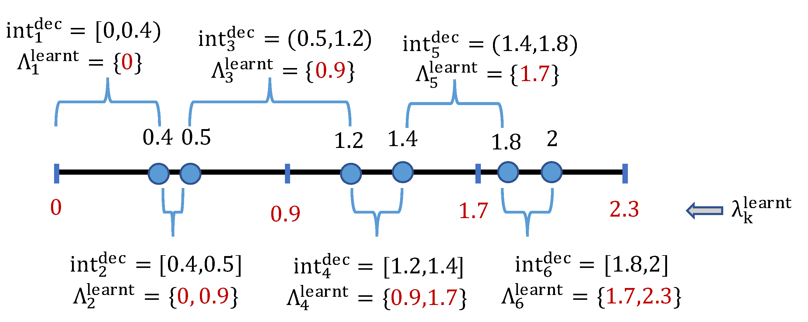
Lemma 1

(Decomposability of deception space). The attacker deception space $[0,{\lambda }^{max}]$ can be decomposed into a finite number of disjointed sub-intervals, denoted by $in{t}_j^{\mathit{dec}}$ where $j=1,2,\cdots ,$ and $in{t}_j^{\mathit{dec}}\cap in{t}_{j^{\prime }}^{\mathit{dec}}=\varnothing$ for all $j\ne j^{\prime }$ and ${\cup }_{j}in{t}_j^{\mathit{dec}}=[0,{\lambda }^{max}]$, such that each ${\lambda }^{\mathit{dec}}\in in{t}_j^{\mathit{dec}}$ leads to the same uncertainty set of learning outcomes, denoted by ${\mathsf{\Lambda }}_j^{\mathit{learnt}}\subseteq {\mathsf{\Lambda }}_{\mathit{discrete}}^{\mathit{learnt}}$. Furthermore, these sub-intervals and uncertainty sets $(in{t}_j^{\mathit{dec}},{\mathsf{\Lambda }}_j^{\mathit{learnt}})$ can be found in a polynomial time.

The proof of Lemma 1 is derived based on Lemmas 2 and 3. An example of the deception-space decomposition is illustrated in Figure 1. Intuitively, although the deception space $[0,{\lambda }^{max}]$ is infinite, the total number of possible learning-outcome uncertainty sets is at most $2^K$ (i.e., the number of subsets of the discrete learning space ${\mathsf{\Lambda }}_{\mathit{discrete}}^{\mathit{learnt}}$). Therefore, the deception space can be divided into a finite number of disjoint subsets such that any deception value ${\lambda }^{\mathit{dec}}$ within each subset will lead to the same uncertainty set. Moreover, each of these deception subsets form a sub-interval of $[0,{\lambda }^{max}]$, which is derived from Lemma 2:

Lemma 2.

Given two deception values ${\lambda }_1^{\mathit{dec}}<{\lambda }_2^{\mathit{dec}}\in [0,{\lambda }^{max}]$, if the learning uncertainty sets corresponding to these two values are the same, i.e., ${\mathsf{\Lambda }}_{\mathit{discrete}}^{\mathit{learnt}}\left({\lambda }_1^{\mathit{dec}}\right)\equiv {\mathsf{\Lambda }}_{\mathit{discrete}}^{\mathit{learnt}}\left({\lambda }_2^{\mathit{dec}}\right)$, then for any deception value ${\lambda }_1^{\mathit{dec}}<{\lambda }^{\mathit{dec}}<{\lambda }_2^{\mathit{dec}}$, its uncertainty set is also the same, that is:

$$\begin{array}{c}\hfill {\mathsf{\Lambda }}_{\mathrm{discrete}}^{\mathrm{learnt}}\left({\lambda }^{\mathrm{dec}}\right)\equiv {\mathsf{\Lambda }}_{\mathrm{discrete}}^{\mathrm{learnt}}\left({\lambda }_1^{\mathrm{dec}}\right)\equiv {\mathsf{\Lambda }}_{\mathrm{discrete}}^{\mathrm{learnt}}\left({\lambda }_2^{\mathrm{dec}}\right)\end{array}$$

The remaining analysis for Lemma 1 is to show that these deception sub-intervals can be found in polynomial time, which is obtained based on Lemma 3:

Lemma 3.

For each learning outcome ${\lambda }_k^{\mathit{learnt}}$, there are at most two deception sub-intervals such that ${\lambda }_k^{\mathit{learnt}}$ is the smallest learning outcome in the corresponding learning uncertainty set. As a result, the total number of deception sub-intervals is $O\left(K\right)$, which is polynomial.

Since there is a $O\left(K\right)$ number of deception sub-intervals, we now can develop a polynomial-time algorithm (Algorithm 1) which iteratively divides the deceptive range $[0,{\lambda }^{max}]$ into multiple intervals, denoted by ${\left\{in{t}_j^{\mathrm{dec}}\right\}}_j$. Each of these intervals, $in{t}_j^{\mathrm{dec}}$, corresponds to the same uncertainty set of possible learning outcomes for the defender, denoted by ${\mathsf{\Lambda }}_j^{\mathrm{learnt}}$.

In this algorithm, for each ${\lambda }_k^{\mathrm{learnt}}$, we denote by $l{b}_k={\lambda }_k^{\mathrm{learnt}}-\delta$ and $u{b}_k={\lambda }_k^{\mathrm{learnt}}+\delta$ the smallest and largest possible values of ${\lambda }^{\mathrm{dec}}$ so that ${\lambda }_k^{\mathrm{learnt}}$ belongs to the uncertainty set of ${\lambda }^{\mathrm{dec}}$. In Algorithm 1, $start$ is the variable which represents the left bound of each interval $in{t}_j^{\mathrm{dec}}$. The variable $open$ indicates if $in{t}_j^{\mathrm{dec}}$ is left-open ($open=true$) or not ($open=false$). If $start$ is known for $in{t}_j^{\mathrm{dec}}$, the uncertainty set ${\mathsf{\Lambda }}_j^{\mathrm{learnt}}$ can be determined as follows:

$$\begin{array}{cc}\hfill & {\mathsf{\Lambda }}_j^{\mathrm{learnt}}=\{{\lambda }_k^{\mathrm{learnt}}:{\lambda }_k^{\mathrm{learnt}}\in [start-\delta ,start+\delta ]\}\mathrm{if}in{t}_j^{\mathrm{dec}}\mathrm{is}\mathrm{left}-\mathrm{closed}\hfill \\ \hfill & {\mathsf{\Lambda }}_j^{\mathrm{learnt}}=\{{\lambda }_k^{\mathrm{learnt}}:{\lambda }_k^{\mathrm{learnt}}\in (start-\delta ,start+\delta ]\}\mathrm{if}in{t}_j^{\mathrm{dec}}\mathrm{is}\mathrm{left}-\mathrm{open}\hfill \end{array}$$

Initially, $start$ is set to 0 which is the lowest possible value of ${\lambda }^{\mathrm{dec}}$ such that the uncertainty range $[{\lambda }^{\mathrm{dec}}-\delta ,{\lambda }^{\mathrm{dec}}+\delta ]$ contains ${\lambda }_1^{\mathrm{learnt}}$ and $open=false$. Given $start$ and its uncertainty range $[start-\delta ,start+\delta ]$, the first interval $in{t}_1^{\mathrm{dec}}$ of ${\lambda }^{\mathrm{dec}}$ corresponds to the uncertainty set determined as follows:

$$\begin{array}{cc}\hfill & {\mathsf{\Lambda }}_1^{\mathrm{learnt}}=\{{\lambda }_k^{\mathrm{learnt}}\in {\mathsf{\Lambda }}^{\mathrm{learnt}}:{\lambda }_k^{\mathrm{learnt}}\in [start-\delta ,start+\delta ]\}\hfill \end{array}$$

At each iteration j, given the left bound $start$ and the uncertainty set ${\mathsf{\Lambda }}_j^{\mathrm{learnt}}$ of the interval $in{t}_j^{\mathrm{dec}}$, Algorithm 1 determines the right bound of $in{t}_j^{\mathrm{dec}}$, the left bound of the next interval $in{t}_{j+1}^{\mathrm{dec}}$ (by updating $start$), and the uncertainty set ${\mathsf{\Lambda }}_{j+1}^{\mathrm{learnt}}$, (lines (6–15)). Finally, we prove the correctness of Algorithm 1 by presenting Proposition 1, which shows that for any ${\lambda }^{\mathrm{dec}}$ within each interval $in{t}_j^{\mathrm{dec}}$, the corresponding uncertainty interval $[{\lambda }^{\mathrm{dec}}-\delta ,{\lambda }^{\mathrm{dec}}+\delta ]$ covers the same uncertainty set ${\mathsf{\Lambda }}_j^{\mathrm{learnt}}$.

Algorithm 1: Imitative behavior deception—Decomposition of QR parameter domain into sub-intervals

Proposition 1

(Correctness of Algorithm 1). Each iteration j of Algorithm 1 returns an interval $in{t}_j^{\mathit{dec}}$ such that each ${\lambda }^{\mathit{dec}}\in in{t}_j^{\mathit{dec}}$ leads to the same uncertainty set:

$$\begin{array}{cc}\hfill & {\mathsf{\Lambda }}_j^{\mathit{learnt}}=\{{\lambda }_{k_j^{min}}^{\mathit{learnt}},\dots ,{\lambda }_{k_j^{max}}^{\mathit{learnt}}\}\hfill \end{array}$$

The rest of this section will provide details of missing proofs for the aforementioned theoretical results.

Proof of Lemma 2.

For any ${\lambda }^{\mathrm{learnt}}\in {\mathsf{\Lambda }}_{\mathrm{discrete}}^{\mathrm{learnt}}\left({\lambda }_1^{\mathrm{dec}}\right)\equiv {\mathsf{\Lambda }}_{\mathrm{discrete}}^{\mathrm{learnt}}\left({\lambda }_2^{\mathrm{dec}}\right)$, we have:

$$\begin{array}{cc}\hfill & {\lambda }_1^{\mathrm{dec}}-\delta \le {\lambda }^{\mathrm{learnt}}\le {\lambda }_1^{\mathrm{dec}}+\delta \hfill \\ \hfill & {\lambda }_2^{\mathrm{dec}}-\delta \le {\lambda }^{\mathrm{learnt}}\le {\lambda }_2^{\mathrm{dec}}+\delta \hfill \end{array}$$

Since ${\lambda }^{\mathrm{dec}}\in ({\lambda }_1^{\mathrm{dec}},{\lambda }_2^{\mathrm{dec}})$, we obtain:

$$\begin{array}{cc}\hfill & {\lambda }^{\mathrm{dec}}-\delta \le {\lambda }^{\mathrm{learnt}}\le {\lambda }^{\mathrm{dec}}+\delta \hfill \end{array}$$

which implies ${\lambda }^{\mathrm{learnt}}\in {\mathsf{\Lambda }}_{\mathrm{discrete}}^{\mathrm{learnt}}\left({\lambda }^{\mathrm{dec}}\right)$. As a result,

$$\begin{array}{ccc}\hfill & {\mathsf{\Lambda }}_{\mathrm{discrete}}^{\mathrm{learnt}}\left({\lambda }_1^{\mathrm{dec}}\right)\equiv {\mathsf{\Lambda }}_{\mathrm{discrete}}^{\mathrm{learnt}}\left({\lambda }_2^{\mathrm{dec}}\right)\subseteq {\mathsf{\Lambda }}_{\mathrm{discrete}}^{\mathrm{learnt}}\left({\lambda }^{\mathrm{dec}}\right)\hfill & \hfill (*)\end{array}$$

On the other hand, let us consider a ${\lambda }^{\mathrm{learnt}}\in {\mathsf{\Lambda }}_{\mathrm{discrete}}^{\mathrm{learnt}}\left({\lambda }^{\mathrm{dec}}\right)$, or equivalently, ${\lambda }^{\mathrm{dec}}-\delta \le {\lambda }^{\mathrm{learnt}}\le {\lambda }^{\mathrm{dec}}+\delta$. We are going to show that this ${\lambda }^{\mathrm{learnt}}\in {\mathsf{\Lambda }}_{\mathrm{discrete}}^{\mathrm{learnt}}\left({\lambda }_1^{\mathrm{dec}}\right)\equiv {\mathsf{\Lambda }}_{\mathrm{discrete}}^{\mathrm{learnt}}\left({\lambda }_2^{\mathrm{dec}}\right)$ as well. Indeed, let us assume ${\lambda }^{\mathrm{learnt}}\notin {\mathsf{\Lambda }}_{\mathrm{discrete}}^{\mathrm{learnt}}\left({\lambda }_1^{\mathrm{dec}}\right)\equiv {\mathsf{\Lambda }}_{\mathrm{discrete}}^{\mathrm{learnt}}\left({\lambda }_2^{\mathrm{dec}}\right)$. It means the following inequalities must hold true:

$$\begin{array}{cc}\hfill & {\lambda }_1^{\mathrm{dec}}+\delta <{\lambda }^{\mathrm{learnt}}<{\lambda }_2^{\mathrm{dec}}-\delta \hfill \end{array}$$

which means that the uncertainty ranges with respect to ${\lambda }_1^{\mathrm{dec}}$ and ${\lambda }_2^{\mathrm{dec}}$ are not overlapped, i.e.,  $[{\lambda }_1^{\mathrm{dec}}-\delta ,{\lambda }_1^{\mathrm{dec}}+\delta ]\cap [{\lambda }_2^{\mathrm{dec}}-\delta ,{\lambda }_2^{\mathrm{dec}}+\delta ]\equiv \varnothing$, or equivalently, ${\mathsf{\Lambda }}_{\mathrm{discrete}}^{\mathrm{learnt}}\left({\lambda }_1^{\mathrm{dec}}\right)\cap {\mathsf{\Lambda }}_{\mathrm{discrete}}^{\mathrm{learnt}}\left({\lambda }_2^{\mathrm{dec}}\right)\equiv \varnothing$, which is contradictory.

Therefore, ${\lambda }^{\mathrm{learnt}}\in {\mathsf{\Lambda }}_{\mathrm{discrete}}^{\mathrm{learnt}}\left({\lambda }_1^{\mathrm{dec}}\right)\equiv {\mathsf{\Lambda }}_{\mathrm{discrete}}^{\mathrm{learnt}}\left({\lambda }_2^{\mathrm{dec}}\right)$, meaning that:

$$\begin{array}{ccc}\hfill & {\mathsf{\Lambda }}_{\mathrm{discrete}}^{\mathrm{learnt}}\left({\lambda }^{\mathrm{dec}}\right)\subseteq {\mathsf{\Lambda }}_{\mathrm{discrete}}^{\mathrm{learnt}}\left({\lambda }_1^{\mathrm{dec}}\right)\equiv {\mathsf{\Lambda }}_{\mathrm{discrete}}^{\mathrm{learnt}}\left({\lambda }_2^{\mathrm{dec}}\right)\hfill & \hfill (**)\end{array}$$

The combination of (*) and (**) concludes our proof.   □

Proof of Lemma 3.

First, although the deception space $[0,{\lambda }^{max}]$ is infinite, the total number of possible learning-outcome uncertainty sets is at most $2^K$ (i.e., the number of subsets of the discrete learning space ${\mathsf{\Lambda }}_{\mathrm{discrete}}^{\mathrm{learnt}}$). Therefore, the deception space can be divided into a finite number of disjoint subsets such that any deception value ${\lambda }^{\mathrm{dec}}$ within each subset will lead to the same uncertainty set. Moreover, each of these deception subsets form a sub-interval of $[0,{\lambda }^{max}]$, which is a result of Lemma 2.

Now, in order to prove that the number of disjoint sub-intervals is $O\left(K\right)$, we will show that for each learning outcome ${\lambda }_k^{\mathrm{learnt}}$, there are at most two deception sub-intervals such that ${\lambda }_k^{\mathrm{learnt}}$ is the smallest learning outcome in the corresponding learning uncertainty set. Let us assume there is a deception sub-interval $[{\lambda }_1^{\mathrm{dec}},{\lambda }_2^{\mathrm{dec}}]$ which leads to an uncertainty set $\{{\lambda }_k^{\mathrm{learnt}},{\lambda }_{k+1}^{\mathrm{learnt}},\dots ,{\lambda }_{k^{\prime }}^{\mathrm{learnt}}\}$ for some $k^{\prime }\ge k$. We will prove that the following inequalities must hold:

$$\begin{array}{c}\hfill \frac{2\delta }{\eta }-2<k^{\prime }-k\le \frac{2\delta }{\eta }\end{array}$$

(4)

where $\eta$ is the discretization step size. Indeed, for any ${\lambda }^{\mathrm{dec}}\in [{\lambda }_1^{\mathrm{dec}},{\lambda }_2^{\mathrm{dec}}]$, we have:

$$\begin{array}{cc}\hfill & {\lambda }^{\mathrm{dec}}-\delta \le {\lambda }_k^{\mathrm{learnt}}\le {\lambda }^{\mathrm{dec}}+\delta \hfill \\ \hfill & {\lambda }^{\mathrm{dec}}-\delta \le {\lambda }_{k^{\prime }}^{\mathrm{learnt}}\le {\lambda }^{\mathrm{dec}}+\delta \hfill \\ \hfill & {\lambda }_{k-1}^{\mathrm{learnt}}<{\lambda }^{\mathrm{dec}}-\delta \mathrm{and}{\lambda }_{k^{\prime }+1}^{\mathrm{learnt}}>{\lambda }^{\mathrm{dec}}+\delta \hfill \end{array}$$

Therefore,

$$\begin{array}{cc}\hfill & {\lambda }_{k^{\prime }}^{\mathrm{learnt}}-{\lambda }_k^{\mathrm{learnt}}\le 2\delta \Rightarrow k^{\prime }-k\le \frac{2\sigma }{\eta }\hfill \\ \hfill & {\lambda }_{k^{\prime }+1}^{\mathrm{learnt}}-{\lambda }_{k-1}^{\mathrm{learnt}}>2\delta \Rightarrow k^{\prime }-k>\frac{2\sigma }{\eta }-2\hfill \end{array}$$

which concludes (4). Now, according to (4), for every k, then $k^{\prime }=k+\lceil \frac{2\sigma }{\eta }\rceil -2$ or $k^{\prime }=k+\lfloor \frac{2\sigma }{\eta }\rfloor$, which means that there are at most two deception sub-intervals such that ${\lambda }_k^{\mathrm{learnt}}$ is the smallest learning outcome in their learning uncertainty sets.   □

Proof of Proposition 1.

Note that, for each ${\lambda }_k^{\mathrm{learnt}}$, we denote by $l{b}_k={\lambda }_k^{\mathrm{learnt}}-\delta$ and $u{b}_k={\lambda }_k^{\mathrm{learnt}}+\delta$ the smallest and largest possible values of ${\lambda }^{\mathrm{dec}}$ so that ${\lambda }_k^{\mathrm{learnt}}$ belongs to the uncertainty set of ${\lambda }^{\mathrm{dec}}$. In addition, $k_j^{max}$ and $k_j^{min}$ are the indices of the smallest and largest learning outcomes in the learnt uncertainty set for every deception value in the $j^{th}$ deception interval.

At each iteration j, given the $j^{th}$ learnt uncertainty set, Algorithm 1 attempts to find the corresponding $j^{th}$ deception interval as well as the next ${(j+1)}^{th}$ learnt uncertainty set. Essentially, Algorithm 1 considers two cases:

• Case 1: $k_j^{max}<K$ and $l{b}_{k_j^{max}+1}\le u{b}_{k_j^{min}}$. This is when (i) the $j^{th}$ deception interval does not cover the maximum possible learning outcome ${\lambda }_K^{\mathrm{learnt}}$; and (ii) the smallest deception value w.r.t the learning outcome ${\lambda }_{k_j^{max}+1}^{\mathrm{learnt}}$ is less than the largest deception value w.rt the learning outcome ${\lambda }_{k_j^{min}}^{\mathrm{learnt}}$. Intuitively, (ii) implies that the upper bound of the $j^{th}$ deception interval is strictly less than $l{b}_{k_j^{max}+1}$. Otherwise, this deception upper bound will correspond to an uncertainty set which covers the learning outcome ${\lambda }_{k_j^{max}+1}^{\mathrm{learnt}}$, which is contradict to the fact that ${\lambda }_{k_j^{max}}^{\mathrm{learnt}}$ (which is strictly less that ${\lambda }_{k_j^{max}+1}^{\mathrm{learnt}}$) is the maximum learning outcome for the $j^{th}$ deception interval.

In this case, the interval $in{t}_j^{\mathrm{dec}}$ is determined as follows:

$$\begin{array}{cc}\hfill & in{t}_j^{\mathrm{dec}}=[start,l{b}_{k_j^{max}+1})\mathrm{if}open=false\hfill \\ \hfill & in{t}_j^{\mathrm{dec}}=(start,l{b}_{k_j^{max}+1})\mathrm{if}open=true\hfill \end{array}$$

Note that, since ${\mathsf{\Lambda }}_j^{\mathrm{learnt}}$ is the uncertainty set of $start$ with the smallest and largest indices of ($k_j^{min},k_j^{max}$), we have: $l{b}_{k_j^{min}}\le l{b}_{k_j^{max}}\le start$ and $u{b}_{k_j^{min}-1}<start$. Therefore, for any ${\lambda }^{\mathrm{dec}}\in in{t}_j^{\mathrm{dec}}$, we obtain:

$$\begin{array}{cc}\hfill & l{b}_{k_j^{min}}\le start\le {\lambda }^{\mathrm{dec}}\mathrm{and}{\lambda }^{\mathrm{dec}}<l{b}_{k_j^{max}+1}\le u{b}_{k_j^{min}}\hfill \\ \hfill & l{b}_{k_j^{max}}\le start\le {\lambda }^{\mathrm{dec}}\mathrm{and}\lambda <u{b}_i\le u{b}_{k_j^{max}}\hfill \\ \hfill & {\lambda }^{\mathrm{dec}}<l{b}_{k_j^{max}+1}\mathrm{and}{\lambda }^{\mathrm{dec}}\ge start>u{b}_{k_j^{min}-1}\hfill \end{array}$$

which means ${\lambda }_{k_j^{min}}^{\mathrm{learnt}}$ and ${\lambda }_{k_j^{max}}^{\mathrm{learnt}}$ belongs to the uncertainty set of ${\lambda }^{\mathrm{dec}}$ while ${\lambda }_{k_j^{min}-1}^{\mathrm{learnt}}$ and ${\lambda }_{k_j^{max}+1}^{\mathrm{learnt}}$ do not. Thus, ${\mathsf{\Lambda }}_j^{\mathrm{learnt}}$ is the uncertainty set of ${\lambda }^{\mathrm{dec}}$. Since $in{t}_j^{\mathrm{dec}}$ is open-right, the left bound of $in{t}_{j+1}^{\mathrm{dec}}$ is $start=l{b}_{m_j+1}$ and $open=false$, and ${\mathsf{\Lambda }}_{j+1}^{\mathrm{learnt}}$ is determined accordingly.

• Case 2: $k_j^{max}=K$ or $l{b}_{k_j^{max}+1}>u{b}_{k_j^{min}}$. Note that when $l{b}_{k_j^{max}+1}>u{b}_{k_j^{min}}$, the upper bound of the $j^{th}$ deception interval must be at most $u{b}_{k_j^{min}}$. This is to ensure that this upper bound covers the learning outcome ${\lambda }_{k_j^{min}}^{\mathrm{learnt}}$.

In this case, deception interval $in{t}_j^{\mathrm{dec}}$ is determined as follows:

$$\begin{array}{cc}\hfill & in{t}_j^{\mathrm{dec}}=[start,u{b}_{k_j^{min}}]\mathrm{if}open=false\hfill \\ \hfill & in{t}_j^{\mathrm{dec}}=(start,u{b}_{k_j^{min}}]\mathrm{if}open=true\hfill \end{array}$$

The argument for this case is similar. For the sake of analysis, since $k_j^{max}=K$ which is the largest index of ${\lambda }^{\mathrm{learnt}}$ in the entire set ${\mathsf{\Lambda }}^{\mathrm{learnt}}$, we set $l{b}_{k_j^{max}+1}=\infty$. For any ${\lambda }^{\mathrm{dec}}\in in{t}_j^{\mathrm{dec}}$, we have:

$$\begin{array}{cc}\hfill & l{b}_{k_j^{min}}\le start\le {\lambda }^{\mathrm{dec}}\le u{b}_{k_j^{min}}\hfill \\ \hfill & l{b}_{k_j^{max}}\le start\le {\lambda }^{\mathrm{dec}}\le u{b}_{k_j^{min}}\le u{b}_{k_j^{max}}\hfill \\ \hfill & {\lambda }^{\mathrm{dec}}\le u{b}_{k_j^{min}}<l{b}_{k_j^{max}+1}\mathrm{and}{\lambda }^{\mathrm{dec}}\ge start>u{b}_{k^{min}-1}\hfill \end{array}$$

which implies ${\mathsf{\Lambda }}_j^{\mathrm{learnt}}$ is the uncertainty set of ${\lambda }^{\mathrm{dec}}$. Since $in{t}_j^{\mathrm{dec}}$ is closed-right, the left bound of $in{t}_{j+1}^{\mathrm{dec}}$ is $start=u{b}_{k_j^{min}}$ and $open=true$, concluding our proof.   □

4.1.2. Divide and Conquer: (Divide ${\mathbf{P}}_{\mathrm{discrete}}^{\mathrm{dec}}$) into a $O\left(K\right)$ Polynomial Sub-Problems

Lemma 4

(Divide-and-conquer). The problem (${\mathbf{P}}_{\mathit{discrete}}^{\mathit{dec}}$) can be decomposed into $O\left(K\right)$ sub-problems $\left\{\left({\mathbf{P}}_{\mathbf{j}}^{\mathit{dec}}\right)\right\}$ according to the decomposibility of the deception space. Each of these sub-problems can be solved in polynomial time.

Indeed, we can now divide the problem (${\mathbf{P}}_{\mathrm{discrete}}^{\mathrm{dec}}$) into multiple sub-problems which correspond to the decomposition of the deception space (Lemma 1). Essentially, each sub-problem optimizes ${\lambda }^{\mathrm{dec}}$ (and ${\lambda }^{\mathrm{learnt}}$) over the deception sub-interval $in{t}_j^{\mathrm{dec}}$ (and its corresponding uncertainty set ${\mathsf{\Lambda }}_j^{\mathrm{learnt}}$), as shown in the following:

$$\begin{array}{cc}\hfill \left({\mathbf{P}}_{\mathbf{j}}^{\mathrm{dec}}\right):& \underset{{\lambda }^{\mathrm{dec}}\in in{t}_j^{\mathrm{dec}}}{max}{U}^a\hfill \\ \hfill \mathrm{s}.\mathrm{t}.& U^a\le U^a(\mathbf{x}\left({\lambda }_k^{\mathrm{learnt}}\right),{\lambda }^{\mathrm{dec}}),\forall {\lambda }_k^{\mathrm{learnt}}\in {\mathsf{\Lambda }}_j^{\mathrm{learnt}}\hfill \end{array}$$

which maximizes the attacker’s worst-case utility w.r.t uncertainty set ${\mathsf{\Lambda }}_j^{\mathrm{learnt}}$. Note that the defender strategies $\mathbf{x}\left({\lambda }_k^{\mathrm{learnt}}\right)$ can be pre-computed for every outcome ${\lambda }_k^{\mathrm{learnt}}$. Each sub-problem $\left({\mathbf{P}}_{\mathbf{j}}^{\mathrm{dec}}\right)$ has a constant number of constraints, but still remain non-convex. Our Lemma 5 shows that despite of the non-convexity, the optimal solution for $\left({\mathbf{P}}_{\mathbf{j}}^{\mathrm{dec}}\right)$ is actually straightforward to compute.

Lemma 5.

The optimal solution of ${\lambda }^{\mathrm{dec}}$ for each sub-problem, ${\mathbf{P}}_{\mathbf{j}}^{\mathrm{dec}}$, is the (right) upper limit of the corresponding deception sub-interval $in{t}_j^{\mathrm{dec}}$.

This observation is derived based on the fact that the attacker’s utility, $U^a(\mathbf{x},\lambda )$, is an increasing function of $\lambda$ [4]. Therefore, in order to solve (${\mathbf{P}}_{\mathrm{discrete}}^{\mathrm{dec}}$), we only need to iterate over right bounds of $in{t}_j^{\mathrm{dec}}$ and select the best j such that the attacker’s worst-case utility (i.e., the objective of $\left({\mathbf{P}}_{\mathbf{j}}^{\mathrm{dec}}\right)$), is the highest among all sub-intervals. Since there are $O\left(K\right)$ sub-problems, (${\mathbf{P}}_{\mathrm{discrete}}^{\mathrm{dec}}$) can be solved optimally in a polynomial time, concluding our proof for Theorem 1.

4.2. Solution Quality Analysis

We now focus on analyzing the solution quality of our method presented in Section 4.1 to approximately solve the deception problem $\left({\mathbf{P}}^{\mathrm{dec}}\right)$. Intuitively, let us denote by ${\lambda }_{*}^{\mathrm{dec}}$ the optimal solution of $\left({\mathbf{P}}^{\mathrm{dec}}\right)$ and $U_{\mathrm{worst}-\mathrm{case}}^a\left({\lambda }_{*}^{\mathrm{dec}}\right)$ is the corresponding worst-case utility of the attacker under the uncertainty of learning outcomes in $\left({\mathbf{P}}^{\mathrm{dec}}\right)$. We also denote by ${\lambda }_{\mathrm{discrete}}^{\mathrm{dec}}$ the optimal solution of (${\mathbf{P}}_{\mathrm{discrete}}^{\mathrm{dec}}$). Then, Theorem 2 states that:

$$\begin{array}{c}\hfill U_{\mathrm{worst}-\mathrm{case}}^a\left({\lambda }_{*}^{\mathrm{dec}}\right)\ge U_{\mathrm{worst}-\mathrm{case}}^a\left({\lambda }_{\mathrm{discrete}}^{\mathrm{dec}}\right)\ge U_{\mathrm{worst}-\mathrm{case}}^a\left({\lambda }_{*}^{\mathrm{dec}}\right)-ϵ\end{array}$$

Theorem 2.

For any arbitrary $ϵ>0$, there always exists a discretization step size $\eta >0$ such that the optimal solution of the corresponding (${\mathbf{P}}_{\mathit{discrete}}^{\mathit{dec}}$) is ϵ-optimal for $\left({\mathbf{P}}^{\mathit{dec}}\right)$.

Proof. 

Let us denote by ${\lambda }_{*}^{\mathrm{dec}}$ the optimal solution of $\left({\mathbf{P}}^{\mathrm{dec}}\right)$. Then the worst-case utility of the attacker is determined as follows:

$$\begin{array}{cc}\hfill U^{\mathrm{worst}}\left({\lambda }_{*}^{\mathrm{dec}}\right)& =\underset{{\lambda }^{\mathrm{learnt}}\in [{\lambda }_{*}^{\mathrm{dec}}-\delta ,{\lambda }_{*}^{\mathrm{dec}}+\delta ]}{min}{U}^a(\mathbf{x}\left({\lambda }^{\mathrm{learnt}}\right),{\lambda }_{*}^{\mathrm{dec}})\hfill \end{array}$$

On the other hand, let us denote by ${\lambda }_{\mathrm{discrete}}^{\mathrm{dec}}$ the optimal solution of $\left({\mathbf{P}}_{\mathrm{discrete}}^{\mathrm{dec}}\right)$. Then the discretized worst-case utility of the attacker is determined as follows:

$$\begin{array}{cc}\hfill U_{\mathrm{discrete}}^{\mathrm{worst}}\left({\lambda }_{\mathrm{discrete}}^{\mathrm{dec}}\right)& =\underset{{\lambda }^{\mathrm{learnt}}\in {\mathsf{\Lambda }}_{\mathrm{discrete}}^{\mathrm{learnt}}\left({\lambda }_{\mathrm{discrete}}^{\mathrm{dec}}\right)}{min}{U}^a(\mathbf{x}\left({\lambda }^{\mathrm{learnt}}\right),{\lambda }_{\mathrm{discrete}}^{\mathrm{dec}})\hfill \end{array}$$

Note that, $U_{\mathrm{discrete}}^{\mathrm{worst}}\left({\lambda }_{\mathrm{discrete}}^{\mathrm{dec}}\right)$ is not the actual worst-case utility of the attacker for mimicking ${\lambda }_{\mathrm{discrete}}^{\mathrm{dec}}$ since it is computed based on the discrete uncertainty set, rather than the original continuous uncertainty set. In fact, the actual attacker worst-case utility is $U^{\mathrm{worst}}\left({\lambda }_{\mathrm{discrete}}^{\mathrm{dec}}\right)$. We will show that for any $ϵ>0$, there exists a discretization step size $\eta$ such that:

$$\begin{array}{cc}\hfill & U^{\mathrm{worst}}\left({\lambda }_{*}^{\mathrm{dec}}\right)\ge U^{\mathrm{worst}}\left({\lambda }_{\mathrm{discrete}}^{\mathrm{dec}}\right)\ge U^{\mathrm{worst}}\left({\lambda }_{*}^{\mathrm{dec}}\right)-ϵ\hfill \end{array}$$

(5)

Observe that the first inequality is easily obtained since ${\lambda }_{*}^{\mathrm{dec}}$ the optimal solution of $\left({\mathbf{P}}^{\mathrm{dec}}\right)$. Therefore, we will focus on the second inequality. First, we obtain the following inequalities:

$$\begin{array}{cc}\hfill & U^{\mathrm{worst}}\left({\lambda }_{*}^{\mathrm{dec}}\right)\le U_{\mathrm{discrete}}^{\mathrm{worst}}\left({\lambda }_{*}^{\mathrm{dec}}\right)\le U_{\mathrm{discrete}}^{\mathrm{worst}}\left({\lambda }_{\mathrm{discrete}}^{\mathrm{dec}}\right)\hfill \end{array}$$

The first inequality is obtained based on the fact that the discretized uncertainty set is a subset of the actual continuous uncertainty range ${\mathsf{\Lambda }}_{\mathrm{discrete}}^{\mathrm{learnt}}\left({\lambda }_{*}^{\mathrm{dec}}\right)\subset [{\lambda }_{*}^{\mathrm{dec}}-\delta ,{\lambda }_{*}^{\mathrm{dec}}+\delta ]$. The second inequality is derived from the fact that ${\lambda }_{\mathrm{discrete}}^{\mathrm{dec}}$ is the optimal solution of $\left({\mathbf{P}}_{\mathrm{discrete}}^{\mathrm{dec}}\right)$. Therefore, in order to obtain the second inequality of (5), we are going to prove that for any $ϵ>0$, there exists $\eta >0$ such that:

$$\begin{array}{cc}\hfill & U^{\mathrm{worst}}\left({\lambda }_{\mathrm{discrete}}^{\mathrm{dec}}\right)+ϵ\ge U_{\mathrm{discrete}}^{\mathrm{worst}}\left({\lambda }_{\mathrm{discrete}}^{\mathrm{dec}}\right)\hfill \end{array}$$

(6)

Let us denote by ${\lambda }_{*}^{\mathrm{learnt}}$ the worst-case learning outcome with respect to ${\lambda }_{\mathrm{discrete}}^{\mathrm{dec}}$ within the uncertainty range $[{\lambda }_{\mathrm{discrete}}^{\mathrm{dec}}-\delta ,{\lambda }_{\mathrm{discrete}}^{\mathrm{dec}}+\delta ]$. That is,

$$\begin{array}{cc}\hfill & U^{\mathrm{worst}}\left({\lambda }_{\mathrm{discrete}}^{\mathrm{dec}}\right)=U^a(\mathbf{x}\left({\lambda }_{*}^{\mathrm{learnt}}\right),{\lambda }_{\mathrm{discrete}}^{\mathrm{dec}})\hfill \end{array}$$

Since ${\mathsf{\Lambda }}_{\mathrm{discrete}}^{\mathrm{learnt}}\left({\lambda }_{\mathrm{discrete}}^{\mathrm{dec}}\right)$ is a discretization of $[{\lambda }_{\mathrm{discrete}}^{\mathrm{dec}}-\delta ,{\lambda }_{\mathrm{discrete}}^{\mathrm{dec}}+\delta ]$, there exist a ${\lambda }_k^{\mathrm{learnt}}\in {\mathsf{\Lambda }}_{\mathrm{discrete}}^{\mathrm{learnt}}\left({\lambda }_{\mathrm{discrete}}^{\mathrm{dec}}\right)$ such that $|{\lambda }_k^{\mathrm{learnt}}-{\lambda }_{*}^{\mathrm{learnt}}|\le \eta$. Now, according to the definition of the discretized worst-case utility of the attacker, we have:

$$\begin{array}{cc}\hfill & U_{\mathrm{discrete}}^{\mathrm{worst}}\left({\lambda }_{\mathrm{discrete}}^{\mathrm{dec}}\right)\le U^a(\mathbf{x}\left({\lambda }_k^{\mathrm{learnt}}\right),{\lambda }_{\mathrm{discrete}}^{\mathrm{dec}})\hfill \end{array}$$

Therefore, proving (6) now induces to proving $\exists \eta$:

$$\begin{array}{cc}\hfill & U^a(\mathbf{x}\left({\lambda }_k^{\mathrm{learnt}}\right),{\lambda }_{\mathrm{discrete}}^{\mathrm{dec}})-U^a(\mathbf{x}\left({\lambda }_{*}^{\mathrm{learnt}}\right),{\lambda }_{\mathrm{discrete}}^{\mathrm{dec}})\le ϵ\hfill \end{array}$$

where $|{\lambda }_k^{\mathrm{learnt}}-{\lambda }_{*}^{\mathrm{learnt}}|\le \eta$. First, according to [23], for any $\lambda$, the defender’s corresponding optimal strategy $\mathbf{x}\left(\lambda \right)$ is a differentiable function of $\lambda$. Second, the attacker’s utility $U^a(\mathbf{x},{\lambda }_{\mathrm{discrete}}^{\mathrm{dec}})$ is a differentiable function of the defender’s strategy $\mathbf{x}$ for any ${\lambda }_{\mathrm{discrete}}^{\mathrm{dec}}$. Therefore, $U^a(\mathbf{x}\left(\lambda \right),{\lambda }_{\mathrm{discrete}}^{\mathrm{dec}})$ is differentiable (and thus continuous) at $\lambda$. According to the continuity property, for any $ϵ>0$, there always exists $\eta >0$ such that:

$$\begin{array}{cc}\hfill & U^a(\mathbf{x}\left(\lambda \right),{\lambda }_{\mathrm{discrete}}^{\mathrm{dec}})-U^a(\mathbf{x}\left({\lambda }_{*}^{\mathrm{learnt}}\right),{\lambda }_{\mathrm{discrete}}^{\mathrm{dec}})\le ϵ\hfill \end{array}$$

for all $\lambda$ such that $|\lambda -{\lambda }_{*}^{\mathrm{learnt}}|\le \eta$, concluding our proof.   □

4.3. Heuristic to Improve Discretization

According to Theorem 2, we can obtain a high-quality solution for $\left({\mathbf{P}}^{\mathrm{dec}}\right)$ by having a fine discretization of the learning outcome space with a small step size $\eta$. In practice, it is not necessary to have a fine discretization over the entire learning space right from the begining. Instead, we can start with a coarse discretization and solve the corresponding (${\mathbf{P}}_{\mathrm{discrete}}^{\mathrm{dec}}$) to obtain a solution of ${\lambda }_{\mathrm{discrete}}^{\mathrm{dec}}$. We then refine the discretization only within the uncertainty range of the current solution, $[{\lambda }_{\mathrm{discrete}}^{\mathrm{dec}}-\delta ,{\lambda }_{\mathrm{discrete}}^{\mathrm{dec}}+\delta ]$. We keep doing that until the uncertainty range of the latest deception solution reaches the step-size limit which guarantees the $ϵ$-optimality. Practically, by doing so, we will obtain a much smaller discretized learning outcome set (aka. smaller K). As a result, the computational time for solving (${\mathbf{P}}_{\mathrm{discrete}}^{\mathrm{dec}}$) is substantially faster while the solution quality remains the same.

5. Defender Counter-Deception

In order to counter the attacker’s imitative deception, we propose to find a counter-deception defense function $\mathcal{H}:[0,{\lambda }^{max}+\delta ]\to \mathbf{X}$ which maps a learnt parameter ${\lambda }^{\mathrm{learnt}}$ to a strategy $\mathbf{x}$ of the defender. In designing an effective $\mathcal{H}$, we need to take into account that the attacker will also adapt its deception choice accordingly, denoted by ${\lambda }^{\mathrm{dec}}\left(\mathcal{H}\right)$. Essentially, the problem of finding an optimal defense function which maximizes the defender’s utility against the attacker’s deception can be abstractly represented as follows:

$$\begin{array}{c}\hfill \underset{\mathcal{H}}{max}{U}^d(\mathcal{H},{\lambda }^{\mathrm{dec}}\left(\mathcal{H}\right))\end{array}$$

where ${\lambda }^{\mathrm{dec}}\left(\mathcal{H}\right)$ is the deception choice of the attacker with respect to the defense function $\mathcal{H}$ and $U^d$ is the defender’s utility corresponding to $(\mathcal{H},{\lambda }^{\mathrm{dec}}\left(\mathcal{H}\right))$. Finding an optimal $\mathcal{H}$ is challenging since the domain $[0,{\lambda }^{max}+\delta ]$ of ${\lambda }^{\mathrm{learnt}}$ is continuous and there is no explicit closed-form expression of $\mathcal{H}$ as a function of ${\lambda }^{\mathrm{learnt}}$. For the sake of our analysis, we divide the entire domain $[0,{\lambda }^{max}+\delta ]$ into a number of sub-intervals $\mathbf{I}=\{I_1^d,I_2^d,\dots ,I_N^d\}$ where $I_1^d=[{\lambda }_1^{\mathrm{def}},{\lambda }_2^{\mathrm{def}}]$, $I_2^d=({\lambda }_2^{\mathrm{def}},{\lambda }_3^{\mathrm{def}}]$, &, $I_N^d=({\lambda }_N^{\mathrm{def}},{\lambda }_{N+1}^{\mathrm{def}}]$ with $0={\lambda }_1^{\mathrm{def}}\le {\lambda }_2^{\mathrm{def}}\le \cdots \le {\lambda }_{N+1}^{\mathrm{def}}={\lambda }^{max}+\delta$, and N is the number of sub-intervals. We define a defense function with respect to the interval set: ${\mathcal{H}}^{\mathbf{I}}:\mathbf{I}\to \mathbf{X}$ which maps each interval $I_n^d\in \mathbf{I}$ to a single defense strategy ${\mathbf{x}}_n$, i.e., ${\mathcal{H}}^{\mathbf{I}}\left(I_n^d\right)={\mathbf{x}}_n\in \mathbf{X}$, for all $n\le N$. We denote the set of these strategies by ${\mathbf{X}}^{\mathrm{def}}=\{{\mathbf{x}}_1,\dots ,{\mathbf{x}}_N\}$. Intuitively, all ${\lambda }^{\mathrm{learnt}}\in I_n^d$ will lead to a single strategy ${\mathbf{x}}_n$. Our counter-deception problem now becomes finding an optimal defense function ${\mathcal{H}}_{*}=({\mathbf{I}}_{*},{\mathcal{H}}_{*}^{{\mathbf{I}}_{*}})$ that comprises of (i) an optimal interval set ${\mathbf{I}}_{*}$; and (ii) corresponding defense strategies determined by the defense function ${\mathcal{H}}_{*}^{{\mathbf{I}}_{*}}$ with respect to ${\mathbf{I}}_{*}$, taking into account the attacker’s deception adaptation. Essentially, (${\mathbf{I}}_{*},{\mathcal{H}}_{*}^{{\mathbf{I}}_{*}}$) is the optimal solution of the following optimization problem:

$$\begin{array}{cc}\hfill \underset{\mathbf{I},{\mathcal{H}}^{\mathbf{I}}}{max}& U^d({\mathcal{H}}^{\mathbf{I}},{\lambda }^{\mathrm{dec}}\left({\mathcal{H}}^{\mathbf{I}}\right))\hfill \end{array}$$

(7)

$$\begin{array}{cc}\hfill \mathrm{s}.\mathrm{t}.& {\lambda }^{\mathrm{dec}}\left({\mathcal{H}}^{\mathbf{I}}\right)\in \underset{{\lambda }^{\mathrm{dec}}\in [0,{\lambda }^{max}]}{argmax}\underset{\mathbf{x}\in \mathbf{X}\left({\lambda }^{\mathrm{dec}}\right)}{min}{U}^a(\mathbf{x},{\lambda }^{\mathrm{dec}})\hfill \end{array}$$

(8)

where ${\lambda }^{\mathrm{dec}}\left({\mathcal{H}}^{\mathbf{I}}\right)$ is the maximin deception choice of the attacker. Here, $\mathbf{X}\left({\lambda }^{\mathrm{dec}}\right)=\{{\mathbf{x}}_n:I_n^d\cap [{\lambda }^{\mathrm{dec}}-\delta ,{\lambda }^{\mathrm{dec}}+\delta ]\ne \varnothing \}$ is the uncertainty set of the attacker when playing ${\lambda }^{\mathrm{dec}}$. This uncertainty set contains all possible defense strategy outcomes with respect to the deceptive value ${\lambda }^{\mathrm{dec}}$.

Main Result. To date, we have not explicitly defined the objective function, $U^d({\mathcal{H}}^{\mathbf{I}},{\lambda }^{\mathrm{dec}}\left({\mathcal{H}}^{\mathbf{I}}\right))$, except that we know this utility depends on the defense function ${\mathcal{H}}^{\mathbf{I}}$ and the attacker’s deception response ${\lambda }^{\mathrm{dec}}\left({\mathcal{H}}^{\mathbf{I}}\right)$. Now, since ${\mathcal{H}}^{\mathbf{I}}$ maps each possible learning outcome ${\lambda }^{\mathrm{learnt}}$ to a defense strategy, we know that if ${\lambda }^{\mathrm{learnt}}\in I_n^d$, then $U^d({\mathcal{H}}^{\mathbf{I}},{\lambda }^{\mathrm{dec}}\left({\mathcal{H}}^{\mathbf{I}}\right))=U^d({\mathbf{x}}_n,{\lambda }^{\mathrm{dec}}\left({\mathcal{H}}^{\mathbf{I}}\right))$, which can be computed using Equation (3). However, due to the deviation of ${\lambda }^{\mathrm{learnt}}$ from the attacker’s deception choice, ${\lambda }^{\mathrm{dec}}\left({\mathcal{H}}^{\mathbf{I}}\right)$, different possible learning outcomes ${\lambda }^{\mathrm{learnt}}$ within $[{\lambda }^{\mathrm{dec}}\left({\mathcal{H}}^{\mathbf{I}}\right)-\delta ,{\lambda }^{\mathrm{dec}}\left({\mathcal{H}}^{\mathbf{I}}\right)+\delta ]$ may belong to different intervals $I_n^d$ (which correspond to different strategies ${\mathbf{x}}_n$), leading to different utility outcomes for the defender. One may argue that to cope with this deception-learning uncertainty, we can apply the maximin approach to determine the defender’s worst-case utility if the defender only has the common knowledge that ${\lambda }^{\mathrm{learnt}}\in [{\lambda }^{\mathrm{dec}}\left({\mathcal{H}}^{\mathbf{I}}\right)-\delta ,{\lambda }^{\mathrm{dec}}\left({\mathcal{H}}^{\mathbf{I}}\right)+\delta ]$. Furthermore, perhaps, depending on any additional (private) knowledge the defender has regarding the relation between the attacker’s deception and the actual learning outcome of the defender, we can incorporate such knowledge into our model and algorithm to obtain an even better utility outcome for the defender. Interestingly, we show that there is, in fact, a universal optimal defense function for the defender, ${\mathcal{H}}_{*}$, regardless of any additional knowledge that he may have. That is, the defender obtains the highest utility by following this defense function, and additional knowledge besides the common knowledge cannot make the defender do better. Our main result is formally stated in Theorem 3.

Theorem 3.

There is a universal optimal defense function, regardless of any additional information (besides the common knowledge) he has about the relation between their learning outcome and the deception choice of the attacker. Formally, let us consider the following optimization problem:

$$\begin{array}{cc}\hfill \left({\mathbf{P}}^{\mathit{counter}}\right):\underset{\mathbf{x},\lambda }{max}& U^d(\mathbf{x},\lambda )\hfill \\ \hfill \mathrm{s}.\mathrm{t}.& U^a(\mathbf{x},\lambda )\ge \underset{{\mathbf{x}}^{\prime }\in \mathbf{X}}{min}{U}^a({\mathbf{x}}^{\prime },{\lambda }^{max})\hfill \\ \hfill & 0\le \lambda \le {\lambda }^{max},\mathbf{x}\in \mathbf{X}\hfill \end{array}$$

Denote by $({\mathbf{x}}^{*},{\lambda }^{*})$ an optimal solution of $\left({\mathbf{P}}^{\mathit{counter}}\right)$, then an optimal solution of (7), ${\mathcal{H}}_{*}$ can be determined as follows:

• If ${\lambda }^{*}={\lambda }^{max}$, choose the interval set ${\mathbf{I}}_{*}=\left\{I_1^d\right\}$ with $I_1^d=[0,{\lambda }^{max}+\delta ]$ covering the entire learning space, and function ${\mathcal{H}}_{*}^{{\mathbf{I}}_{*}}\left(I_1^d\right)={\mathbf{x}}_1$ where ${\mathbf{x}}_1={\mathbf{x}}^{*}$.
• If ${\lambda }^{*}<{\lambda }^{max}$, choose the interval set ${\mathbf{I}}_{*}=\{I_1^d,I_2^d\}$ with $I_1^d=[0,{\lambda }^{*}+\delta ]$, $I_2^d=({\lambda }^{*}+\delta ,{\lambda }^{max}+\delta ]$. In addition, choose the defender strategies ${\mathbf{x}}_1={\mathbf{x}}^{*}$ and ${\mathbf{x}}_2\in {argmin}_{\mathbf{x}\in \mathbf{X}}{U}^a(\mathbf{x},{\lambda }^{max})$ correspondingly.

The attacker’s optimal deception against this defense function is to mimic ${\lambda }^{*}$. As a result, the defender always obtains the highest utility, $U^d({\mathbf{x}}^{*},{\lambda }^{*})$, while the attacker receives the maximin utility of $U^a({\mathbf{x}}^{*},{\lambda }^{*})$.

Example 1.

Let us give a concrete example illustrating the result in Theorem 3. Considering a 3-target security game with the following payoff matrix shown in

Table 1. The payoff matrix of a 3-target game.

	Target 1	Target 2	Target 3
Def. Reward	2	3	1
Def. Penalty	−1	−2	0
Att. Reward	2	1	3
Att. Penalty	−3	−2	−3

:

In this game, the defender has 1 security resource. The maximum deception value of the attacker is ${\lambda }^{max}=3$ and the uncertainty level $\delta =0.25$. By solving $\left({\mathbf{P}}^{\mathit{counter}}\right)$, we obtain a corresponding defender strategy ${\mathbf{x}}^{*}=[0,1,0]$ and the attacker behavior parameter ${\lambda }^{*}=0$. Since ${\lambda }^{*}<{\lambda }^{max}$, the optimal counter-deception defense function is as follows:

• If the defender learns ${\lambda }^{\mathit{learnt}}\in [0,0.25]$, the defender will play a strategy ${\mathbf{x}}_1={\mathbf{x}}^{*}=[0,1,0]$.
• Otherwise, if the defender learns ${\lambda }^{\mathit{learnt}}\in (0.25,3.25]$, the defender then plays ${\mathbf{x}}_2=[0.34,0.20,0.46]\in {argmin}_{\mathbf{x}\in \mathbf{X}}{U}^a(\mathbf{x},{\lambda }^{max})$.

Given the defender follows this counter-deception function, the attacker’s optimal deception is to mimic ${\lambda }^{*}=0$, meaning the attacker just simply attacks each target uniformly at random. Here is the reason why this is the optimal choice for the attacker:

• If the attacker chooses ${\lambda }^{\mathit{dec}}={\lambda }^{*}=0$, the corresponding learning outcome for the defender can be any value within the range $[0,0,25]$. According to the defense function, the defender will always play the strategy ${\mathbf{x}}_1=[0,1,0]$. As a result, the attacker’s expected utility is $\frac{1}{3}\times 2+\frac{1}{3}\times (-2)+\frac{1}{3}\times 3=1.0$.
• Now, if the attacker chooses ${\lambda }^{\mathit{dec}}>{\lambda }^{*}=0$, the corresponding learning outcome for the defender may fall into either $[0,0.25]$ or $(0.25,3.25]$. In particular, if the learning outcome ${\lambda }^{\mathit{learnt}}\in (0.25,3.25]$, it means the defender plays ${\mathbf{x}}_2=[0.34,0.20,0.46]\in {argmin}_{\mathbf{x}\in \mathbf{X}}{U}^a(\mathbf{x},{\lambda }^{max})$. In this case, the resulting attacker utility is $U^a({\mathbf{x}}_2,{\lambda }^{\mathrm{dec}})\le U^a({\mathbf{x}}_2,$${\lambda }^{max})=0.33$ (this inequality is due to the fact that the attacker utility is an increasing function of ${\lambda }^{\mathit{dec}}$). As a result, the worst-case utility of the attacker is no more than $0.33$ which is strictly lower than the utility of $1.0$ when the attacker mimics ${\lambda }^{\mathit{dec}}={\lambda }^{*}=0$.

Corollary 1.

When ${\lambda }^{max}=+\infty$, the defense function ${\mathcal{H}}_{*}$ (specified in Theorem 3) gives the defender a utility which is no less than their Strong Stackelberg equilbrium (SSE) utility.

The proof of Corollary 1 is straightforward. Since $({\mathbf{x}}^{\mathtt{sse}},{\lambda }^{max}=+\infty )$ is a feasible solution of (${\mathbf{P}}^{\mathrm{counter}}$), the optimal utility of the defender $U^d({\mathbf{x}}^{*},{\lambda }^{*})$ is thus no less than $U^d({\mathbf{x}}^{\mathtt{sse}},{\lambda }^{max})$ (${\mathbf{x}}^{\mathtt{sse}}$ denotes the defender’s SSE strategy).

Now the rest of this section will be devoted to prove Theorem 3. The full proof of Theorem 3 can be decomposed into three main parts: (i) We first analyze the attacker deception adapted to the defender’s counter deception; (ii) Based on the result of the attacker adaptation, we provide theoretical results on computing the defender optimal defense function given a fixed set of sub-intervals $\mathbf{I}$; and (iii) Finally, we complete the proof of the theorem leveraging the result in (ii).

5.1. Analyzing Attacker Deception Adaptation

In this section, we aim at understanding the behavior of the attacker deception against ${\mathcal{H}}^{\mathbf{I}}$. Overall, as discussed in the previous section, since the attacker is uncertain about the actual learning outcome of the defender, the attacker can attempt to find an optimal deception choice ${\lambda }^{\mathrm{dec}}\left({\mathcal{H}}^{\mathbf{I}}\right)$ that maximizes its utility under the worst case of uncertainty. Essentially, ${\lambda }^{\mathrm{dec}}\left({\mathcal{H}}^{\mathbf{I}}\right)$ is an optimal solution of the following maximin problem:

$$\begin{array}{cc}\hfill \underset{{\lambda }^{\mathrm{dec}}\in [0,{\lambda }^{max}]}{max}& \underset{\mathbf{x}\in \mathbf{X}\left({\lambda }^{\mathrm{dec}}\right)}{min}{U}^a(\mathbf{x},{\lambda }^{\mathrm{dec}})\hfill \end{array}$$

where: $\mathbf{X}\left({\lambda }^{\mathrm{dec}}\right)=\{{\mathbf{x}}_n:I_n^d\cap [{\lambda }^{\mathrm{dec}}-\delta ,{\lambda }^{\mathrm{dec}}+\delta ]\ne \mathrm{\varnothing }\}$ is the uncertainty set of the attacker with respect to the defender’s sub-intervals $\mathbf{I}$. In this problem, the uncertainty set $\mathbf{X}\left({\lambda }^{\mathrm{dec}}\right)$ depends on ${\lambda }^{\mathrm{dec}}$ that we need to optimize, making this problem challenging to solve.

5.1.1. Decomposability of Attacker Deception Space

First, given ${\mathcal{H}}^{\mathbf{I}}$, we show that we can divide the range of ${\lambda }^{\mathrm{dec}}$ into several intervals, each interval corresponds to the same uncertainty set. This characteristic of the attacker uncertainty set is, in fact, similar to the no-counter-deception scenario as described in previous section. We propose Algorithm 2 to determine these intervals of ${\lambda }^{\mathrm{dec}}$, which works in a similar fashion as Algorithm 1. The main difference is that in the presence of the defender’s defense function, the attacker’s uncertainty set $\mathbf{X}\left({\lambda }^{\mathrm{dec}}\right)$ is determined based on whether the uncertainty range of the attacker $[{\lambda }^{\mathrm{dec}}-\delta ,{\lambda }^{\mathrm{dec}}+\delta ]$ is overlapped with the defender’s intervals $\mathbf{I}=\left\{I_n^d\right\}$ or not.

Algorithm 2: Counter-deception—Decomposition of QR parameter into sub-intervals

Essentially, similar to Algorithm 1, Algorithm 2 also iteratively divides the range of ${\lambda }^{\mathrm{dec}}$ into multiple intervals, (with an abuse of notation) denoted by $\left\{in{t}_j^{\mathrm{dec}}\right\}$. Each of these intervals, $in{t}_j^{\mathrm{dec}}$, corresponds to the same uncertainty set of ${\mathbf{x}}_n$, denoted by ${\mathbf{X}}_j^{\mathrm{def}}$. In this algorithm, for each interval of the defender $I_n^d$, $l{b}_n={\lambda }_n^{\mathrm{def}}-\delta$ and $u{b}_{n+1}={\lambda }_{n+1}^{\mathrm{def}}+\delta$ represent the smallest and largest possible deceptive values of ${\lambda }^{\mathrm{dec}}$ so that $I_n^d\cap [{\lambda }^{\mathrm{dec}}-\delta ,{\lambda }^{\mathrm{dec}}+\delta ]\ne \varnothing$. In addition, $n_j^{min}$ and $n_j^{max}$ denote the smallest and largest indices of the defender’s strategies in the set ${\mathbf{X}}^{\mathrm{def}}=\{{\mathbf{x}}_1,{\mathbf{x}}_2,\cdots ,{\mathbf{x}}_N\}$ that belongs to ${\mathbf{X}}_j^{\mathrm{def}}$. Algorithm 2 relies on Lemma 6 and 7. Note that Algorithm 2 does not check if each interval $in{t}_j^{\mathrm{dec}}$ of ${\lambda }^{\mathrm{dec}}$ is left-open or not since all intervals of the defender $I_n^d$ is left-open (except for $n=1$), making all $in{t}_j^{\mathrm{dec}}$ left-closed (except for $j=1$).

Lemma 6.

Given a deceptive ${\lambda }^{\mathit{dec}}$, for any $n_1<n_2$ such that ${\mathbf{x}}_{n_1},{\mathbf{x}}_{n_2}\in \mathbf{X}\left({\lambda }^{\mathit{dec}}\right)$, then ${\mathbf{x}}_n\in \mathbf{X}\left({\lambda }^{\mathit{dec}}\right)$ for any $n_1<n<n_2$.

Lemma 7.

For any ${\lambda }^{\mathit{dec}}$ such that $l{b}_n<{\lambda }^{\mathit{dec}}\le u{b}_{n+1}$2, the uncertainty range of ${\lambda }^{\mathit{dec}}$ overlaps with the defender’s interval $I_n^d$, i.e., $I_n^d\cap [{\lambda }^{\mathit{dec}}-\delta ,{\lambda }^{\mathrm{dec}}+\delta ]\ne \varnothing$, or equivalently, ${\mathbf{x}}_n\in \mathbf{X}\left(\lambda \right)$. Otherwise, if ${\lambda }^{\mathit{dec}}\le l{b}_n$ or ${\lambda }^{\mathit{dec}}>u{b}_{n+1}$, then ${\mathbf{x}}_n\notin \mathbf{X}\left({\lambda }^{\mathit{dec}}\right)$.

The proofs of these two lemmas are straightforward so we omit them for the sake of presentation. Essentially, this algorithm divides the range of ${\lambda }^{\mathrm{dec}}$ into multiple intervals, (with an abuse of notation) denoted by $\left\{in{t}_j^{\mathrm{dec}}\right\}$. Each of these intervals, $in{t}_j^{\mathrm{dec}}$, corresponds to the same uncertainty set of ${\mathbf{x}}_n$, denoted by ${\mathbf{X}}_j^{\mathrm{def}}$. 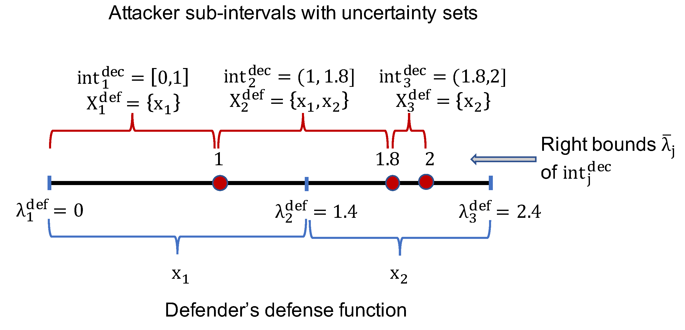An example of decomposing the deceptive range of ${\lambda }^{\mathrm{dec}}$ is shown in Figure 2.

5.1.2. Characteristics of Attacker Optimal Deception

We denote by M the number of attacker intervals. Given the division of the attacker’s deception range $\left\{in{t}_j^{\mathrm{dec}}\right\}$, we can divide the problem of attacker deception into M sub-problems. Each corresponds to a particular $in{t}_j^{\mathrm{dec}}$ where $j\in \{1,\cdots ,M\}$, as follows:

$$\begin{array}{c}\hfill \left({\overline{\mathbf{P}}}_{\mathbf{j}}^{\mathrm{dec}}\right):U_j^{a,*}=\underset{{\lambda }^{\mathrm{dec}}\in in{t}_j^{\mathrm{dec}}}{max}\underset{x_n\in {\mathbf{X}}_j^{\mathrm{def}}}{min}{U}^a(x_n,{\lambda }^{\mathrm{dec}})\end{array}$$

Lemma 8.

For each sub-problem (${\overline{\mathbf{P}}}_{\mathbf{j}}^{\mathrm{dec}}$) with respect to the deception sub-interval $in{t}_j^{\mathrm{dec}}$, the attacker optimal deception is to imitate the right-bound of $in{t}_j^{\mathrm{dec}}$, denoted by ${\overline{\lambda }}_j^{\mathrm{dec}}$.

The proof of Lemma 8 is derived based on the fact that the attacker’s utility $U^a({\mathbf{x}}_n,{\lambda }^{\mathrm{dec}})$ is increasing in ${\lambda }^{\mathrm{dec}}$. As a result, the attacker only has to search over the right bounds, $\left\{{\overline{\lambda }}_j^{\mathrm{dec}}\right\}$, of all intervals $\left\{in{t}_j^{\mathrm{dec}}\right\}$ to find the best one among the sub-problems that maximizes the attacker’s worst-case utility. We consider these bounds ${\overline{\lambda }}_j^{\mathrm{dec}}$ to be the deception candidates of the attacker. Let us assume $j^{opt}$ is the best deception choice for the attacker among these candidates, that is, the attacker will mimic the ${\overline{\lambda }}_{j^{opt}}^{\mathrm{dec}}$. We obtain the following observations about important properties of the attacker’s optimal deception, which we leverage to determine an optimal defense function later.

Our following Lemma 9 says that any non-optimal deception candidate for the attacker, ${\overline{\lambda }}_j^{\mathrm{dec}}\ne {\overline{\lambda }}_{j^{opt}}^{\mathrm{dec}}$, such that the max index of the defender strategy in the corresponding uncertainty set ${\mathbf{X}}_j^{\mathrm{def}}$, denoted by $n_j^{max}$, satisfies $n_j^{max}\le n_{j^{opt}}^{max}$, then the deception candidate ${\overline{\lambda }}_j^{\mathrm{dec}}$ is strictly less than ${\overline{\lambda }}_{j^{opt}}^{\mathrm{dec}}$, or equivalently, $j<j^{opt}$. Otherwise, $j^{opt}$ cannot be a best deception response.

Lemma 9.

For any $j\ne j^{opt}$ s.t. $n_j^{max}\le n_{j^{opt}}^{max}$, then ${\overline{\lambda }}_j^{\mathit{dec}}<{\overline{\lambda }}_{j^{opt}}^{\mathit{dec}}$, or equivalently, $j<j^{opt}$.

Proof. 

Lemma 9 can be proved by contradiction as follows. Let us assume if there is $j>j^{opt}$ such that $n_j^{max}\le n_{j^{opt}}^{max}$. According to Algorithm 2, for any attacker interval indices $j>j^{\prime }$, we have the min and max indices of the defender’s strategies in corresponding uncertainty sets must satisfy: $n_j^{min}\ge n_{j^{\prime }}^{min}$ and $n_j^{max}\ge n_{j^{\prime }}^{max}$, and they can not be both equal. That is because the intervals $\left\{in{t}_j^{\mathrm{dec}}\right\}$ returned by Algorithm 2 are sorted in a strictly increasing order. Therefore, if there is $j>j^{opt}$ such that $n_j^{max}\le n_{j^{opt}}^{max}$, it means $n_j^{min}>n_{j^{opt}}^{min}$ and $n_j^{max}=n_{j^{opt}}^{max}$. In other words, the uncertainty set ${\mathbf{X}}_j^{\mathrm{def}}\subset {\mathbf{X}}_{j^{opt}}^{def}$. Thus, we have the attacker’s optimal worst-case utility w.r.t deception intervals j and $j^{opt}$ must satisfy:

$$\begin{array}{cc}\hfill & U_{j^{opt}}^{a,*}=\underset{\mathbf{x}\in {\mathbf{X}}_{j^{opt}}^{\mathrm{def}}}{min}{U}^a(\mathbf{x},{\overline{\lambda }}_{j^{opt}}^{\mathrm{dec}})\le \underset{\mathbf{x}\in {\mathbf{X}}_j^{\mathrm{def}}}{min}{U}^a(\mathbf{x},{\overline{\lambda }}_{j^{opt}}^{\mathrm{dec}})<\underset{\mathbf{x}\in {\mathbf{X}}_j^{\mathrm{def}}}{min}{U}^a(\mathbf{x},{\overline{\lambda }}_j^{\mathrm{dec}})=U_j^{a,*}\hfill \end{array}$$

since $U^a(\mathbf{x},\lambda )$ is a strictly increasing function of $\lambda$3. This strict inequality shows that $j^{opt}$ cannot be an optimal deception for the attacker, concluding our proof for Observation 9.

Note that we denote right bounds of attacker intervals by $\{{\overline{\lambda }}_1^{\mathrm{dec}},\dots ,{\overline{\lambda }}_M^{\mathrm{dec}}={\lambda }^{max}\}$. Our Lemma 10 then says that if the max index of the defender strategy $n_{j^{opt}}^{max}$ in the set ${\mathbf{X}}_{j^{opt}}$ is equal to the max index of the whole defense set, N, then ${\overline{\lambda }}_{j^{opt}}^{\mathrm{dec}}$ is equal to the highest value of the entire deception range, i.e., ${\overline{\lambda }}_{j^{opt}}^{\mathrm{dec}}={\overline{\lambda }}_M={\lambda }^{max}$, or equivalently, $j^{opt}=M$.

Lemma 10.

If $n_{j^{opt}}^{max}=N$, then $j^{opt}=M$.

Proof. 

We also prove this observation using contradiction. Let us assume that $j^{opt}<M$. Again, according to Algorithm 2, for any $j>j^{\prime }$, we have $n_j^{min}\ge n_{j^{\prime }}^{min}$ and $n_j^{max}\ge n_{j^{\prime }}^{max}$, and they can not be both equal. Therefore, if $n_{j^{opt}}^{max}=N$, then for all $j>j^{opt}$, we have: $n_j^{max}=N$ and $n_j^{min}>n_{j^{opt}}^{min}$, which means ${\mathbf{X}}_j^{\mathrm{def}}\subset {\mathbf{X}}_{j^{opt}}^{\mathrm{def}}$. Therefore, if $j^{opt}<M$, then we obtain:

$$\begin{array}{cc}\hfill & U_{j^{opt}}^{a,*}=\underset{\mathbf{x}\in {\mathbf{X}}_{j^{opt}}^{\mathrm{def}}}{min}{U}^a(\mathbf{x},{\overline{\lambda }}_{j^{opt}}^{\mathrm{dec}})\le \underset{\mathbf{x}\in {\mathbf{X}}_M^{\mathrm{def}}}{min}{U}^a(\mathbf{x},{\overline{\lambda }}_{j^{opt}}^{\mathrm{dec}})<\underset{\mathbf{x}\in {\mathbf{X}}_M^{\mathrm{def}}}{min}{U}^a(\mathbf{x},{\overline{\lambda }}_M^{\mathrm{dec}})=U_M^{a,*}\hfill \end{array}$$

which shows that $j^{opt}$ cannot be an optimal deception of the attacker, concluding the proof of Lemma 10. □

Remark 1.

According to Lemmas 9 and 10, we can easily determine which deception choices among the set$\{{\overline{\lambda }}_1^{\mathrm{dec}},\dots ,{\overline{\lambda }}_M^{\mathrm{dec}}\}$cannot be an optimal attacker deception, regardless of defense strategies$\{{\mathbf{x}}_1,\dots ,{\mathbf{x}}_N\}$. These non-optimal choices are determined as follows: the deception choice${\overline{\lambda }}_j$can not be optimal for:

• Anyjsuch that there is a$j^{\prime }>j$with$n_{j^{\prime }}^{max}\le n_j^{max}$
• Any$j<M$such that$n_j^{max}=N$

For any other choices${\overline{\lambda }}_j^{\mathrm{dec}}$, there always exists defense strategies$\{{\mathbf{x}}_1,\cdots ,{\mathbf{x}}_N\}$such that${\overline{\lambda }}_j^{\mathrm{dec}}$is an optimal attacker deception.

5.2. Finding Optimal Defense Function ${\mathcal{H}}^I$ Given Fixed I: Divide-and-Conquer

Given a set of sub-intervals $\mathbf{I}$, we aim at finding optimal defense function ${\mathcal{H}}^I$ or equivalently, strategies ${\mathbf{X}}^{\mathrm{def}}=\{{\mathbf{x}}_1,{\mathbf{x}}_2,\cdots ,{\mathbf{x}}_N\}$ corresponding to these sub-intervals. According to previous analysis on the attacker’s deception adaptation, since the attacker’s best deception is one of the bounds $\{{\overline{\lambda }}_1^{\mathrm{dec}},\cdots ,{\overline{\lambda }}_M^{\mathrm{dec}}\}$, we propose to decompose the problem of finding an optimal defense function ${\mathcal{H}}^I$ into multiple sub-problems ${\mathbf{P}}_{\mathbf{j}}^{\mathrm{counter}}$, each corresponds to a particular best deception choice for the attacker. In particular, for each sub-problem ${\mathbf{P}}_{\mathbf{j}}^{\mathrm{counter}}$, we attempt to find ${\mathcal{H}}^{\mathbf{I}}$ such that ${\overline{\lambda }}_j^{\mathrm{dec}}$ is the best response of the attacker. As discussed in the remark of previous section, we can easily determine which sub-problem ${\mathbf{P}}_{\mathbf{j}}^{\mathrm{counter}}$ is not feasible. For any feasible optimal deception candidate $j^{\mathrm{fea}}$, i.e., ${\mathbf{P}}_{{\mathbf{j}}^{\mathrm{fea}}}^{\mathrm{counter}}$ is feasible, ${\mathbf{P}}_{{\mathbf{j}}^{\mathrm{fea}}}^{\mathrm{counter}}$ can be formulated as follows:

$$\begin{array}{cc}\hfill \left({\mathbf{P}}_{{\mathbf{j}}^{\mathrm{fea}}}^{\mathrm{counter}}\right):\underset{{\mathcal{H}}^{\mathbf{I}}}{max}& U^d({\mathcal{H}}^{\mathbf{I}},{\overline{\lambda }}_{j^{\mathrm{fea}}}^{\mathrm{dec}})\hfill \\ \hfill \mathrm{s}.\mathrm{t}.& \underset{\mathbf{x}\in {\mathbf{X}}_{j^{\mathrm{fea}}}^{\mathrm{def}}}{min}{U}^a(\mathbf{x},{\overline{\lambda }}_{j^{\mathrm{fea}}}^{\mathrm{dec}})\ge \underset{\mathbf{x}\in {\mathbf{X}}_j^{\mathrm{def}}}{min}{U}^a(\mathbf{x},{\overline{\lambda }}_j^{\mathrm{dec}}),\forall j\hfill \end{array}$$

where $U^d({\mathcal{H}}^{\mathbf{I}},{\overline{\lambda }}_{j^{\mathrm{fea}}}^{\mathrm{dec}})$ is the defender’s utility when the defender commits to ${\mathcal{H}}^{\mathbf{I}}$ and the attacker plays ${\overline{\lambda }}_{j^{\mathrm{fea}}}^{\mathrm{dec}}$. The constraints in $\left({\mathbf{P}}_{{\mathbf{j}}^{\mathrm{fea}}}^{\mathrm{counter}}\right)$ guarantee that the attacker’s worst-case utility for playing ${\overline{\lambda }}_{j^{\mathrm{fea}}}^{\mathrm{dec}}$ is better than playing other ${\overline{\lambda }}_j^{\mathrm{dec}}$. Finally, our Propositions 2 and 3 determine an optimal solution for (${\mathbf{P}}_{{\mathbf{j}}^{\mathrm{fea}}}^{\mathrm{counter}}$).

Proposition 2

(Sub-problem ${\mathbf{P}}_{{\mathbf{j}}^{\mathrm{fea}}}^{\mathrm{counter}}$). If $n_{j^{\mathrm{fea}}}^{max}<N$, the best defense function for the defender is determined as follows:

• For all $n>n_{j^{\mathrm{fea}}}^{max}$, choose ${\mathbf{x}}_n={\mathbf{x}}_{>}^{*}$ where ${\mathbf{x}}_{>}^{*}$ is an optimal solution of the following optimization problem:

  $$\begin{array}{cc}\hfill & {min}_{\mathbf{x}\in \mathbf{X}}{U}^a(\mathbf{x},{\lambda }^{max})\hfill \end{array}$$
• For all $n\le n_{j^{\mathrm{fea}}}^{max}$, choose ${\mathbf{x}}_n={\mathbf{x}}_{<}^{*}$ where ${\mathbf{x}}_{<}^{*}$ is the optimal solution of the following optimization problem:

  $$\begin{array}{cc}\hfill U_{*}^d={max}_{\mathbf{x}\in \mathbf{X}}& U^d(\mathbf{x},{\overline{\lambda }}_{j^{\mathrm{fea}}}^{\mathrm{dec}})\hfill \\ \hfill \mathrm{s}.\mathrm{t}.& U^a(\mathbf{x},{\overline{\lambda }}_{j^{\mathrm{fea}}}^{\mathrm{dec}})\ge U^a({\mathbf{x}}_{>}^{*},{\lambda }^{max})\hfill \end{array}$$

By following the above defense function, an optimal deception of the attacker is to mimic ${\overline{\lambda }}_{j^{\mathrm{fea}}}^{\mathrm{dec}}$, and the defender obtains an utility of $U_{*}^d$.

Proof. 

First, we show that the attacker optimal deception response is to ${\overline{\lambda }}_{j^{\mathrm{fea}}}^{\mathrm{dec}}$. Indeed, we have the uncertainty set ${\mathbf{X}}_{j^{\mathrm{fea}}}^{\mathrm{def}}\equiv \left\{{\mathbf{x}}_{<}^{*}\right\}$ because the defender plays ${\mathbf{x}}_n={\mathbf{x}}_{<}^{*}$ for all $n\le n_{j^{\mathrm{fea}}}^{max}$. In addition, for all j such that $n_j^{max}>n_{j^{\mathrm{fea}}}^{max}$, the uncertainty set ${\mathbf{X}}_j^{\mathrm{def}}$ contains ${\mathbf{x}}_{>}^{*}$. Therefore, we have the attacker worst-case utility satisfying:

$$\begin{array}{c}\hfill U_j^{a,*}\le U^a({\mathbf{x}}_{>}^{*},{\overline{\lambda }}_j^{\mathrm{dec}})\le U^a({\mathbf{x}}_{>}^{*},{\lambda }^{max})\le U^a({\mathbf{x}}_{<}^{*},{\overline{\lambda }}_{j^{\mathrm{fea}}}^{\mathrm{dec}})=U_{j^{\mathrm{fea}}}^{a,*}\end{array}$$

Furthermore, for all j such that $n_j^{max}\le n_{j^{\mathrm{fea}}}^{max}$, we have $j\le j^{\mathrm{fea}}$ according to Observation 9. Thus, we obtain:

$$\begin{array}{cc}\hfill & U_j^{a,*}=U^a({\mathbf{x}}_{<}^{*},{\overline{\lambda }}_j^{\mathrm{dec}})\le U^a({\mathbf{x}}_{<}^{*},{\overline{\lambda }}_{j^{\mathrm{fea}}})=U_{j^{\mathrm{fea}}}^{a,*}\hfill \end{array}$$

Based on the above defense function and the fact that the attacker will choose ${\overline{\lambda }}_{j^{\mathrm{fea}}}^{\mathrm{dec}}$, the defender receives an utility of $U_{*}^d$. Next, we prove that this is the best the defender can obtain by showing that any defense function $\{x_1^{\prime },\dots ,x_N^{\prime }\}$ such that $j^{\mathrm{fea}}$ is the attacker’s best response will lead to a defender utility less than $U_{*}^d$. Indeed, since $n_{j^{\mathrm{fea}}}^{max}<N$, it means $j^{\mathrm{fea}}<M$ or in other words, ${\overline{\lambda }}_{j^{\mathrm{fea}}}^{\mathrm{dec}}<{\overline{\lambda }}_M={\lambda }^{max}$. On the other hand, since ${\overline{\lambda }}_{j^{\mathrm{fea}}}^{\mathrm{dec}}$ is the best choice of the attacker, the following inequality must hold:

$$\begin{array}{cc}\hfill & U_{j^{\mathrm{fea}}}^{a,*}\ge U_M^{a,*}=\underset{\mathbf{x}\in {\mathbf{X}}_M^{\mathrm{def}}}{min}{U}^a(\mathbf{x},{\lambda }^{max})\ge \underset{\mathbf{x}\in \mathbf{X}}{min}{U}^a(\mathbf{x},{\lambda }^{max})\hfill \end{array}$$

This means that any defense function $\{x_1^{\prime },\dots ,x_k^{\prime }\}$ such that $j^{\mathrm{fea}}$ is the attacker’s best response has to satisfy the above inequality. As defined, $U_{*}^d$ is the highest utility for the defender among these defense functions that satisfy the above inequality. □

Proposition 3

(Sub-problem ${\mathbf{P}}_{{\mathbf{j}}^{\mathrm{fea}}}^{\mathrm{counter}}$). If $n_{j^{\mathit{fea}}}^{max}=N$, the best counter-deception of the defender can be determined as follows: for all n, we set: ${\mathbf{x}}_n=\widehat{\mathbf{x}}$ where $\widehat{\mathbf{x}}$ is an optimal solution of

$${max}_{\mathbf{x}\in \mathbf{X}}{U}^d(\mathbf{x},{\lambda }^{max})$$

By following this defense function, the attacker’s best deception is to mimic ${\lambda }^{max}$ and the defender obtains an utility of $U^d(\widehat{\mathbf{x}},{\lambda }^{max})$.

Proof. 

First, we observe that given $\widehat{\mathbf{x}}$, ${\overline{\lambda }}_{j^{\mathrm{fea}}}$ is the best response of the attacker. Indeed, since $j^{\mathrm{fea}}=M$ or equivalently ${\overline{\lambda }}_{j^{\mathrm{fea}}}={\lambda }^{max}$ according to Observation 10, we have:

$$\begin{array}{c}\hfill U_{j^{\mathrm{fea}}}^{a,*}=U^a(\widehat{\mathbf{x}},{\lambda }^{max})\ge U^a(\widehat{\mathbf{x}},{\overline{\lambda }}_j^{\mathrm{dec}})=U_j^{a,*},\forall j\end{array}$$

Second, since ${\overline{\lambda }}_{j^{\mathrm{fea}}}={\lambda }^{max}$, then for any defense function such that ${\overline{\lambda }}_{j^{\mathrm{fea}}}$ is the best deception choice of the attacker, the resulting utility for the defender must be no more than:

$$\begin{array}{cc}\hfill & {max}_{\mathbf{x}\in {\mathbf{X}}_{j^{\mathrm{fea}}}^{\mathrm{def}}}{U}^d(\mathbf{x},{\lambda }^{max})\le {max}_{\mathbf{x}\in \mathbf{X}}{U}^d(\mathbf{x},{\lambda }^{max})\hfill \end{array}$$

regardless of the learning outcome ${\lambda }^{\mathrm{learnt}}\in [{\lambda }^{max}-\delta ,{\lambda }^{max}+\delta ]$. This is because the defender eventually plays one of the defense strategies in the set ${\mathbf{X}}_{j^{\mathrm{fea}}}^{\mathrm{def}}$. The RHS is the defender’s utility obtained by playing the counter-deception specified by the proposition. □

Based on Propositions 2 and 3, we can easily find the optimal counter-deception by choosing the solution of the sub-problem that provides the highest defender utility.

5.3. Completing the Proof of Theorem 3

According to Propositions 2 and 3, given an interval set $\mathbf{I}$, the resulting defense function will only lead the defender to play either $\{{\mathbf{x}}_{>}^{*},{\mathbf{x}}_{<}^{*}\}$ or $\left\{\widehat{\mathbf{x}}\right\}$, whichever provides a higher utility for the defender. Based on this result, our Theorem 3 then identifies an optimal interval set, and corresponding optimal defense strategies, as we prove below.

First, we will show that if the defender follows the defense function specified in Theorem 3, then the attacker’s optimal deception is to mimic ${\lambda }^{*}$. Indeed, if ${\lambda }^{*}={\lambda }^{max}$, then since the defender always plays ${\mathbf{x}}^{*}$, the attacker’s optimal deception is to play ${\lambda }^{*}={\lambda }^{max}$ to obtain a highest utility $U^a({\mathbf{x}}^{*},{\lambda }^{max})$.

On the other hand, if ${\lambda }^{*}<{\lambda }^{max}$, we consider two cases:

Case 1, if ${\lambda }^{max}-2\delta \le {\lambda }^{*}<{\lambda }^{max}$, then the intervals of the attackers are $in{t}_1^{\mathrm{dec}}=[0,{\lambda }^{*}]$ and $in{t}_2^{\mathrm{dec}}=({\lambda }^{*},{\lambda }^{max}]$. The corresponding uncertainty sets are ${\mathbf{X}}_1^{\mathrm{def}}=\left\{{\mathbf{x}}_1\right\}$ and ${\mathbf{X}}_2^{\mathrm{def}}=\{{\mathbf{x}}_1,{\mathbf{x}}_2\}$. In this case, the attacker’s optimal deception is to mimic ${\lambda }^{*}$, since:

$$\begin{array}{cc}\hfill & \underset{\mathbf{x}\in {\mathbf{X}}_1^{\mathrm{def}}}{min}{U}^a(\mathbf{x},{\lambda }^{*})=U^a({\mathbf{x}}^{*},{\lambda }^{*})\ge U^a({\mathbf{x}}_2,{\lambda }^{max})\ge \underset{\mathbf{x}\in {\mathbf{X}}_2^{\mathrm{def}}}{min}{U}^a(\mathbf{x},{\lambda }^{max})\hfill \end{array}$$

Case 2, if ${\lambda }^{*}<{\lambda }^{max}-2\delta$, then the corresponding intervals for the attacker are $in{t}_1^{\mathrm{dec}}=[0,{\lambda }^{*}]$, $in{t}_2^{\mathrm{dec}}=({\lambda }^{*},{\lambda }^{*}+2\delta ]$, and $in{t}_3^{\mathrm{dec}}=({\lambda }^{*}+2\delta ,{\lambda }^{max}]$. These intervals of the attacker have uncertainty sets ${\mathbf{X}}_1^{\mathrm{def}}=\left\{{\mathbf{x}}_1\right\}$, ${\mathbf{X}}_2^{\mathrm{def}}=\{{\mathbf{x}}_1,{\mathbf{x}}_2\}$, and ${\mathbf{X}}_3^{\mathrm{def}}=\left\{{\mathbf{x}}_2\right\}$, respectively. The attacker’s best deception is thus to mimic ${\lambda }^{*}$, since the attacker’s worst-case utility is ${min}_{\mathbf{x}\in {\mathbf{X}}_1^{\mathrm{def}}}{U}^a(\mathbf{x},{\lambda }^{*})=U^a({\mathbf{x}}^{*},{\lambda }^{*})$, and

$$\begin{array}{cc}\hfill & U^a({\mathbf{x}}^{*},{\lambda }^{*})\ge U^a({\mathbf{x}}_2,{\lambda }^{max})\ge {min}_{\mathbf{x}\in {\mathbf{X}}_2}{U}^a(\mathbf{x},{\lambda }^{*}+2\delta )\hfill \\ \hfill & U^a({\mathbf{x}}^{*},{\lambda }^{*})\ge U^a({\mathbf{x}}_2,{\lambda }^{max})={min}_{\mathbf{x}\in {\mathbf{X}}_3}{U}^a(\mathbf{x},{\lambda }^{max})\hfill \end{array}$$

Now, since the attacker’s best deception is to mimic ${\lambda }^{*}$, according to the above analysis, the uncertainty set is ${\mathbf{X}}_1^{\mathrm{def}}=\{{\mathbf{x}}_1={\mathbf{x}}^{*}\}$, thus the defender will play ${\mathbf{x}}^{*}$ in the end, leading to an utility of $U^d({\mathbf{x}}^{*},{\lambda }^{*})$. This is the highest possible utility that the defender can obtain since both optimization problems presented in Propositions 2 and 3 are special cases of (${\mathbf{P}}^{\mathrm{counter}}$) when we fix the variable $\lambda ={\lambda }^{max}$ (for Proposition 3) or $\lambda ={\overline{\lambda }}_{j^{\mathrm{fea}}}$ (for Proposition 2).

6. Experimental Evaluation

Our experiments are run on a 2.8 GHz Intel Xeon processor with 256 GB RAM. We use $\mathtt{Matlab}$ (https://www.mathworks.com, accessed on 1 October 2022) to solve non-linear programs and $\mathtt{Cplex}$ (https://www.ibm.com/analytics/cplex-optimizer, accessed on 1 October 2022) to solve $\mathtt{MILP}$s involved in the evaluated algorithms. We use a value of ${\lambda }^{max}=5$ in all our experiments (except in Figure 3g,h), and discretize the range $[0,{\lambda }^{max}]$ using a step size of $0.2$: $\lambda \in \{0,0.2,\dots ,{\lambda }^{max}\}$. We use the covariance game generator, $\mathtt{GAMUT}$ (http://gamut.stanford/edu, accessed on 1 October 2022) to generate rewards and penalties of players within the range of $[1,10]$ (for attacker) and $[-10,-1]$ (for defender). GAMUT takes as input a covariance value $r\in [-1,0]$ which controls the correlations between the defender and the attacker’s payoff. Our results are averaged over 50 runs. All our results are statistically significant under bootstrap-t ($p=0.05$).

Algorithms. We compare three cases: (i) $\mathtt{Non}-\mathtt{Dec}$: the attacker is non deceptive and the defender also assumes so. As a result, both play Strong Stackelberg equilibrium strategies; (ii) $\mathtt{Dec}-\delta$: the attacker is deceptive, while the defender does not handle the attacker’s deception (Section 4). We examine different uncertainty ranges by varying values of $\delta$; and (iii) $\mathtt{Dec}-\mathtt{Counter}$: the attacker is deceptive while the defender tackle the attacker’s deception (Section 5).

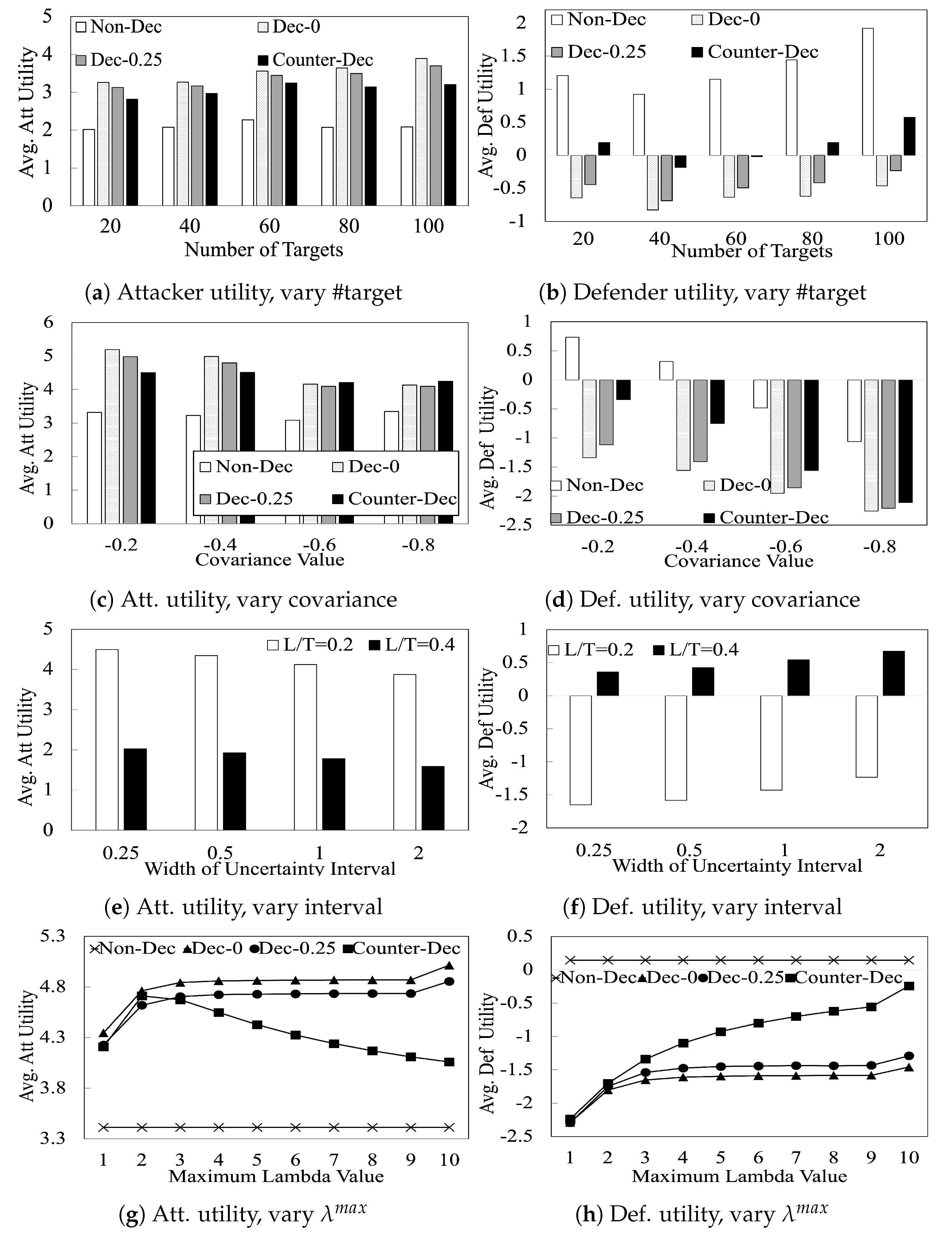
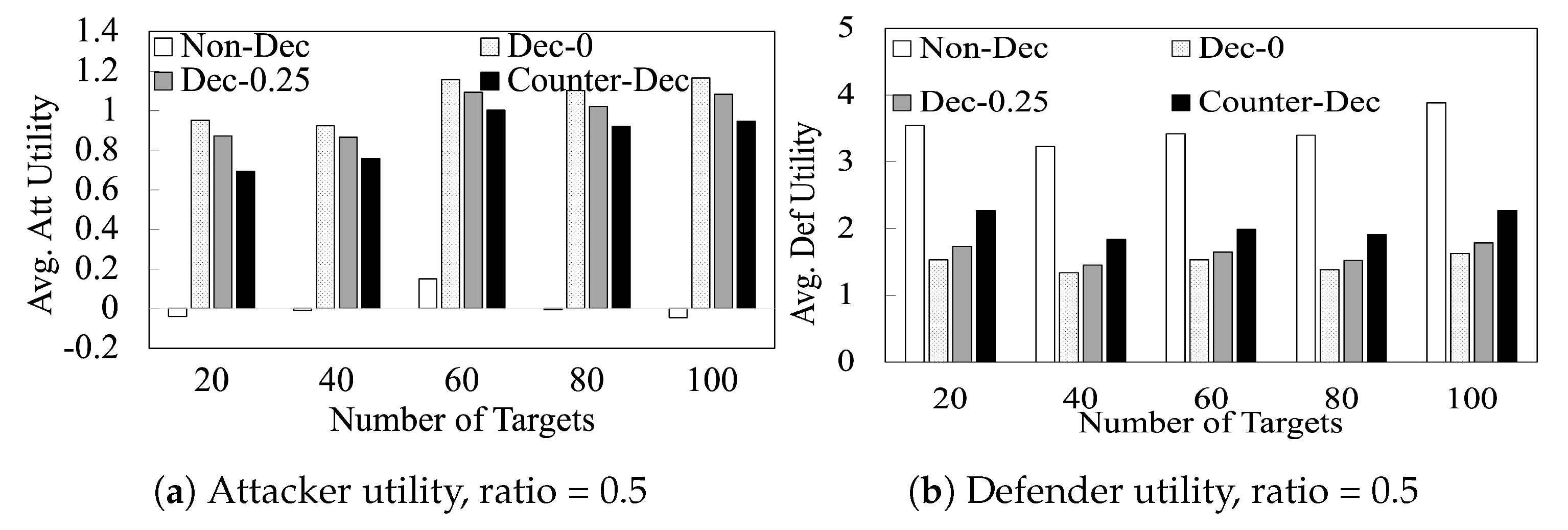
Figure 3a,b compare the performance of our algorithms with increasing number of targets. These figures show that (i) the attacker benefits by playing deceptively ($\mathtt{Dec}-\mathtt{0}$ achieves 61% higher attacker utility than $\mathtt{Non}-\mathtt{Dec}$); (ii) the benefit of deception to the attacker is reduced when the attacker is uncertain about the defender’s learning outcome. In particular, $\mathtt{Dec}-\mathtt{0.25}$ achieves 4% lesser attacker utility than $\mathtt{Dec}-\mathtt{0}$; (iii) the defender suffers a substantial utility loss due to the attacker’s deception and this utility loss is reduced in the presence of the attacker’s uncertainty; and finally, (iv) the defender benefits significantly (in their utility) by employing counter-deception against a deceptive attacker.

In Figure 3c,d, we show the performance of our algorithms with varying r (i.e., covariance) values. In zero-sum games (i.e., $r=-1$), the attacker has no incentive to be deceptive [4]. Therefore, we only plot the results of $r\in [-0.2,-0.8]$ with a step size of $0.2$. This figure shows that when r gets closer to $-1.0$ (which implies zero-sum behavior), the attacker’s utility with deception (i.e., $\mathtt{Dec}-\mathtt{0}$ and $\mathtt{Dec}-\mathtt{0.25}$) gradually moves closer to its utility with $\mathtt{Non}-\mathtt{Dec}$, reflecting that the attacker has less incentive to play deceptively. Furthermore, the defender’s average utility in all cases gradually decreases when the covariance value gets closer to $-1.0$. This results show that in $\mathtt{SSG}$s, the defender’s utility is always governed by the adversarial level (i.e., the payoff correlations) between the players, regardless of whether the attacker is deceptive or not.

Figure 3e,f compare the attacker and defender utilities with varying uncertainty range, i.e., $\delta$ values, on 60-target games. These figures show that attacker utilities decrease linearly with increasing values of $\delta$. On the other hand, defender utilities increase linearly with increasing values of $\delta$. This is reasonable as increasing $\delta$ corresponds to a greater width of the uncertainty interval that the attacker has to contend with. This increased uncertainty forces the attacker to play more conservatively, thereby leading to decreased utilities for the attacker and increased utilities for the defender.

In Figure 3g,h, we analyze the impact of varying ${\lambda }^{max}$ on the players’ utilities in 60-target games. These figures show that (i) with increasing values of ${\lambda }^{max}$, the action space of a deceptive attacker increases, hence, the attacker utility increases as a result ($\mathtt{Dec}-\mathtt{0}$, $\mathtt{Dec}-\mathtt{0.25}$ in both sub-figures); (ii) When this ${\lambda }^{max}$ is close to zero, the attacker is limited to a less-strategic-attack zone and thus the defender’s strategies have less influence on how the attacker would response. The defender thus receives a lower utility when ${\lambda }^{max}$ gets close to zero; and (iii) most importantly, the attacker utility against a counter-deceptive defender decreases with increasing values of ${\lambda }^{max}$. This result shows that when the defender plays counter-deception, the attacker can actually gain more benefit by committing to a more limited deception range.

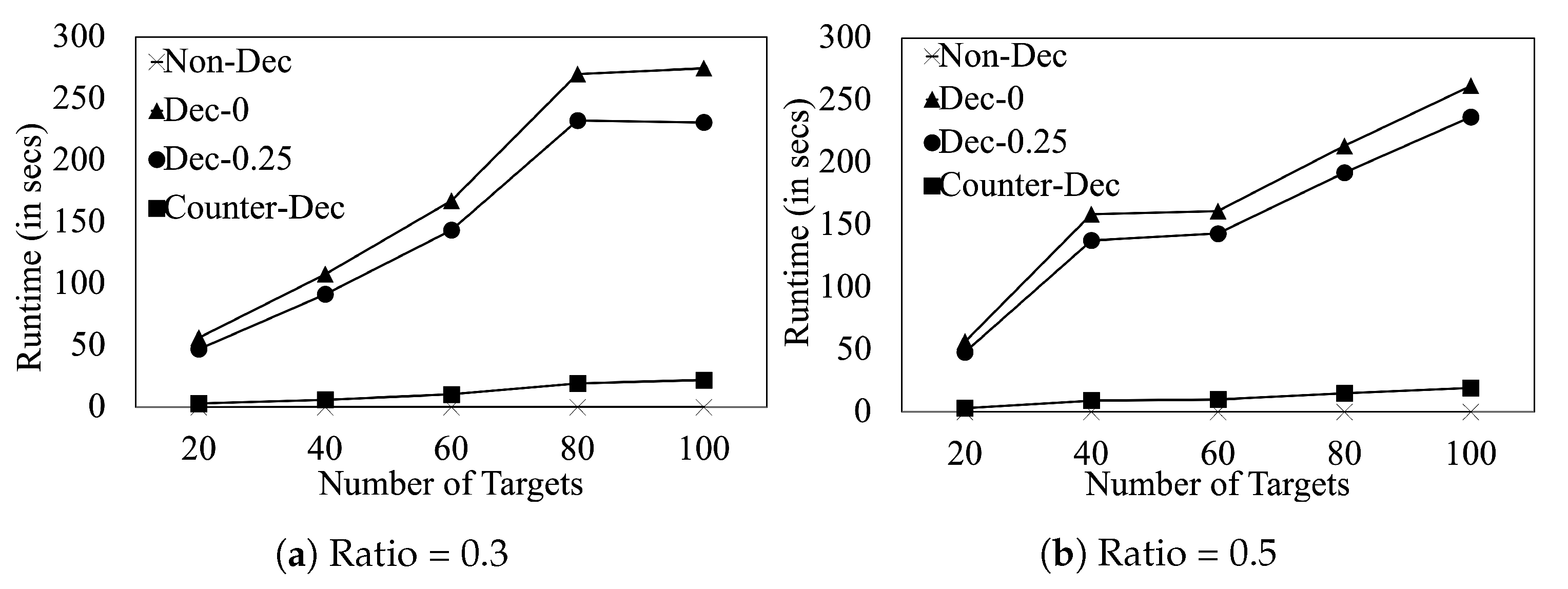
Finally, we evaluate the runtime performance of our algorithms in Figure 4. We provide results for resource-to-target ratio $\frac{L}{T}=0.3$ and $0.5$. This figure shows that (i) even on 100 target games, $\mathtt{Dec}-\mathtt{0}$ finishes in ∼5 min. (ii) Due to the simplicity of the proposed counter-deception algorithm, $\mathtt{Counter}-\mathtt{Dec}$ finishes in 13 s on 100 target games.

Additional Experiment Results

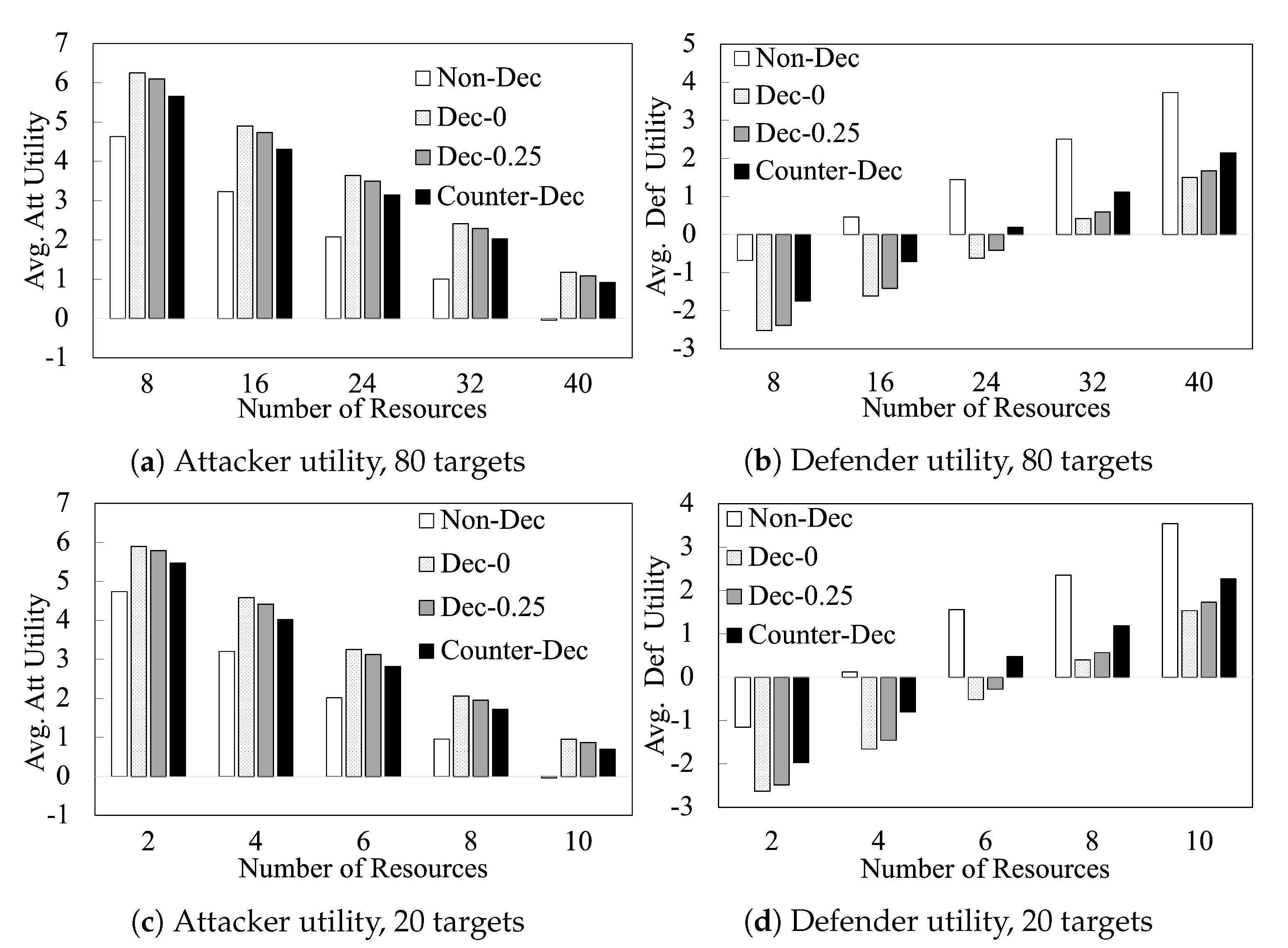
Figure 5 shows the performance of our algorithms as we vary the number of resources L on 80-target games and 20-target games. This figure shows that the benefits of deception and counter-deception to the players are observed consistently when varying L. It shows that (i) the defender (attacker) utilities steadily increase (decrease) with increasing L; and (ii) the trends observed between the different algorithms in Figure 5 are observed consistently at different values of L. In Figure 6, we compare different algorithms with increasing number of targets when $\frac{L}{T}=0.5$. We observe similar trends in these additional results.

7. Conclusions

This paper provides a comprehensive analysis of the attacker deception and defender counter-deception under uncertainty. Our algorithms are developed based on the decomposibility of the attacker’s deception space and the discretization of the defender’s learning outcome. Our key finding is that the optimal counter-deception defense solution only depends on the common knowledge of players about the uncertainty range of the defender’s learning outcome. Finally, our extensive experiments show the effectiveness of our counter-deception solutions in handling the attacker’s deception.

As for future work, this article focus on the attacker deception and defender counter-deception in the context of the Quantal Response model, which only has a single model parameter. Given promising results of this article, investigating the attacker deception in more complex model settings such as neural nets would be interesting future direction.