1. Introduction
In the year 2015, a theory of games was proposed that does not use real-valued payoffs, but rather achieves optimization using stochastic orders on rewards that are probability distributions. Ever since, a couple of intricacies—even pathologies—have been found in such generalized games, and this article is a compilation of the recent findings, advantages, but also pitfalls to avoid when working with game theory over the abstract space of probability distributions. The theory was originally motivated by applications of games in security risk management, where payoffs are hardly crisp or accurately quantifiable; thus, there is a desire to include uncertainty in the game model already before computing solutions. This uncertainty is not in the actions, as is the case for refined equilibrium concepts such as trembling hands or perfect equilibria, but rather in the rewards themselves. Reducing the random outcomes to their averages (expectations) or other representative statistics necessarily sacrifices information that is, in security risk management, generally scarce already. This creates an additional desire to use information about possible effects of an action to the maximum extent available.
The story behind all our upcoming considerations evolves around a defending player 1 who seeks to guard a system against a rational or irrational attacker from outside. In a typical generic setting, the defender may be the chief security officer (CISO) of some large enterprise, and is committed to business continuity management and the most important line of defense against external competitors and adversaries (hackers, and others).
In this situation, the defender often has to consider multiple goals simultaneously, including damage or loss of sensitive data, the possibility of physical damage to equipment and people (for example, if a production line gets hacked and a robot damages goods or hurts a person), up to issues of reputation, damage compensations, and many others. A security game in such contexts is thus generally a multi-criteria optimization problem, with hardly quantifiable losses to be minimized. For example, if a production line stops for some time, we may have an average estimate of how much that costs per hour, but this value is not quantifiable in an exact way, since the duration of the outage remains random. Insurance and actuarial science [
1,
2] offer lots of probabilistic models to describe extreme events (the whole theory of extreme value distributions, up to catastrophe theory, can be useful here), but game theory can become difficult to apply if we need to define real-valued, and hence exact, utility functions for optimization.
Summarizing the challenges, we have the following situation: A player is minimizing losses by taking strategic action. The losses are inherently random, and admit a quantification only up to the point of modeling a probability distribution that is conditional on the other players’ actions. Specifically, we are unable to give an exact valuation of payoffs to a player due to intrinsic uncertainty. We assume, however, that we can reasonably model the players’ random payoff as a (conditional) probability distribution, with loss distribution models that are assumed to exist and be known for the given application context. As an example (taken from [
3]), such a conditional distribution can be the probability to “catch an intruder”, conditional on the (random) location of the security guard to be at the same location (by coincidence). Similar games have been proposed for border protection, airport protection and coast guarding [
4].
Besides the problem with uncertain revenues, some additional quantities that are difficult to bring into classical game models may be interesting. For example, since games typically optimize an average (expected) payoff, what are the chances of receiving more or less than this optimal average? This is important to know when buying insurance or building up backup resources, and is non-trivial to handle with classical game models. We discuss this situation as a concrete motivation for the generalized class of games in
Section 1.3.
1.1. Our Contribution
This study compiles recent work, findings and progress towards a theory of games for strategic decision making in non-cooperative situations, when consequences are intrinsically random and real valued (and hence crisp) payoff values are not available or are unreliable. This is essentially different from situations in which the imprecision is in the gameplay, such as trembling hands or perfect equilibria capture [
5,
6], and is also different from situations in which the uncertainty is about the adversary, such as Bayesian games [
7] cover by making assumptions about different types of players, e.g., based on levels of rationality [
8]. Defining games with “uncertain opponents” technically leads to uncertain utilities, as we consider, but the optimization itself is generally again over real values being expectations of (conditional) distributions. We intentionally want to avoid derandomization by averaging, since the expectation
contains less information than the random variable
U. In situations in which information is notoriously scarce, such as in security, unnecessary loss of information should be avoided. This is a common circumstance in risk management, where qualitative and overly precise valuations of an actions consequence are not only hard, but even explicitly discouraged [
9]. As an illustration, let us consider quantitative risk management in engineering. In this context, a risk manager makes a list of possible threats to its assets (enterprise business values, human beings or similar), where each threat, if it manifests in reality, may have an impact (e.g., monetary losses, reputational damages, etc.), and occurs with a likelihood to be estimated. The term “risk” is defined by a simple formula to be
and, provided that the risk manager can assign reliable values to both variables, nicely lends itself to optimization and game theory [
10] (indeed (
1) is interpretable as “expected damage” and can be taken as an adversary’s expected utility). If the threats are caused by a rational adversary trying to hack or otherwise hit a system, the threat list is nothing else than an action set of a hostile opponent. For the defender, engaging as the other player in the game has its own action set to protect against the possible threats. Risk management standards such as ISO27000 or ISO31000 provide long lists of actions (termed “controls” in this context), which are the defender’s actions to choose from strategically. The above formula can then be operationalized by playing a
non-cooperative game between two players, featuring the defender versus the attacker. The player’s expected utility can be taken directly as the risk = impact × likelihood. From the defender’s perspective, the “likelihood” would be the (optimized) probabilities of actions taken by the opponent, which is nothing other than a mixed equilibrium strategy. Likewise, the defender’s equilibrium then becomes an optimal randomized choice of actions to protect against all threats simultaneously. This mixed equilibrium is then convertible into an optimal resource allocation strategy for the defender, thus providing a provably optimal use of (typically scarce) defense budgets, against a rationally and strategically acting adversary. Recent work on game theoretic cyber security has independently pointed out the lack of consensual interpretations of mixed strategies in security, and our work addresses the resource allocation- and mixed strategy interpretation problem, both noted by [
11], on a common ground. Reference [
3] provided an interesting application for security surveillance monitoring, where the optimization must consider multiple criteria, even including the coverage level of the surveillance, but also the level of inconvenience that surveillance may cause to people at work.
Game theory offers powerful possibilities in letting us quantify likelihoods for risk management directly as optimal choice rules, for example, or interpreting mixed strategies as optimal resource allocation rules. However, the difficulty of applying games over real values is the need to “accurately quantify” the impact, which some authors even discourage in light of much and reliable data to be available. Reference [
9] explains this recommendation using an example of the decision about whether or not to buy protection against lightning strikes. Based on long-term statistical evidence, the likelihood of a lightning strike is accurately quantifiable (to be ≈
in the region around Munich/Germany), thus providing a seemingly reliable value for the risk Formula (
1). Similarly, the impact of a lightning strike is also not difficult to quantify, since we most likely know how expensive a repair to the facility would be. Thus, despite both values being accurately estimable (e.g., 10,000
$), their product numerically evaluates to an expected loss of ≈
. Basing a decision on this value to not invest in lightning protection is clearly implausible, and this example (among many others that are similar), leads to official recommendations to not estimate probabilities or impacts with seeming precision numerically, where there is no absolute accuracy.
The problem appears more widespread than only in the risk-management context, since any strategic decision under uncertain consequences of actions will need a well-founded account for uncertainty. For example, the effects of fake news spreading over social media certainly call for strategic intervention, but the effect of campaigns against fake news and disinformation are easily quantified in terms of costs, but are almost impossible to quantify in terms of effects. This makes the definition of crisp, i.e., real-valued utilities, generally hard in many practical instances of security management, and creates a need for a more general concept of games that can work with vague, fuzzy or generally uncertain outcomes of strategic actions.
This work, and its contributions, are thus motivated by the following five aspects collected from practical project work, which touch upon all of the above points:
First, the quantification of impacts for strategic optimization of actions should be avoided by official recommendations [
9]. Our work addresses this by letting games be played over uncertain utility values.
Second, strategic interventions in non-cooperative situations where the response dynamics is unknown, intrinsically uncertain or simply not describable in precise mathematical terms, such as social risk response—for example, [
12,
13]—may not lend themselves to the definition of crisp values. Agent-based simulations, as one possibility to anticipate social or community replies to actions of authorities, deliver a multitude of possible scenarios, and compiling a single value as a utility to optimize actions and interventions would be accompanied by a considerable loss of valuable information. Games using probability distributions are “conservative” here in using all information embodied in random simulations (e.g., Monte Carlo) for decision making. This also relates our work to empirical game theory, making statistical models such as those in actuarial science [
1,
14] useful for strategic decision making using games.
Third, optimizing averages offers no information, nor guarantee, about the fluctuations around the optimal mean. If the game is played to minimize the “expected damage”, one may consider buying insurance to cover for such expected losses. However, what if the game overshoots the losses in one or several rounds? How much more than the expected loss should we anticipate to buy insurance for? Real-valued game models are only concerned with optimizing the average, but do not give information about how “stable” this average outcome is. Playing the game over the whole distribution object, we can also consider the variance, skewness and other properties of the distribution in the decision-making process. One such property is the disappointment rate, which would lead to a discontinuous utility function in a real-valued instance of a game, and hence Nash equilibria may no longer exist. A contribution of this work is showing how probability distributions for payoffs in a game model can avoid such existence issues, and how to play games not only for the best outcome, but also for the least disappointment. This is a new form of equilibrium refinement, which much other work (not only in security) approaches by perfect equilibria or other (more technical) means.
Fourth, it has long been recognized that the utility maximization paradigm is not necessarily consistent with human decision making [
15]. Procedural theories, prospect theory and many other paradigms of decision making have been proposed ever since. As an example, reference [
3] has proposed a method to define utilities with regard to subjective risk appetite (aversion or affinity to risk). This construction leads to vector-valued utility functions, and recent work [
16] has demonstrated that such games do not necessarily have Nash equilibria. One contribution of this work is showing a proper solution concept in this case.
Finally, along the lines of vector-optimization, multi-criteria games are long known, and concepts such as Pareto–Nash equilibria are definable and useful [
17]. However, Pareto optimization needs a weighting among the multitude of criteria to scalarize the utility and thereby reduce the problem to a game with an aggregate, but scalar, utility. Since the lexicographic order is known to not be representable by a continuous real-valued function, this work contributes a method of defining an equilibrium over games with multiple goals in strict priority. A domain of practical application is in robotics, where the first priority is to avoid human coworkers being hurt by a malfunctioning robot, and the cost and functional correctness of the robot come as secondary and ternary goals.
The contributions made here, relative to related work, are as follows:
The proposal to model utilities not only as numbers, but whole distributions. This was first proposed in [
18], and applied in [
3,
10,
19]. The theoretical pathologies arising with this, however, were not discussed in these past studies, until reference [
16] first identified theoretical difficulties. This prior reference did not provide solutions for some of the issues raised, which our work does.
The use disappointment rates in game theory. Prior work did either not consider disappointment in the context of games [
20,
21], or focused on the applicability of conventional equilibria by means of approximation or using endogenous sharing [
22]. Our study differs by describing and proving how to make disappointment rates continuous, and for the first time, proposes disappointment as a (novel) equilibrium selection criterion.
We show the
lexicographic Nash equilibrium as a solution concept that is well defined for vector-valued games that past work has shown to not necessarily have a classical Nash equilibrium [
16]. Our work picks up this past example of a game without an equilibrium and shows how to define and compute a meaningful solution.
We show and explain a case of non-convergence of Fictitious Play (FP) in zero-sum games that has been reported in [
23] but was left unexplained ever since in past research. This phenomenon appears, as so-far known, only in games with distributions as utilities, since FP is known to converge for zero-sum games by classical results [
24].
1.2. Preliminaries and Notation
We let normal font lower-case letters be scalars, and bold-face letters denote vectors. Upper-case letters in normal font denote sets or random variables, and bold print means matrices. The symbol means that the random variable has the distribution F. For the expectation of X, we write or briefly if the distribution is unambiguous from the context. For a bounded set X, we write to mean the set (simplex) of all probability distributions supported on X. If X is finite with cardinality , we have as the set . The symbol will hereafter mean the “action set” of a player. It contains all pure strategies, and the corresponding set of mixed strategies is denoted as , with annotations to make the players explicit. That is, are the i-th player’s pure and mixed strategies, whereas is the Cartesian product of the strategy spaces of player i’s opponents. An asterisk annotation denotes an “optimal” value, e.g., an equilibrium or general best response.
1.3. Disappointment Rates
The so-called
disappointment rate [
20,
21,
22], is, for a random payoff
X, the probability
, where the expectation is with regard to the equilibrium strategy in the game. That is, a minimizing player may not only be interested in the least possible loss
X, but may also seek to minimize chances to suffer more than the expected loss
. In a security application, where the game is used to minimize expected damage, we may thus face the following challenge:
The game is designed to advise the defender to best protect its system against an attacker. The optimization will thus be a minimization of the expected loss
for the defender, accomplished at the equilibrium strategy
and best reply to it
in a security game model. See [
25] for a collection of examples.
Knowing that it has to prepare for an expected loss of , the defender may build up backup resources to cover for cases of a loss , one way of which is buying insurance for it. However, is an average, and naturally, there may be infinitely many incidents where the loss overshoots the optimized expectation v that an insurance may cover. Hence, naturally, the defender will strive to minimize the chances for the current loss being . This is where disappointment rates come into the game.
Modeling payoffs as entire probability distributions put more information into the game model and can help in cases in which additional quantities besides the expected payoff are of interest, such as disappointment events. Adding this optimization goal as a second dimension to the game, however, introduces a discontinuity in the payoff function. For a finite (matrix) two-player game, the defender would optimize the function
if the loss, i.e., the highest priority goal, is described by the payoff structure
. The inner indicator function
is a discontinuous part, and as such can render the classical equilibrium existence results inapplicable. Nash’s theorem and all theory that builds upon it relies on continuity of payoffs, and [
26] gave an explicit example of a game with discontinuous payoffs that does not have a Nash equilibrium.
While games with discontinuous payoffs may not admit equilibria in general, computing the disappointment rate for a fixed equilibrium can be as simple as in Example 1.
Example 1. Consider the zero-sum two-player game with payoff structurewhose equilibrium is and for player 1 being a minimizer. The saddle point value is . For computing player 1’s disappointment rate d, only those entries that are larger than v are relevant; all others count as zero, i.e., we get the matrix of disappointment indicators as The equilibrium average of indicators in is the equilibrium disappointment, given by . Thus, when playing the equilibrium strategy, we have a 56% chance that we will “suffer” more than the expected loss v, and hence are “disappointed”.
In the simple case of matrix games, Example 1 may serve as an equilibrium selection criterion; namely, among several possibilities, a player may choose the equilibrium of smallest disappointment. If both players do this, we are back at a minimax optimization problem, yet only on the disappointment rates instead, and over the equilibria that exist in the original game. If there are finitely many equilibria, and each has its uniquely associated disappointment rate, we arrive at nothing else than another finite game about equilibrium selection in a prior game. Two facts about this observation are important to emphasize: first, the disappointment rate cannot serve as a goal in its own right, since if a player is just seeking to avoid disappointment, the disappointment rate can play towards maximizing the losses to avoid being disappointed (effectively making zero and hence minimal). So, disappointments are only meaningful as a secondary goal that depends on a more important utility. This is the second important observation: the idea of first computing an equilibrium in a given game, and then moving on to a secondary game to select from the perhaps many equilibria that we found before, lets us handle multi-criteria decisions with strict priority orders on the goals. In some cases, such as for disappointment rates, the priority ordering is natural, since disappointment can occur about some utility of primary interest. In other cases, however, goals may not sub-quantify other goals, but can be considered on their own and more or less important than other goals (according to a priority ranking). The idea of optimizing lexicographically will hereafter turn out to be fruitful to solve a generalized class of games whose payoffs are more than numbers, and the rewards—not just the mixed strategies—come as whole probability distributions.
One motivation for expressing payoffs as entire probability distributions is, in fact, avoiding the discontinuity problem of disappointment rates, as we show in the following section.
1.4. Making the Disappointment Rate a Continuous Function
We let X be the random reward from a game in which the players act according to a joint mixed, and hence random, equilibrium strategy . In this section, we let be a multivariate probability distribution over the Cartesian product of all strategy spaces of all players (thus, including the case of n-person games with ). How can we optimize the quantity , if it is, by expressing it as an indicator function, essentially discontinuous?
Several answers are possible, among them the use of more complex methods such as endogenous sharing [
22], or smooth approximations of the disappointment rate, e.g., for two-player games, by changing the indicator to a continuous function such as
, which is zero if we get less than
v, and only has a penalizing effect if more than the expected minimum is paid.
An even more straightforward solution is setting up the game with not only a payoff value for each strategy, but instead defining a whole payoff distribution that is conditional on the players’ strategies. That is, for each joint (pure) strategy profile of the i-th player and its group of opponents (denoted by in the subscript), we would classically define the payoff value , or its expectation in case of the mixed extension. In both cases, is typically a real number. However, if we let be a probability distribution over the set of (real-valued) utilities, we may define as the distribution function of the random reward to be obtained if player i picks (pure) strategy i, and the opponents jointly play the strategy profile .
Let us illustrate this modeling for the special case of a finite two-player game: we let
be finite sets of pure strategies hereafter. If the game matrix is populated with conditional payoff distributions
, such that player 1 receives the random payoff
whenever it takes action
and Player 2 plays action
, then the overall payoff, by the law of total probability, for player 1 has the distribution
where
is the probability of the action profile
chosen at random by the players. Assuming independence of actions, we have
, when
denote the mixed strategies. Furthermore,
is exactly a payoff distribution
put into the game’s payoff matrix. Thus, we can continue (
2) by writing
and we are back at the familiar payoff functional for matrix games, only now having the matrix
defined with all distribution functions for the payoffs, rather than single (crisp) values.
The case of modeling with numbers is (only) included as a special case, since we can take the expected value of the random variable and receive a classical model that uses only numbers in the payoff structure.
If we now add disappointment rates as an equilibrium selection criterion, i.e., a subordinate goal, we can compute its value from the distributions. Letting
denote the joint mixed strategy space of all players, the disappointment rate for the
i-th player is
where
F is the cumulative distribution function of the random payoff
X to player
i, and
is the utility function for this player. Since the formula would be the same for all players, we omit the indication of (
4) for a (fixed)
i-th player in the following.
Now, we are interested in how d is depending on the joint mixed strategies embodied in . For a distribution-valued modeling, the disappointment rate is continuous again:
Proposition 1. Let the Cartesian product of all strategies in an n-player game be the set Ω, and let be compact. Moreover, let the utility function be continuous. Let each player have its own (possibly distinct) function that is a conditional distribution of the random reward that this player receives when is the joint action profile of all players.
Then, the disappointment function d for each player, as defined in (
4)
, is continuous in . The proof of Proposition 1 is given in
Appendix A.
Modeling games with payoff distributions rather than payoff values naturally raises the question of whether we can carry over the theory of classical games to this generalized setting. In fact, this transfer is possible via a field extension from to a strict superset of real numbers, in which payoff distributions can be mapped into and totally ordered stochastically. However, the price for this generality is significant, as we discover various unusual, and partly unpleasant, phenomena through this transition. We dedicate the rest of this article to a description thereof.
2. Games with Rewards Expressed as Whole Distributions
Following the classical axiomatic construction that von Neuman and Morgenstern have put forth (a very concise and readable account is given in [
27], (
Section 2)), it is enough to have a certain ordering ≤ on the reward space
R, into which we let all utility functions map. Under certain assumptions on the ordering ≤, we can define a real-valued utility function
u such that a best decision for a player is characterized as carrying the maximum utility value over possible choices in
R. This is the von Neumann–Morgenstern construction, which, in the way we state it here, requires
R to be a vector space over
, and the ordering ≤ should be (i)
complete, meaning that for all
, we either have
,
or
, (ii)
transitive, meaning that
and
implies
, (iii)
continuous, meaning that if
, then there is some
, such that
, and (iv)
independent, meaning that whenever
, then for any
and
we have
.
Under these hypotheses, the existence of a (continuous) utility function can be established, such that the utility-maximizing principle to find best decisions becomes applicable. A related similar result is the Debreu representation theorem [
28], which asserts the existence of utility functions under a set of slightly different (yet all topological) assumptions on the space
R.
It is not difficult to verify that the axioms of von Neumann and Morgenstern all apply to the real numbers as the reward space, and hence most game models of today are formulated in terms of real numbers.
Now, the idea that first appeared in [
23] was to simply replace the space
with the space of hyperreal number
, which is a strict extension field of
to include infinitesimal and infinitely large numbers. It does so by modeling numbers as sequences
, with the intuition that an infinitesimally small number would be such that
, while an infinitely large number
have
.
Remark 1 (Notation for the hyperreal space and hyperreal numbers). It is common in the literature to denote the hyperreal space by a superscript ∗ preceding , i.e., to use the symbol . The superscripted star is, however, also commonly used to denote optimal strategies in game theory, such as as the best strategy for some players. To avoid confusion about the rather similar notation here, we therefore write to mean a hyperreal element, and reserve the ∗-annotation for variables to mark them as “optima” for some minimization or maximization problem, with the symbol being the only exception, but without inducing ambiguities.
The space
is actually a quotient structure, with the equivalence
to hold if and only if certain sets of indices match. The exact information of which indices matter is given by an
ultrafilter over
. This is a
filter1 over
that is maximal with regard to ⊇. To define
, we additionally require that the intersection of all elements in
is empty (so that
is called
free); then
, where the equivalence relation to define this quotient set is
if and only if
. In other words,
is a family of subsets that specifies which indices matter for a comparison of two hyperreals
. Likewise, we can define
relations, over
in this form. Moreover,
inherits the field structure from
, so it has a well-defined arithmetic (addition, subtraction, multiplication and division) just as
.
The crucial point about
is made by Łos’ theorem (see, e.g., [
29], elsewhere also called the transfer principle [
30]), which intuitively states that all first-order logical formulas
that are true in
remain analogously true in
, if all variables are replaced by a hyperreal counterpart. In other words,
behaves (logically) just as
, and therefore many statements proven in
carry over to their hyperreal counterparts in
, by the transfer principle (actually Łos’ theorem).
The idea put forth in [
31] was to use
to “encode” a whole probability distribution
F supported on
by associating it with the hyperreal number that is just the sequence of moments
, where
, provided that the moments of all orders exist. Then, one would impose the ordering on the hyperreals as an ordering on distribution functions, i.e., put two distributions
into an order
if and only if
holds for their hyperreal representatives, i.e., moment sequences.
Definition 1 (Hyperreal stochastic order). Let be a space of hyperreals (induced by an arbitrary but fixed ultrafilter). Let be random variables with distributions that have moments of all orders. To both, X and Y, associate the hyperreal number and . The hyperreal stochastic order is defined between as in the given instance of .
Applying this idea to game theory is then straightforward:
We let the payoffs be distributions that have moments of all orders.
These distributions are replaced by their hyperreal representatives.
The reward space is , with its total ordering ≤ on it.
By the transfer principle, “behaves like ”, and hence the concepts and results from game theory “carry over”.
Let us apply the transfer principle to the simple equilibrium condition in a finite two-player zero-sum game: let
be a payoff matrix, and let
be probability distributions corresponding to mixed strategies. The pair
is an equilibrium (for a minimizing row- and maximizing column-player) if and only if
The classical result of von Neumann and Morgenstern, later generalized by Nash, establishes the existence of an equilibrium in every finite game (also for more than two players and not necessarily zero-sum). Applying the transfer principle, we can rely on the same assurance that an equilibrium exists, but this time for the hyperreal “version” of (
5) stated as follows:
inside which
are vectors of hyperreals that satisfy the same conditions as all (categorical) probability distributions do, i.e., and (likewise for the s); only to be taken inside the hyperreal space.
is the matrix of payoffs, again composed from hyperreal numbers.
For our case of games with probability distributions to replace the utility functions, the hyperreal numbers in would simply be the moment sequences of the payoff distributions, which, under the usual regularity conditions on characteristic functions, uniquely represent the distribution as a hyperreal number. This number, by the transfer principle, behaves “like a real value”, but represents the more complex distribution object. Thus, in playing the game over the hyperreals, we would actually (physically) play the game over whole distributions. This has the appeal of giving a hyperreal version of the whole theory seemingly “for free”, within the richer structure that contains infinite sequences rather than just real numbers. Such sequences are, obviously, able to carry much more information than a single value, and, despite them being “vectors”, can still be totally ordered (a feature that the finite dimensional space would lack for every , making vector-valued games much more involved to handle in practice).
2.1. Obtaining the Payoff Distributions
Aside from the theoretical possibilities of using a probability distribution as a payoff, the practical question of where to get the distribution from is a separate issue with multiple possible answers. If the game is about strategic protection against natural disasters or threats, actuarial science [
1] provides various distribution models that can be instantiated using empirical data. Strategic actions in contexts of very complex dynamics, such as large traffic systems, social networks, networks of critical interdependent infrastructures, or similar, may be open to simulations (event-based, agent-based, Monte Carlo, etc.). Such methods can bring up large amounts of data and different possible outcome scenarios of a single action, which may be compiled into a distribution over a set of possible effects that an action can have. Repeating such a simulation for all choices of a strategic action can deliver a set of distributions to play a game with. Finally, some contexts may just admit subjective probabilities to be specified, up to specifying perhaps whole “ranges” of possible outcomes (e.g., stating that the damage of an action will be “between
x$ and
y$, but being no more precise than this; coming to a uniform distribution as the payoff). In most cases of practical risk management guidelines for different countries [
32,
33,
34,
35], impacts (and hence utilities) are specified on categorical scales, which then comes to categorical distributions being subjectively defined.
The list of possibilities sketched here is not exhaustive or comprehensive, and the entire area of statistical modeling is to be considered as a toolbox to construct probability distributions appropriately, including methods of model diagnostics and goodness-of-fit testing. We leave this as a separate problem of clear relevance, but outside the main scope of this article.
2.2. Computing Equilibria Is (Not Automatically) Possible
The hyperreals appear as an easy way of obtaining a total order on the space of probability distributions, while, at the same time, inheriting the rich structure of to define equilibria and other aspects of game theory in without further ado, just by relying on the transfer principle. The practical caveat, however, comes in at the point of algorithmically computing equilibria, since the transfer from back into is much less trivial.
To see the challenge, let us return to (
6) and take a second look at how the variables are to be understood: While the interpretation of the entries of
is straightforward, as its entries are based on payoff distributions, the interpretation of
is much less obvious, since these are no longer values but, likewise, infinite sequences of values that represent a “hyperreal probability distribution”. Given the practical difficulties of interpreting the meaning and use of probabilities, using the extended objects here will not likely ease matters of practical decision making. An additional practical difficulty comes in by the structure of
itself, since although arithmetic is well-defined in
, we cannot practically carry it out without knowledge of
. Alas, until today, the existence of
has been established only non-constructively, thus making practical arithmetic in
difficult, if not ultimately impossible.
For the computation of equilibria, however, iterative schemes such as FP can compute equilibria (approximately) without requiring arithmetic, and only need a method to algorithmically decide the preference relation, possibly even without alluding to the ultrafilter at all. To this end, we first review how to decide the order as induced by the hyperreals.
2.3. The Hyperreal as a Tail Order
Without much loss of generality, we can assume the random reward
to be ≥1, and, for all moments to exist, additionally be bounded, so that the support
is a compact interval. Additionally, to make the Lebesgue–Stieltjes integrals well defined, we assume a continuous density function if the distribution is itself continuous. This provides the following conditions (see [
36]) to define a
loss as a random variable
with (loss) distribution
F satisfying the conditions (
7):
A random variable
X has, under (
7), all finite moments, and a respective game could reward a player with a random payoff
X, which the player seeks to strategically minimize. For a risk management game, this would correspond to taking an optimal control against a threat from the adversarial second player by taking strategic action.
To decide the
-relation, the following consideration was proposed [
23,
36]: let two losses
given with probability densities
, both categorical or both continuous
2 on the (common) interval
. Now, suppose that within a left neighborhood of
b, i.e., within an interval
for some
, we have the strict inequality
for all
(the case when the distributions are categorical here corresponds to the interval
containing at least one up to perhaps several categories). Then, it is a matter of simple algebra to verify the difference of moments
as
; intuitively explained by the fact that
puts more mass on the tail region
which ultimately will dominate and hence determine the growth rate. More importantly, if the moment sequence
of
X, grows faster than the moment sequence
, then, as hyperreal numbers, they satisfy
and thereby induce the preference
. Recalling that the condition that led to this behavior was
putting more mass on the interval
than
X does, we end up with the observation that
, as induced by the hyperreal structure, is actually a stochastic tail ordering, which
prefers decisions under which larger losses are less likely. This makes
a good candidate for risk management, which is about controlling large losses (similar control of losses on the small end of the scale is left to be covered by business continuity management). Algorithmically, the decision of whether
or
would then come to the mere check, which of the two distribution density functions belonging to
X or
Y is larger on an entire right neighborhood
.
The authors of [
16] constructed examples of distributions for which this simple decision criterion fails to apply. Specifically, they gave distribution functions that are compactly supported, but for which the difference
of the density functions oscillates infinitely often as
within the interval
. Their construction works with piecewise analytic, even infinitely often differentiable distributions and possibly strictly monotone density functions. However, an infinitely often (and hence unboundedly fast) alternation within a finite range is beyond all representability under finite accuracy, such as within a computer, and hence has only limited practical relevance. Moreover, such pathological densities are easy to exclude even analytically during the modeling, if we extend the requirements on a loss distribution according to demand that a random loss
with distribution
F is such that [
37]:
where the overbar means the topological closure.
The requirement of the density function to be composed of only finitely many polynomials precludes the possibility of infinite oscillations, and, at the same time, makes matters of constructing the loss distribution from data much simpler, since we can just approximate histograms by polynomials over different regions of the loss scale. The additional requirement that (
8) imposes over (
7) is analytically mild, since using Weierstraß’ approximation theorem, it is not difficult to show that in fact, every distribution with a compact support can be approximated, up to arbitrary precision, by a distribution that satisfies (
8). We give the precise result here as Lemma 1, letting the proof follow in
Appendix B for convenience of the reader.
Lemma 1 ([
37])
. Let be a continuous probability density function supported on the compact interval . Then, for every , there is a piecewise polynomial probability density g that uniformly approximates f as . More importantly, condition (
8) restores the interpretation
as being a tail order comparison of loss distributions, and at the same time, makes the preference independent of the ultrafilter
underlying
. This is especially important, since it renders the ordering “natural” in a way, independent of possibly non-isomorphic instances of
, whose existence has, until today, neither been proven nor refuted. Specifically, (
8) will imply that among any two distributions
, one will necessarily dominate the other in some tail region, or the two must be identical. This means that the hyperreal ordering is determined by the moment sequences exhibiting asymptotically different growth rates, meaning that ultimately, one sequence remains strictly larger than the other, putting the respective index sequence into any ultrafilter (since the complement of the index set is finite). Imposing a tail-ordering on the distributions by demanding a piecewise polynomial representation thus makes the ordering (i) easy to decide algorithmically, and (ii) well defined, in the sense of not “depending” on the hyperreals as such, but only depending on the properties of the distributions. For the comparison of two non-degenerate continuous or categorical distributions, we have the following criteria:
- C1:
Criterion for categorical distributions: let
be categorical distributions on a common and strictly ordered support
. Then, we have
where
is the (standard) lexicographic order on vectors, evaluated from left to right
3.
- C2:
Criterion for continuous distributions ([
37], Proposition 4.3): let
f satisfy condition (
8). For every such
f, we can calculate a finite-dimensional vector
, where
n depends on
f, with the following property: given two density functions
with computed vectors
and
, we have
if and only if
, taking absent coordinates to be zero when
. If the two vectors are lexicographically equal, then
.
These conditions first appeared in [
23], with a flaw in the proof later identified by [
16], and with a corresponding correction being published as [
37].
It is tempting to use these algorithmic criteria in a canonic generalization of Nash- and other equilibria, but as [
16] pointed out, even the existence of Nash equilibria for such games on categorical distributions is not trivially assured by Nash’s theorem any more.
Specifically, [
16] gave an example of a finite game that has (i) continuous yet vector-valued payoffs, but (ii) has no Nash equilibrium in terms of the ordering condition
C1. We will look into this next.
3. A Game with Continuous Vector-Valued Payoffs but without a Nash Equilibrium
Consider a
zero-sum game composed of categorical distributions on the common support
, given by the following payoff structure, with the lexicographically maximizing row player having strategies
and the lex-minimizing column player having strategies
. The lexicographic order is herein taken from right to left.
The payoff functions can be defined as vector-valued mappings,
sending the mixed strategies
in which
are the matrices containing only the first, second and third payoff coordinate (like projections). Observe that the mapping
is hereby
continuous, since all its coordinate functions are continuous.
The point observed by V. Bürgin et al. [
16] was that a Nash equilibrium in this game is necessarily also optimal on the matrix game composed of only the third coordinates, with the payoff matrix
. This game admits only one Nash equilibrium for a maximizing row-player as
with an average payoff of
; here, we let the multiplication with the vector
of matrices be understood element wise. However, the mixed strategy to this payoff is not optimal, since a component-wise revenue that is lexicographically “larger” is obtained by playing the pure strategy
to receive
, contrary to what a Nash equilibrium would suggest. From this, Ref. [
16] concluded that there is no Nash equilibrium at all in this game. We can intuitively substantiate this claim by recalling that the (geometric) cone that the lexicographic order induces is not topologically closed (hence, no maximum needs to exist), or alternatively, by remembering that the lexicographic order relation is not continuous
4, so that it does not admit a continuous utility function representation by von Neumann’s or Debreu’s representation theorems. Nonetheless, by Łos’ theorem, we can safely say that a Nash equilibrium exists as
, since Nash’s result carries over into
, with all variables (including the equilibrium) syntactically changed to hyperreals. Apparently, however, the equilibrium
has no correspondence to an equilibrium in
, and [
38] gave possible theoretical explanations as to why this happens.
4. Lexicographic Nash Equilibria as a Solution Concept
To define a proper solution concept for games such as (
10), let us take a look as to why the unilateral deviation is apparently rational in this case, although the definition of an equilibrium says exactly the opposite. The point is the assumption that, if player 1 would unilaterally deviate towards
, player 2 would
keep on playing the same strategy
. However, in reality, player 1’s deviation from
may incentivize player 2 to also change their strategy from
to a best response to
. In that sense, the two thus get into an (iterated) learning process, which may eventually carry to convergence, but this needs to be proven. We will go into detail about iterative online learning later in
Section 4.2, but for now, we continue pondering about how player 2 would react if player 1 tried to get more by playing
. Indeed, once player 2 notices this, it can instantly change behavior towards playing
, to make player 1’s payoff now be
, and hence worse than under strategy
. This is exactly what happened in the game of
Section 3, and the observed effect is consistent with an equilibrium being a “stable” situation in which no player has an incentive to deviate. However, this incentive (more precisely its absence) is based on the payoff in a single game, but the game (
10) puts the two players into a parallel play of three games.
A traditional method of vector optimization is to scalarize the vector-valued payoffs, and then find an optimal point on the resulting Pareto front. Formally, this means that any deviation for the sake of increasing one goal will necessarily decrease the payoffs in another dimension . We adapt this idea to model the above effect of any deviation of a player towards increasing the payoff in the i-th goal (in the above game, player 1 would have tried to increase the payoff in the coordinate with index ), which would enable the second player to increase their own gains in a goal that is “more important” than goal i.
This is different to a conventional Nash equilibrium, where there is no incentive to play other than optimal, because this would only decrease one’s payoffs. A lexicographic Nash equilibrium for a two-player zero-sum game will:
Consider several goals in a strict order of priority ≻, with being the most important goal, and all these goals mapping mixed strategies into -valued payoffs.
Provide a strategy such that any attempt to increase the revenue in will enable the other player to find a strategy , so that the expected payoffs for player 1 become reduced to for a more important goal .
Can we re-frame this intuition as a player’s “best reply” to a known strategy profile of its opponents? An algorithm described in [
39] provides us with the first intuition for finite two-player games: call
the payoff matrices ordered according to their priority for a total of
d goals that two players can control by strategic choices from their strategy sets
of size
n and
of size
m. The two players start by computing a (conventional) Nash equilibrium for the 1st, i.e., most important, game using the payoff matrix
only.
If the game only has a single Nash equilibrium, the procedure terminates, since any unilateral deviation from the equilibrium for
would only make the respective players’ situations worse, if the second player reacts on this and also deviates. This is exactly what happens in the example of
Section 3, and is to be clearly expected in a security setting where players are naturally adaptive to all changes in the behavior of their opponents.
If there is more than one equilibrium, their entirety, as a set, is convex (see [
39] for a proof) and compact. So, the set of Nash equilibria lends itself as a (new) strategy space to play the second game with payoff matrix
over it, and will by construction retain the optimal payoff in the last payoff dimension
. In other words, we simply use
as a tie-breaker to refine the so far known set of equilibria. In a different view, contributed by [
40], we may think of
to define the overall game, and think of
as defining a subgame over the equilibria in
. In this view, the lexicographic optimization only delivers a subgame perfect equilibrium, and we may repeat this with
until
.
More formally, let us convert the payoff matrix into a utility function , and hereafter consider the utility functions as priority-ordered goals as before.
To signify the above lexicographic optimization as some fixed point to a best response correspondence, let us iteratively define the (lexicographically) best reply for less important goals to be the best response, conditional on all higher (more important) coordinates having been optimized. For our notation, we will write
to mean the payoff vector for goals
; with the convention that
. Then, we define the sets of
best replies for a
minimizing player
k as
and look at player
k’s best reply set
, in which
then includes all goal dimensions of this player (we omit the annotation of
k at the utility function of this player here, for ease of notation, but without ambiguity, since no other utilities than those of this player will appear).
Proposition 2. Let a finite two-player zero-sum game be given with pure strategy sets and vector-valued payoff functions mapping into for player 1 and for player 2. Furthermore, let the coordinate functions of be ordered by decreasing priority (i.e., is the most important goals for the players).
The correspondence that maps to its best reply set has a fixed point.
Proof. We need to prove that some
is a best-reply to itself, i.e.,
The proof is by induction over
d: for
, the game is a conventional matrix game in which a fixed point exists by Nash’s classical existence result about equilibria, since the game is finite. For
, (
11) prescribes find an optimium over the so-far known set of equilibria, any convex combination of which is again an equilibrium
5. This set is compact, so the game with (modified) strategy spaces
for player 1, and
for player 2, and payoff functions
, has again an equilibrium as a fixed point by Glicksberg’s theorem [
41]. Since the equilibrium is a best response to itself, this puts
, and completes the induction step. □
Formally, we have the following definition appearing in [
37] earlier, but now reframed into a fixed-point formulation:
Definition 2 (Lexicographic Nash equilibrium)
. Let be a finite collection of matrices that define payoff functions in a two-player zero-sum game, all over the same strategy spaces for the players, and listed in descending order of priority (i.e., is the most important, and is the least important goal dimension). We call a strategy profile a lexicographic Nash equilibrium in mixed strategies
, if it is best reply to itself, i.e., a fixed point of the best response correspondence , with defined by (
11)
. Proposition 2 then establishes the non-emptiness of Definition 2, and can be interpreted as the assertion that a lexicographic Nash equilibrium is indeed a best reply (in the sense of (
11)) to itself.
By (
11), the one-dimensional case is the requirement that
which is equivalent to
for all
and
for all
or more compactly,
i.e., the usual definition of an equilibrium; cf. (
5). However, as [
16] demonstrated for the game from Equation (
10), we cannot simply rewrite (
12) to use
instead of ≤, since we may lose the existence of equilibria. The concept of a lexicographic Nash equilibrium from Definition 2, together with Proposition 2 provides us with an equilibrium concept that does exist, at least in the zero-sum case.
Remark 2. Alternatively to an equilibrium, a player can also look for a security strategy
[42,43], which is the best that they can do, presuming any behavior of the opponent. For a general n-person game with strategy space and utility function for the i-th player, a (mixed) security strategy is found as the solution to the following optimization problem: In two-player games, a security strategy is computable by a player replacing the opponent’s utility function simply by the negative version of its own utility to assume a worst-case behavior. That is, the game may be non-zero sum in allowing the players to have distinct utilities , and a security strategy for player 1 is simply a Nash equilibrium in the substitute zero-sum game assuming for player 1, and conversely for the other player.
The point made here is that a security strategy is, in some cases, a fixed point of some properly modified best-response correspondence (namely that of the assumed zero-sum game). Proposition 2 makes the same fixed point assertion about lexicographic Nash equilibria, thus establishing a likewise similarity between classical security strategies, and lexicographic security strategies from past literature [39]. As for the computation of equilibria, we may consider direct procedures using linear optimization, but also online learning schemes such as fictitious play. It turns out that the latter, unlike in the classical case, does not necessarily converge, at least not to a Nash equilibrium in the hyperreal space.
4.1. Convergence (Failure) of FP in Zero-Sum Games
Returning to the question of whether an online learning process will carry the players to convergence, we discover another unusual behavior of games played over probability distributions: FP does not necessarily converge even for zero-sum games, in contrast to what we would expect according to classical results [
24].
This failure of convergence is easily demonstrated by another
-game reported in [
23], and given later as Example 2. Before demonstrating the problem, let us briefly recall the idea behind FP: it is essentially an endless repetition of the game in which each player keeps record of the opponent’s moves, and correspondingly plays a best reply to the empirical mixed strategy that was observed so far. We delegate a detailed description to
Appendix C. J. Robinson has shown [
24] that this process will always carry to convergence if the game is zero sum. Later, the convergence was also established for various other classes of games, including non-degenerate
-games, potential games, games that can be solved by iterated elimination of dominated strategies,
-games, and several others.
Example 2 shows that the convergence no longer holds if the game is played with distributions as rewards instead of numbers, although it is still zero sum.
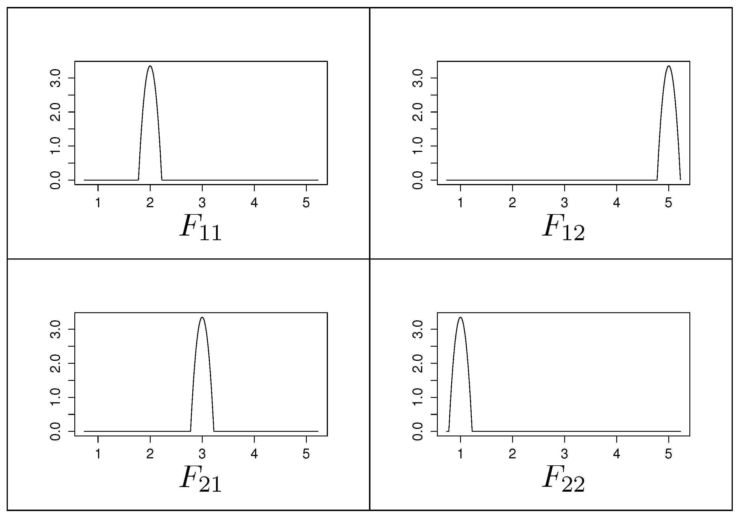
Example 2 (FP not converging to an equilibrium, although the game is zero sum [
23])
. Let the expected payoffs in a hypothetical -game be given asand let us assume that uncertainty is to be included here by allowing a bounded random deviation from these means. This variation is describable in various ways, but let us assume that the modeler has collected empirical data to construct a non-parametric estimator using Epanechnikov kernelsand replaces the entry by the distribution with mean and some small variance.The respective game with distributions as payoffs thus is again a -matrix, but with probability density functions in the cells; see Figure 1. It is easy to compute the Nash equilibrium for the exact matrix as , obtained by the mixed equilibrium strategies and for both players. Since our setting shall merely capture our uncertainty about the payoffs, we would thus naturally expect a somewhat similar result when working on the payoff distributions in Figure 1. Unfortunately, however, running FP according to the algorithm from Appendix C demonstrably fails. After a few iterations, the algorithm gets stuck in always choosing the first row for player 1, since is always -preferable over , which is immediately obvious from plotting the two distributions: Observe that choosing the upper row in the payoff structure adds probability mass to lower damages, but leaves the tail of the distribution unchanged. Thus, although the overall damage accumulates, this effect is not noticeable by the stochastic ordering based on the hyperreal relation. Consequently, the algorithm will counter-intuitively come to the conclusion that is a pure equilibrium, which is not plausible or meaningful.
Where does the process fail? The answer is found by a deeper inspection of Robinson’s proof [
24], bearing in mind that all variables are to be taken as hyperreals. The sequence enters an
-neighborhood for
once the iteration count exceeds the lower bound
, where
is the maximum (hyperreal) absolute value of the entries in the payoff matrix. Since this matrix contains all distributions, the respective
k-th order moment sequences diverge towards infinity. Hence,
is an infinitely large hyperreal, making
itself infinitely large. Hence, no iteration counter from within
can ever exceed
, which rules out convergence towards a Nash equilibrium for any algorithm running on a conventional computer, although the sequence would converge if it runs towards hyperreal infinity.
However, if we assume that the distributions all have a common support, i.e., there are no regions with zero probability mass over a whole interval
, then the individual preferences will depend on the values that the density functions in
take on at
. That is, if the matrix
is composed from all densities, then running FP boils down to running the iteration on the real-valued matrix
. The game remains zero sum, and hence the process
does converge according to [
24].
What we have discovered is thus a slightly unexpected case of a sequence (of hyperreal numbers) that is convergent, but nonetheless admits subsequences that do not converge to the limit. Based on the example from
Section 3, we may not reliably claim that the limit to which FP converges for a distribution-valued game is a Nash equilibrium, but we can identify it as a lexicographic Nash equilibrium by looking at what the process of online learning does in more detail.
4.2. Online Learning Lexicographic Nash Equilibria in Zero-Sum Games
Without loss of generality, let us consider an arbitrary payoff distribution to be represented as a vector of values , which are either direct probability masses for a categorical distribution (see criterion C1 above) or otherwise representative values computable for a continuous distribution (see criterion C2 above). So, the payoff matrix for a game with payoffs represented as full probability distributions is a matrix of vectors , and in which the payoffs are strictly ordered lexicographically.
The matrix of vectors translates into a total of d real-valued matrices, just as in the setting just described, only that the projected matrices corresponding to the respective -th coordinates of the probability mass vectors appear in reverse order of priority (so that is the matrix of all tail masses for each strategy combination , is the matrix of masses for each strategy combination, and so on). Letting the players be minimizers, they will, among two choices, prefer the distribution with less tail mass. This means nothing other than letting the FP process initially run on the matrix of last coordinates only, and from there, it will converge to a best reply. Once FP has converged, it will continue by changing strategies again to optimize the value on the second-largest coordinate. However, exactly this update forces the algorithm to then return to the last coordinate again and restore the optimum there. Here, we have another explanation as to why FP cannot converge over a countable sequence of iterations, since it would take a theoretical infinitude of steps to optimize the last coordinate, followed by a single optimization step on the second-to-last coordinate, and then taking the next infinitude of steps to restore optimality on the last coordinate again. Fortunately, we can prevent the computation from having to re-optimize over and over again, if we compute the equilibrium using plain linear programming first, and then add the constraint of not losing the optimal gains on the previous coordinate when moving to the optimization of the next coordinate.
4.3. Exact Computation of Lexicographic Nash Equilibria in Two-Player Zero-Sum Games
We can directly translate (
11) into a series of optimization problems, with more and more constraints being added: initially, on the first coordinate, we just set up a standard linear program,
in which the symbol
denotes the
-th entry of the payoff matrix
. To showcase how to proceed to the next coordinate, let us simplify and thereby better distinguish the payoff matrices by putting
and writing
, to mean the most important (matrix
of tail masses
) and second-most important payoff (
of probability masses
).
A more compact version of (LP) in matrix form, using the symbols
to denote
-matrix of all 1 s, is
where we added the subscript “1” as a reminder that
is the saddle-point payoff in the (most important) coordinate, and attained by playing the strategy
. This corresponds to solving the “
”-case of (
11).
Next, we go for the second (butlast) coordinate with payoff structure . We end up with the same linear programming problem (LP) as above, but in addition, the strategy computed in this new LP should, on the payoff structure , perform at least as well as so far, meaning that we want all coordinates of .
Intuitively, any behavior different from
would end up with a possibility for the opponent to cause less revenue than
for the first player by the equilibrium property (
5), meaning that
, since player 1 is a minimizer.
So, among the remaining equilibria, we would pick one that optimizes the second-to-last coordinate, while it retains the performance in the coordinate(s) that we had so far. This solves the “
”-case of (
11) if player 1 adds the constraint
for
, in which
is the
i-th unit vector, to the program. The next linear program that player 1 solves is thus
where, likewise, we have the saddle point
on the second coordinate, by playing strategy
, which remains optimal for the first game due to
giving at most the value
whatever player 2 does on its
m column strategies. Observe that the goals (
16) and (
17) are only different in terms of the index, which we can safely drop in an implementation; the only change relates to the constraint matrix that grows by yet another block
upon moving to the
i-th coordinate for
. The additional lines in (18) thus implement the condition to optimize over
in (
11).
Each of these linear programs remains feasible, since the first solution
is trivially feasible for (18), and so on, so that we will finally obtain an optimum
as one part of the fixed point that Proposition 2 guarantees. The complementary other part
is obtained by solving the sequence of dual programs to (
16) and (
17). Along these lines, we obtain a sequence of saddle point values
that are best accomplished under the assumption that player 2 will adapt to a change in behavior observed for player 1. This adaptation is reflected by letting player 1 anticipate it and hence add the constraint to retain its so-far-accomplished saddle point payoffs, appearing as the added constraint in (
17). Without this constraint, player 1 would simply run another equilibrium computation on the second coordinate, but just as
Section 3 has shown, player 2 can then adapt to it, and reduce the payoffs for player 1 in the first game on
. This possibility is removed by the added constraint in (
17).
This process has been practically implemented in a package for R [
44]. Concerning the complexity, the repeated linear programming has, using interior point methods, an overall polynomial complexity in the size of the game and number of dimensions to optimize. On the contrary, fictitious play has worse complexity than in the classical case (where it is worst-case exponential already), but may take even longer if the process is played over vectors or distributions. For this reason, the practical recommendation and implementation is using linear programming in the finite case.
Remark 3. Reference [37] has defined a lexicographic Nash equilibrium as a situation in which an unilateral deviation of player 1 will enable player 2 to adapt to this, and reduce player 1’s revenue accordingly. Prior work has not explained why this can be called an “equilibrium”, since the typical definition of a Nash equilibrium assumes unilateral deviations to be not responded to, i.e., the optimum holds given that all other players keep their strategies (even if mixed) unaltered. In Proposition 2, we have provided an alternative fixed-point characterization of a lexicographic Nash equilibrium, which we believe better justifies the naming as “equilibrium” in the sense of a best reply for all players, than [37] does. 


