Abstract
Multi-player mean-payoff games are a natural formalism for modelling the behaviour of concurrent and multi-agent systems with self-interested players. Players in such a game traverse a graph, while attempting to maximise a (mean-)payoff function that depends on the play generated. As with all games, the equilibria that could arise may have undesirable properties. However, as system designers, we typically wish to ensure that equilibria in such systems correspond to desirable system behaviours, for example, satisfying certain safety or liveness properties. One natural way to do this would be to specify such desirable properties using temporal logic. Unfortunately, the use of temporal logic specifications causes game theoretic verification problems to have very high computational complexity. To address this issue, we consider -regular specifications. These offer a concise and intuitive way of specifying system behaviours with a comparatively low computational overhead. The main results of this work are characterisation and complexity bounds for the problem of determining if there are equilibria that satisfy a given -regular specification in a multi-player mean-payoff game in a number of computationally relevant game-theoretic settings.
1. Introduction
Modelling concurrent and multi-agent systems such as games in which players interact by taking actions in pursuit of their preferences is an increasingly common approach in both formal verification and artificial intelligence [1,2,3]. One widely adopted semantic framework for modelling such systems is that of concurrent game structures [1]. Such structures capture the dynamics of a system—the actions that agents/players can perform, and the effects of these actions. On top of this framework, we can introduce additional structure to represent each player’s preferences over the possible paths of the system. Several approaches have been proposed for this purpose. One very natural method involves assigning a weight to every state of the game, and then considering each player’s mean-payoff over generated paths: a player prefers paths that maximise their mean-payoff [4,5,6]. These games are effective in modelling resource-bounded reactive systems, as well as any scenario with multiple agents and quantitative features. Under the assumption that each agent in the system is acting rationally, concepts from game theory offer a natural framework for understanding its possible behaviours [7]. This approach is (relatively) computationally tractable [5], expressive enough to capture applications of interest, and has been receiving increasing attention recently [8]. As such, equilibria for multi-player games with mean-payoff objectives have been studied, and the computation of Nash equilibria in such games shown to be NP-complete [5].
However, it is well-known in the game theory literature that equilibria may have undesirable properties. In the context of our setting, for example, an equilibrium may visit dangerous system states, or lead to a deadlock. Thus, one may also want to check if there exist equilibria which satisfy some additional desirable computational properties associated with the game. This decision problem—that is, determining whether a given formal specification is satisfied on some (or every) equilibrium of a given multi-agent system modelled as a multi-player game—is known as Rational Verification [9,10].
Previous approaches to rational verification have borrowed their methodology from temporal logic model checking, appealing to logics such as Linear Temporal Logic (LTL) [11] and Computation Tree Logic (CTL) [12]. However, since rational verification subsumes automated synthesis, the use of temporal logic specifications introduces high computational complexity [13]. To mitigate this problem, one might use fragments of temporal logic with lower complexity (e.g., GR(1) (generalised Reactivity(1)) formulae [14,15]), but in this work we adopt a different approach. Taking inspiration from automata theory, and in particular from [16], we consider system specifications given by a formal language for expressing ω-regular specifications, defined in terms of those states in the system that are visited infinitely often. With this approach, the complexity of the main game-theoretic decision problems is considerably lower than is the case with temporal logic specifications.
In this paper, we offer the following main contributions. We begin by introducing a language for -regular specifications and demonstrate that they form a natural construct for representing properties of concurrent games. In Section 3, we study multi-player mean-payoff games with -regular specifications in the non-cooperative setting [7], and consider the natural decision problems relating to these games and their Nash equilibria. Following this, in Section 4 we consider a cooperative solution concept derived from the core [7,17]. Finally, in Section 5 we look at reactive module games [18] as a way of succinctly representing systems, and investigate how the use of this representation affects our complexity results. We conclude with a discussion of related work in Section 6, before offering a glossary of terms, acronyms and notation used within the paper.
2. Models, Games, and Specifications
2.1. Games
A concurrent game structure [1] is a tuple,
where,
- Ag and St are finite, non-empty sets of agents and system states, respectively, where is an initial state;
- For each , is a set of actions available to agent i;
- is a transition function.
We define the size of M to be .
Concurrent games are played as follows. The game begins in state , and each player simultaneously picks an action . The game then transitions to a new state, , and this process repeats. Thus, the nth state visited is . Since the transition function is deterministic, a play of a game will be an infinite sequence of states, . We call such a sequence of states a path. Typically, we index paths with square brackets, i.e., the kth state visited in the path is denoted , and we also use slice notation to denote prefix, suffixes and fragments of paths. That is, we use to mean , for and for . Now, consider a path . We say that visits a state s if there is some such that . Since there are only finitely many states, some must be visited infinitely often. Furthermore, unless all states are visited infinitely often, there will also exist some set of states that are visited only finitely often. Thus, given a path , we can define the following two sets, which one can use to define objectives over paths: and its complement .
2.2. Strategies
In order to describe how each player plays the game, we need to introduce the concept of a strategy. Mathematically, a strategy for a given player i can be understood as a function, , which maps sequences, or histories, of states into a chosen action for player i. A strategy profile is a vector of strategies, , one for each player. The set of strategies for a given player i is denoted by and the set of strategy profiles is denoted by . If we have a strategy profile , we use the notation to denote the vector and to denote . Finally, we write as shorthand for . All of these notations can also be generalised in the obvious way to coalitions of agents, . A strategy profile together with a state s will induce a unique path, which, with a small abuse of notation, we will denote by , as well as an infinite sequence of actions , with . These paths are obtained in the following way. Starting from s, each player plays . This transforms the game into a new state, given by . Each player then plays , and this process repeats infinitely often. Typically, we are interested in paths that begin in the game’s start state, , and we write as shorthand for the infinite path .
When considering computational questions surrounding concurrent games, it is useful to work with a finite representation of strategies. We use two such representations: finite-memory strategies and memoryless strategies. A finite-memory strategy is a finite state machine with output: for player i, a finite-memory strategy is a four-tuple, , where is a finite, non-empty set of internal states with an initial state, is an internal transition function and is an action function. This strategy operates by starting in the initial state, and for each state it is in, producing an action according to , looking at what actions have been taken by everyone, and then moving to a new internal state as prescribed by . Now, it is not hard to see that, if we have multiple finite-memory strategies playing against each other, then the play they generate will be periodic: the play must eventually revisit some configuration, and at this point, the game will start to repeat itself. More precisely, any play generated by a collection of finite-memory strategies will consist of a finite non-repeating sequence of states, followed by a finite sequence that repeats infinitely often. Because such a play will be periodic, we can write the path induced on the concurrent game structure as , for some with .
Finally, a memoryless strategy is a strategy that depends only on the state the player is currently in. Thus, memoryless strategies can be expressed as functions , which simply map states to actions; such functions can be directly implemented as lookup tables, in space . Note that memoryless strategies can be encoded as finite-memory strategies, and that finite-memory strategies are a special case of arbitrary strategies . Whilst we will work with finite-memory and memoryless strategies, we will use arbitrary strategies by default, unless otherwise stated.
2.3. Mean-Payoff Games
A two-player, mean-payoff game [4,6], is defined by a tuple:
Here and are disjoint, with . Additionally, we have: and w is a function with signature . There are two players, 1 and 2, and the vertices in should be thought of as those that player i controls—informally, the players take turns choosing edges to traverse, each of which is weighted. Player 1 is trying to maximise the average of the weights encountered, whilst player 2 is trying to minimise it. Formally, the game begins in state and player 1 chooses an edge . Then player 2 chooses an edge and this process repeats indefinitely. This induces a sequence of weights, , and player 1 (respectively, 2) chooses edges to try and maximise (respectively, minimise) the mean-payoff of , denoted , where for , we have:
There are two keys facts about two-player, mean-payoff games that we shall use without comment throughout. The first is that memoryless strategies suffice for both players to act optimally (i.e., achieve their maximum payoff) [4]. The second is that every game has a value (i.e., a payoff that player 1 can achieve regardless of what player 2 plays) and determining if a game’s value is equal to v lies in [6]. In particular, given a game, determining its value can be seen as a problem that lies within TFNP [19].
Extending two-player, mean-payoff games to multiple players, a multi-player mean-payoff game [5] is given by a tuple,
where M is a concurrent game structure and for each agent , is a weight function. In a multi-player mean-payoff game, a path induces an infinite sequence of weights for each player, We denote this sequence by . Under a given path, , a player’s payoff is given by . For notational convenience, we will write for . We can then define a preference relation over paths for each player as follows: . We also write if and not . Note that, since strategy profiles induce unique plays , we can lift preference relations from plays to strategy profiles, for example writing as a shorthand for .
In what follows, we refer to multi-player, mean-payoff games simply as mean-payoff games, and refer to two-player, mean-payoff games explicitly as such.
2.4. Solution Concepts
To analyse our games, we make use of solution concepts from both the non-cooperative and cooperative game theory literatures. With respect to non-cooperative solution concepts, a strategy profile is said to be a Nash equilibrium [20,21] if for all players i and strategies , we have . Informally, a Nash equilibrium is a strategy profile from which no player has any incentive to unilaterally deviate. In addition to Nash equilibrium, we also consider the cooperative solution concept known as the core [17,22]. While Nash equilibria are profiles that are resistant to unilateral deviations, the core consists of profiles that are resistant to those deviations by coalitions of agents, where every member of the coalition is better off, regardless of what the rest of the agents do. Formally, we say that a strategy profile, , is in the core if for all coalitions , and strategy vectors , then there is some complementary strategy vector such that , for some . Given a game G, let denote the set of Nash equilibrium strategy profiles of G, and let denote the set of strategy profiles in the core of G.
It is worth noting that if a strategy profile is not a Nash equilibrium, then at least one player can deviate and be better off, under the assumption that the remainder of the players do not change their actions. However, if a strategy profile is not in the core, then some coalition can deviate and become better off, regardless of what the other players do. Thus, the core should not be confused with the solution concept of strong Nash equilibrium: a strategy profile that is stable under multilateral deviations, assuming the remainder of the players ‘stay put’ [23,24]. We will not use strong Nash equilibria in this work, and only mention the concept in order to emphasise how strong Nash equilibria are different from the core.
2.5. -Regular Specifications
In [16], Boolean combinations of atoms of the form are used to describe acceptance conditions of arbitrary -automata. We use this approach to specify system properties for our games. Formally, the language of -regular specifications, , is defined by the following grammar:
where F ranges over subsets of St. For notational convenience, we write as shorthand for , for and we define disjunction, , implication and bi-implication in the usual way. The size of a specification is simply the sum of the sizes of the sets within its atoms. We now talk about what it means for a path to model a specification. Let be a path, F be a subset of St and be arbitrary -regular specifications. Then,
- , if ;
- , if it is not the case that ;
- , if both and .
Note that we use Inf in two different, but interrelated senses. First, we use it as an operator over paths, as in , to denote the set of states visited infinitely often in a path , but we also use it as an operator over sets, as in , as an atom in the specifications just defined. The semantics of the latter are defined in terms of the former. We will use these interchangeably: usage will be clear from the context. Using this notation, we can readily define conventional -regular winning conditions, as follows:
| Type | Associated Sets | -Regular Specification |
| Büchi | ||
| Co-Büchi | ||
| Gen. Büchi | ||
| Rabin | ||
| Streett | ||
| Muller |
Our -regular specifications are equivalent to Emerson-Lei conditions [25], albeit with a different syntax. We can in fact represent all possible -regular winning conditions—as another example, consider parity conditions. Suppose each state is labelled by a function, , with for some , for all . Given a path, , the traditional parity condition is satisfied when is odd. The sets of interest are defined by:
Then, assuming m is odd (the formula for m even is similar), the parity condition can be expressed by the following specification:
With -regular specifications defined, we can talk about them in the context of games. Let be some strategy profile. Then, induces some path, , and given that -regular specifications are defined on paths, we can talk about paths induced by strategies modelling specifications. However, we are not interested in whether the paths induced by arbitrary strategies model a given specification—it is more natural in the context of multi-player games to ask whether the paths induced by some or all of the equilibria of a game model a specification, both in the non-cooperative and in the cooperative contexts. In particular, we are interested in the Nash equilibria and the core, and whether the paths induced by strategy profiles that form an instance of these solution concepts model a specification.
Example 1.
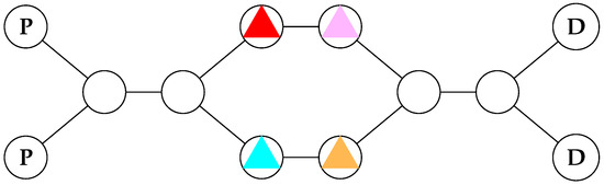
Suppose we have four delivery robots in a warehouse (given by the coloured triangles in Figure 1), who want to pick up parcels at the pickup points (labelled by the bold Ps) and drop them off at the delivery points (labelled by the bold Ds). If a robot is not holding a parcel, and goes to a pickup point, it automatically gets given one. If it has a parcel, and goes to the delivery point, then it loses the parcel, and gains a payoff of 1. Furthermore, if two robots collide, by entering the same node at the same time, then they crash, and get a payoff of at every future timestep.
Figure 1.
Robots manoeuvering in a warehouse.
Now, there are a number of Nash equilibria here (infinitely many, in fact), but it is easy to see that many of them exhibit undesirable properties. For instance, consider the strategy profile where red and pink go back and forth between the pickup and delivery points, and threaten to crash into, or deadlock, blue and yellow if they move from their starting positions. This is a Nash equilibrium, but is clearly not Pareto optimal—a socially undesirable outcome.
It is easy to identify the most socially desirable outcome—all four robots visiting the pickup and delivery points infinitely often, waiting for the others to pass when they reach bottleneck points. If we call the set containing the two states where robot i visits a pickup point and similarly label the set of delivery points , we can express this condition concisely with the following ω-regular specification:
Thus, we can conclude that there exists some Nash equilibrium which models the above (Generalised Büchi) specification. However, we just did this by inspection. In practice, we would like to ask this question in a more principled way. As such, we will spend the rest of this paper exploring the natural decision problems associated with mean-payoff games with ω-regular specifications.
2.6. Mean-Payoff Games with -Regular Specifications
Given that we have proposed -regular specifications as an alternative to LTL [11] specifications, it is natural to ask how they compare. The connection between them is given by the following statement:
Proposition 1.
Let G be a game and let α be some ω-regular specification. Then there exists a set of atomic propositions, Φ, a labelling function , and an LTL formula φ such that, for all paths π, we have if and only if .
Proof.
Without loss of generality, we may assume that is written in conjunctive normal form, that is:
where each is an atom of the form or for some subset . We start by introducing a propositional variable for every subset . Then, for a given state , we define:
Then, we simply define:
where if and if . We claim that for all paths , we have if and only if .
First suppose that . Thus, by definition, we have for all that . This in turn implies that there exists some j such that . If , then this implies that . Take any . By definition, we have and so we also have . However, by construction, this implies .
Similarly, if , then we have . Thus, for all , we have and so we have . By construction, this implies that . Thus, for all i, there exists some j such that . This implies that .
Conversely, suppose that . So for all i, there exists a j such that . If , then visits some state infinitely often. Thus, , so . Similarly, if , then . Either way, we have . So for all i, there exists some j such that , implying that . □
Thus, -regular specifications can be seen as being ‘isomorphic’ to a strict subset of LTL (it is straightforward to come up with LTL formulae that cannot be written as -regular specifications—take for instance , where is some non-trivial propositional formula). As such, we hope the restriction of the setting may yield some lower complexities when considering the analogous decision problems. That is, we will study a number of decision problems within the rational verification framework [10,17], where -regular specifications replace LTL specifications in a very natural way.
Firstly, given a game, a strategy profile, and an -regular specification, we can ask if the strategy profile is an equilibrium whose induced path models the specification. Secondly, given a game and an -regular specification, we can ask if the specification is modelled by the path/paths induced by some/every strategy profile in the set of equilibria of the game. Each of these problems can be phrased in the context of a non-cooperative game or a cooperative game, depending on whether we let the set of equilibria be, respectively, the Nash equilibria or the core of the game. Formally, in the non-cooperative case, we have the following decision problems:
MEMBERSHIP:
Given: Game G, strategy profile , and specification, .
Question: Is it the case that and ?
E-NASH:
Given: Game G and specification .
Question: Does there exist a such that ?
A natural dual to E-NASH is the A-NASH problem, which instead of asking if the specification holds in the path induced by some Nash equilibrium, asks if the specification holds in all equilibria:
A-NASH:
Given: Game G and specification .
Question: Is it the case that , for all ?
These decision problems were first studied in the context of iterated Boolean games [26], and are the ‘flagship‘ decision problems of rational verification [18].
In the cooperative setting, the analogous decision problems are defined by substituting for . We refer to these problems as MEMBERSHIP, E-CORE, and A-CORE, respectively, (with a small abuse of notation for the first problem: context will make it clear whether we are referring to the non-cooperative or cooperative problem). These variants were first studied in the setting of LTL games [17].
It is worth noting here one technical detail about representations. In the E-NASH problem, the quantifier asks if there exists a Nash equilibrium which models the specification. This quantification ranges over all possible Nash equilibria and the strategies may be arbitrary strategies. However, in the MEMBERSHIP problem, the strategy is part of the input, and thus, needs to be finitely representable. Therefore, when considering E-NASH (or A-NASH, or the corresponding problems for the core), we place no restrictions on the strategies, but when reasoning about MEMBERSHIP, we work exclusively with memoryless or finite-memory strategies.
Before we proceed to studying all these problems in detail, we note that even though some other types of games (for example, two-player, turn-based, zero-sum mean-payoff, or parity games) can be solved only using memoryless strategies, this is not the case in our setting:
Proposition 2.
There exist games G and ω-regular specifications α such that for some Nash equilibrium , but for which there exists no memoryless Nash equilibrium such that . The statement also holds true for the core.
Proof.
and the weight functions for the players defined as,
Consider the game, , where is defined as follows: , , , with the transition relation defined to be,
| Ac | |||||
| St | |||||
| mid | right | mid | mid | left | |
| right | right | mid | mid | mid | |
| left | mid | mid | mid | left | |
| 1 | 2 | |
| mid | 0 | 0 |
| right | 1 | 0 |
| left | 0 | 1 |
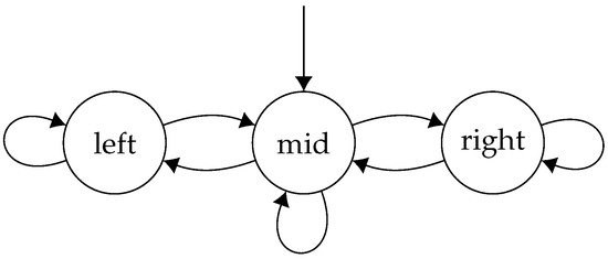
Thus, the game looks like the following concurrent game structure (Figure 2):
Figure 2.
A game where a finite-memory Nash equilibrium is required to model an -regular specification.
In this game, each player decides whether they want to go left or right. When they both agree on what direction they want to go, they move in that direction. If they disagree, then they end up in the middle state. We now produce a finite memory strategy profile, , and a specification such that is a Nash equilibrium and . The basic idea is that with finite memory strategies, the two players can alternate between the left and right state, each achieving a strictly positive payoff, threatening to punish one another if either deviates from this arrangement, whilst this is not possible in memoryless strategies, as in this case the players would have to take the same action each time in the middle state.
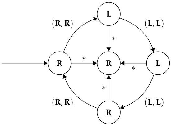
Consider the following strategy, , for player 1 (Figure 3):
Figure 3.
A finite memory strategy for player 1 which forms part of a Nash equilibrium which models the given specification. The asterisks * are wildcards—they match any action which isn’t explicitly detailed on the diagram.
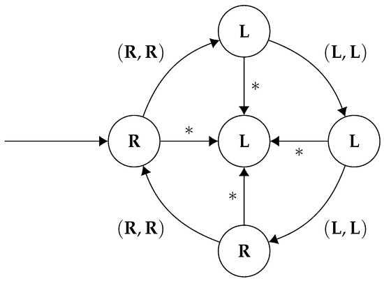
Furthermore, the corresponding strategy, for player 2 (Figure 4):
Figure 4.
A finite memory strategy for player 2 which forms part of a Nash equilibrium which models the given specification. The asterisks * are wildcards—they match any action which isn’t explicitly detailed on the diagram.
It is easy to verify that is a Nash equilibrium. Each player gets a mean payoff of under . Suppose player 1 deviates to another strategy, which does not match the sequence of actions as dictated by . Then player 2 will just start playing forever, meaning that the game will never enter the right state again, implying player 1 gets a payoff of zero. By symmetry, we can conclude that this is a Nash equilibrium. Moreover, letting be the -regular specification , we see that .
However, note that there cannot exist a memoryless Nash equilibrium, , such that . In a memoryless strategy, for a given state, both players must commit to an action and only play that given action vector in that state. If both players play in the middle state, then they will never be able to reach the left state, and if they both play in the middle state, they will never reach the right state. Additionally, if they disagree, then they will perpetually stay in the middle state. Thus, there cannot exist a memoryless strategy profile , such that . This example demonstrates that, in general, memoryless strategies are not powerful enough for our games: there may exist a Nash equilibrium which satisfies the specification, with no memoryless Nash equilibrium which satisfies it. Finally, note that is also in the core—individual deviations have been already accounted for, and clearly no group deviation containing both players strictly improves both pay-offs. □
3. Non-Cooperative Games
In the non-cooperative setting, MEMBERSHIP, E-NASH, and A-NASH are the relevant decision problems. In this section, we will show that MEMBERSHIP lies in P for memoryless strategies, while E-NASH is NP-complete and even remains NP-hard when restricted to memoryless strategies—thus, no worse than solving a multi-player mean-payoff game [5]. Because A-NASH is the dual problem of E-NASH, it follows that A-NASH is co-NP-complete. In order to obtain some of these results, we also provide a semantic characterisation of the paths associated with strategy profiles in the set of Nash equilibria that satisfy a given -regular specification. We will first study the MEMBERSHIP problem, and then investigate E-NASH, providing an upper bound for arbitrary strategies and a lower bound for memoryless strategies—arguably, the simplest, yet still computationally important, model of strategies one may want to consider for multi-agent systems.
Theorem 1.
For memoryless strategies, MEMBERSHIPis in P.
Proof.
We verify that a given strategy profile is a Nash equilibrium in the following way. We begin by calculating the payoff of each player in the strategy profile by ‘running’ the strategy and keeping note of the game states. When we encounter the same game state twice, we can simply take the average of the weights encountered at the states between the two occurrences, and that will be the payoff for a given player. By the pidgeonhole principle, it will take no more than time steps to get to this point, and thus, this can be done in linear time.
Once we have each player’s payoff, we can determine if they have any incentive to deviate in the following way—for each player, look at the graph induced by the strategy profile excluding them. Formally, the graph induced by a partial strategy profile , denoted by is defined as follows: the set of nodes, V, simply consists of the set of states of the game, that is, and the set of edges are simply the moves available to player i—that is, if , then there exists some such that .
We can use Karp’s algorithm [27] to determine the maximum payoff that this player can achieve given the other players’ strategies. If this payoff is higher than the payoff originally achieved, then this means player i can successfully deviate from the given strategy profile and be better off, and so it is not a Nash equilibrium. If we do this for each player, and the maximum payoff each player can achieve to equal to their payoff in the given strategy profile, then we can conclude it is a Nash equilibrium, and moreover, we have determined this in polynomial time.
To determine if the strategy profile satisfies the specification, we run the strategy as before, and determine the periodic path which the game will end up in. This tells us which states will be finitely and infinitely visited, which in turn induces a valuation which will either model or not model the specification. Checking this can be done in polynomial time and thus, we can conclude that for memoryless strategies, MEMBERSHIP lies in P. □
The simplicity of the above algorithm may raises hopes that it might extend to finite-memory strategies. However, in this case, the configuration of the game is not just given by the current state—it is given by the current state, as well as the state that each of the player’s strategies are in. Thus, we might have to visit at least (where Q is the smallest set of strategy states over the set of players) configurations until we discover a loop. Now whilst there is an exponential dependency on the number of players in the input to the problem, this bound on the number of configurations is not necessarily polynomial in the size of the input. More precisely, the size of the underlying concurrent game structure is and so if is larger that , the number of configurations will grow exponentially faster than the size of the input. Thus, we cannot use the above algorithm in the case of finite memory strategies to get a polynomial time upper bound.
We now consider the E-NASH problem. Instead of providing the full NP-completeness result here, we start by showing that the problem is NP-hard, even for memoryless strategies, and delay the proof of the upper bound until we develop a useful characterisation of Nash equilibrium in the context of -regular specifications. For now, we have the following hardness result, obtained using a reduction from the Hamiltonian cycle problem [28,29]—a similar, but simpler, argument can be found in [5].
Proposition 3.
E-NASHis NP-hard, even for games with one player, constant weights, and memoryless strategies.
Proof.
Let be a graph with . We form a mean-payoff game G by letting and . We pick the initial state arbitrary and label it , and the actions for player 1 correspond to the edges of G. That is, we have and we have if and only if . Finally, we fix an integer constant and let for all .
Let for each and let be the following specification:
We claim that G has a Hamiltonian cycle if and only if G has a memoryless Nash equilibrium such that .
First suppose that G has a Hamiltonian cycle, . We define a memoryless strategy, , for player 1 by setting , where the superscript is interpreted modulo n. As is a Hamiltonian cycle, it visits every node, so is a well-defined, total function. By definition, we see that , so we have . Additionally, as each state has the same payoff, this strategy is trivially a Nash equilibrium.
Now suppose that G has a memoryless Nash equilibrium such that . Let . Since is memoryless, must be of the form for integers i and j. Without loss of generality, assume that i and j are the smallest integers such that this holds. Moreover, since , the path visits every state infinitely often so we must have that contains every state, and by memorylessness, it must be a cycle. Thus, by definition, is a Hamiltonian cycle. □
Theorem 1 and Proposition 3 together establish NP-completeness for multi-player mean-payoff games with -regular specifications and memoryless strategies: one can non-deterministically guess a memoryless strategy for each player (which is simply a list of actions for each player, one for each state), and use MEMBERSHIP to verify that it is indeed a Nash equilibrium that models the specification. However, as we shall show later, the problem is also NP-complete in the general case. To prove this, we need to develop an alternative characterisation of Nash equilibria.
To do this, we need to introduce the notion of the punishment value in a multi-player mean-payoff game; cf., [30,31]. The punishment value, , of a player i in a given state s can be thought of as the worst value the other players can impose on a player at a given state. Concretely, if we regard the game G as a two player, zero-sum game, where player i plays against the coalition , then the punishment value for player i is the smallest mean-payoff value that the rest of players in Ag can inflict on i from a given state. Formally, given a player i and a state , we define the punishment value, against player i at state s, as follows:
How efficiently can we calculate this value? As established in [5], we proceed in the following way: in a two player, turn-based, zero-sum, mean-payoff game, positional strategies suffice to achieve the punishment value [4]. Thus, we can non-deterministically guess a pair of positional strategies for each player (one for the coalition punishing the player, and one for the player themselves), use Karp’s algorithm [27] to find the maximum payoff for both the player and the coalition against their respective punishing strategies, and then verify that the two values coincide. With this established, we have the following lemma, which can be proved using techniques for mean-payoff games adapted from [5,15].
Lemma 1.
Let π be a path in G and let be the path of associated action profiles. Then there is a Nash equilibrium, , such that if and only if there exists some , with , such that:
- for each k, we have for all and , and;
- for all players , we have .
Proof.
First assume that we have some Nash equilibrium such that . Suppose there does not exist any with the desired properties. Furthermore, let us first suppose that for all , with , there exists some player such that . However, this is true for all . So we have . This means that player i might as well play the positional strategy which ensures they achieve at least the punishment value. This in turn means that player i has some deviation, contradicting the fact that is a Nash equilibrium.
So instead, it must be the case that for all , with , there is some time step k, a player i and an action such that . However, since this is true for all , it is true for . Furthermore, since , this gives a contradiction—we cannot have . Thus, it follows that the first part of the statement is true.
Now assume that there exists some with the properties as prescribed in the statement of the lemma. We define a strategy profile in the following way. Each player follows . If any player chooses to deviate from , say at state , with an action then the remaining players play the punishing strategy which causes player i to have a payoff of at most . Thus, no player has any incentive to deviate away from and so we have a Nash equilibrium with . □
With this lemma in mind, we define a graph, as follows. We set and include if there exists some action profile such that with for all and . Having done this, we then prune any components which cannot be reached from the start state and then remove all states and edges not contained in F, before reintroducing any states in F that may have been removed. Thus, given this definition and the preceding lemma, to determine if there exists a Nash equilibrium which satisfies an -regular specification, , we calculate the punishment values, and guess a vector , as well a set of states, F, which satisfy the specification. Letting , we form the graph and then check if there is some path in with for each player i which visits every state infinitely often. Trivially, if this graph is not strongly connected, then no path can visit every state infinitely often. Thus, to determine if the above condition holds, we need one more piece of technical machinery, in the form of the following proposition:
Proposition 4.
Let be a strongly connected graph, let be a set of weight functions, and let . Then, we can determine if there is some path π with the properties,
- π visits every state infinitely often;
- for each ,
in polynomial time.
Conceptually, Proposition 4 is similar to Theorem 18 of [5], but with two key differences—firstly, we need to do additional work to determine if there is a path that visits every state infinitely often. Moreover, the argument of [5] is adapted so we have the corollary that if there is a Nash equilibrium that models the specification, then there is some finite state Nash equilibrium that also models the specification. This means that the construction in our proof can be used not only for verification, but also for synthesis.
For clarity of presentation, we shall split the above proposition into two constituent lemmas. To do this, we begin by defining a system of linear inequalities. We then go on to show that there is a path with the desired properties if and only if this system has a solution—one lemma for each direction. As the system of inequalities can be determined in polynomial time, this yields our result.
For a graph G, a set of weight functions be a set of weight functions, and a vector , we define a system of linear inequalities, as follows: for each agent , and each edge , introduce a variable , along with the following inequalities:
- (i)
- for each agent and for each edge .
- (ii)
- for each agent .
- (iii)
- for all and for each .
- (iv)
- for all .
- (v)
- for all .
It is worth briefly discussing what this system is actually encoding. Roughly speaking, the set defines a cycle for each player that makes sure their payoff is greater than . Each represents the proportion that a given edge is visited in the cycle. The idea is that we define a path by visiting each an appropriate number of times, before travelling to the next cycle and visiting that repeatedly.
Conversely, if there exists some path with the stated properties, it will also define a solution to the system of inequalities. This has the corollary that if there is a Nash equilibrium in the game, then there is a finite state Nash equilibrium as well.
In what follows, for an edge and a weight function , we define . We also extend weight functions to finite paths in the natural way, by summing along them.
Lemma 2.
Let be a strongly connected graph, let be a set of weight functions, let . Furthermore, suppose there exists some path π such that for each , which visits every state infinitely often. Then has a solution.
Proof.
First suppose there exists some path with the stated properties. For each and , define to be the following quantity:
Informally, for a given edge e, gives us the proportion that e appears in the prefix . Note that for all and all . Additionally, for each n, it easy to see we have:
By definition, for each we have:
Thus, there must exist some subsequence of the natural numbers, , such that:
With this defined, we introduce a sequence of numbers, for each edge , by defining . Now, as is a bounded sequence, by the Bolzano-Weierstrass theorem, there must be a convergent subsequence for each edge e, . We define and claim that these form a solution to the system of inequalities.
Since , it is clear that we have . Thus, Inequality (i) is satisfied. Additionally, by Equation (2), we can deduce that for each t, and for every , we have:
Taking limits, we can conclude that Inequality (ii) is satisfied. To establish (iii), by definition of , fix a . In a path, if we enter a node, we must exit it. Thus, we have:
implying,
Taking the relevant subsequence and letting , we can deduce that Inequality (iii) is satisfied. To establish (iv), first note that for all , we have,
The equality between lines 4 and 5 is valid, as we have established that the limit exists in line 2. Thus, since we have , by assumption, we can conclude that Inequality (iv) is valid. In a similar fashion, note that for all , we have,
This, together with Inequality (iv), implies that Inequality (v) is satisfied.
Thus, putting all this together, we can conclude that if there exists some path with the stated properties, then there also exists a solution to , the system of linear inequalities. □
We now show the other direction:
Lemma 3.
Let be a strongly connected graph, let be a set of weight functions, let . Suppose that has a solution. Then there exists some path π such that for each , which visits every state infinitely often.
Proof.
Given that there is a solution to , there must exist a solution that consists of rational numbers. Thus, letting be a rational solution, we can write , for some , and some appropriately chosen .
Now, for each , we form a multigraph, , which takes G and replaces each edge e by copies. Note that whilst G is strongly connected, some of the may be equal to 0, which would mean that is disconnected.
Now, by Inequality (iii), for each , we have:
Thus, the in-degree of each vertex in is equal to its out-degree. Thus, each strongly connected component of contains an Eulerian cycle (An Eulerian cycle is a path that starts and ends at the same node which visits every edge exactly once). Interpreting each of these Eulerian cycles as paths in G, we get a set of (not necessarily simple) cycles for each agent, , where .
Now for each agent , and every , we define a cycle which starts at the first state of , traces n times, takes the shortest path from the start state of to , traces n times and repeats this process for all the cycles of agent i, until it has traced n times. From here, it then takes the shortest path to the start state of .
Let be the largest of the absolute values of the weights of agent i. That is, . Then we have for all ,
and,
Putting these together, we get:
Taking limits, we see that:
Thus, for sufficiently large, we must also have, for all :
Moreover, if is large enough, the above equation will be true for all . Assuming this is the case, we set . Then, for all , we have,
We are now ready to define a path , which will form the basis for our path of interest, . The path starts by visiting N times, before taking the shortest path to the start of , and visiting that N times, and so on. Once has been visited N times, we then take the shortest path that visits any states that have not been yet visited, before returning to the start vertex of .
Let us look at each player’s payoff on . We have:
Taking limits as before, we can conclude that for sufficiently large, we have:
We then simply define to be the path that repeatedly traverses . It is easy to see that and that visits every state infinitely often. □
We can now combine these two results to obtain our proof:
Proof.
(Proof of Proposition 4) Given the statement of the proposition, we construct an algorithm which forms the linear program and see if it has a solution. As the linear program is of polynomial size, and as linear programs can be solved in polynomial time, we see that the overall algorithm can be done in polynomial time. By Lemma 3, we see that the algorithm is sound and then by Lemma 2, we see it is complete. □
From the propositions above, we can establish the complexity of E-NASH:
Theorem 2.
E-NASHis NP-complete.
Proof.
For NP-hardness we have Proposition 3. For the upper bound, suppose we have an instance, , of the problem. Then we proceed as follows. We non-deterministically guess pairs of punishing strategy profiles, for each player , a state for each player, and a set of states F. From these, we can easily check that the valuation induced by F satisfies the specification and we can also use Karp’s algorithm to compute the punishment values, , for each state and for each player . Setting , we invoke Lemma 1 and form the graph . If it is not strongly connected, then we reject. Otherwise, we use Proposition 4 to determine if the associated linear program has a solution. If it does, then we accept, otherwise we reject. □
Another benefit of splitting Proposition 4 is that it readily yields the following corollary:
Corollary 1.
Let G be a game and α an ω-regular specification. Suppose that G has some Nash equilibrium such that . Then, G also has some finite-memory Nash equilibrium such that .
Proof.
Suppose G has some Nash equilibrium such that . Furthermore, let . Then by Lemma 1, there exists some , with , and a subset such that in , visits every state infinite often and for each , we have . By Lemma 2, we see that the system of inequalities has a solution. However, then by Lemma 3, we see that there exists some periodic path such that in , again, we have that π′ visits every state infinite often and for each , we have . Thus, applying Lemma 1 again, we see that G has some Nash equilibrium such that with . Moreover, by the construction in Lemma 3, we see that we may assume that is a finite-memory strategy. □
4. Cooperative Games
We now move on to investigate cooperative solution concepts, and in particular, the core. We start by studying the relationship between Nash equilibrium and the core in our context. We first establish that they are indeed different:
Proposition 5.
Let G be a game with . Then, . However, if , then there exist games G such that , and games G such that .
Thus, the two concepts do not coincide beyond the one-player case. In fact, there are two-player games in which the set of Nash equilibria is empty, while the core is not, which demonstrates that the core is not a refinement of Nash equilibrium. Nor does the other direction hold: Nash equilibrium is not a refinement of the core. The following two games (Figure 5 and Figure 6) serve as witnesses to these claims.
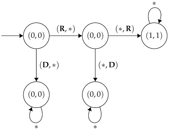
Figure 5.
. The asterisks * are wildcards—they match any action which isn’t explicitly detailed on the diagram.
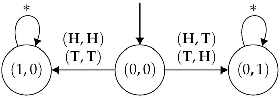
Figure 6.
. The asterisks * are wildcards—they match any action which isn’t explicitly detailed on the diagram.
As we can see in the game in Figure 5, has a Nash equilibrium that is not in the core (and in which both players get a mean-payoff of 0—cf., Player 1 choosing at the initial state while Player 2 chooses at the middle state), since the coalition containing both players has a beneficial deviation in which both players get a mean-payoff of 1. On the other hand, in the game in Figure 6, has a non-empty core (consider every possible memoryless strategy) while it has an empty set of Nash equilibria. Moreover, in both games, the detailed strategies can be implemented without memory.
Regarding memory requirements, as with Nash equilibrium, it may be that, in general, memoryless strategies are not enough to implement all equilibria in the cooperative setting. Indeed, there are games with a non-empty core in which no strategy profile in the core can be implemented in memoryless strategies only. Take, for instance, the game shown in Figure 2, with the weights changed to , . Only if the two players collaborate, and alternate between left and right, they will get their optimal mean-payoffs (of 2). Clearly, such an optimal payoff for both players cannot be obtained using only memoryless strategies.
Another important (game-theoretic) question about cooperative games is whether they have a non-empty core, a property that holds for games with LTL goals and specifications [17]. However, that is not the case for mean-payoff games, at least for games with .
Proposition 6.
In mean-payoff games, if , then the core is non-empty. For , there exist games with an empty core.
Proof.
If , because of Proposition 5, the core coincides with the set of Nash equilibria in one-player games, which is always non-empty. For two-player games, let be any strategy profile. If is not in the core, then either Player 1, or Player 2, or the coalition consisting of both players has a beneficial deviation. If the latter is true, then there is a strategy profile, such that for both . We repeat this process until the coalition of both players does not have a beneficial deviation. This must eventually be the case as each player’s payoff is capped by their maximum weight, so either they both reach their corresponding maximum weight, or there comes a point when they cannot beneficially deviate together. At this point, we must either be in the core, or either player 1 or player 2 has a beneficial deviation. If player j () has a beneficial deviation, say , then any strategy profile , with , that maximises Player i’s mean-payoff is in the core. Thus, for every two-player game, there exists some strategy profile that lies in the core.
However, for three-player mean-payoff games, in general, the core of a game may be empty. Consider the following three-player game G, where each player has two actions, , and there are four states, . The states are weighted for each player as follows:
| 1 | 2 | 3 | |
| P | |||
| R | 2 | 1 | 0 |
| B | 0 | 2 | 1 |
| Y | 1 | 0 | 2 |
If the game is in any state other than P, then no matter what set of actions is taken, the game will remain in that state. Thus, we only specify the transitions for the state P:
| Ac | St |
| R | |
| R | |
| B | |
| P | |
| P | |
| Y | |
| B | |
| Y |
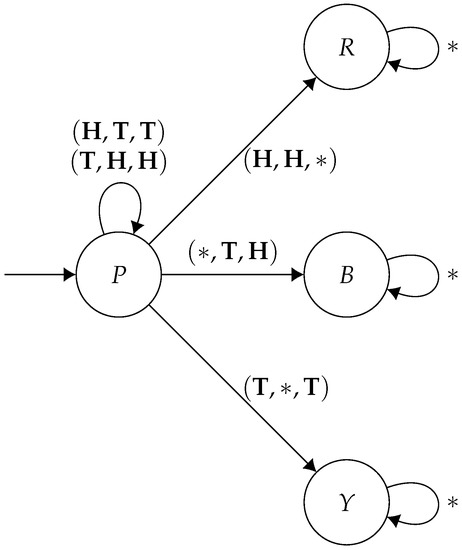
Thus, the structure of this game looks like the following graph (Figure 7):
Figure 7.
A game with an empty core. The asterisks * are wildcards—they match any action which isn’t explicitly detailed on the diagram.
Note that strategies are characterised by the state that the game eventually ends up in. If the players stay in P forever, then they can all collectively change strategy to move to one of , and each get a better payoff. Now, if the game ends up in R, then players 2 and 3 can deviate by playing , and no matter what player 1 plays, they will be in state B, and will be better off. However, similarly, if the game is in B, then players 1 and 3 can deviate by playing to enter state Y, in which they both will be better off, regardless of what player 2 does. Furthermore, finally, if in Y, then players 1 and 2 can deviate by playing to enter R and will be better off regardless of what player 3 plays. Thus, no strategy profile lies in the core. □
Before proceeding, it is worth reflecting on the definition of the core. We can redefine this solution concept in the language of ‘beneficial deviations’. That is, we say that given a game G, a strategy profile , a beneficial deviation by a coalition C, is a strategy vector such that for all complementary strategy profiles , we have for all . We can then say that is a member of the core, if there exists no coalition C which has a beneficial deviation from . Note this formulation is entirely identical to our earlier definition of the core.
From a computational perspective, there is an immediate concern here—given a potential beneficial deviation, how can we verify that it is preferable to the status quo under all possible counter-responses? Given that strategies can be arbitrary mathematical functions, how can we reason about that universal quantification effectively? Fortunately, as we show in the following lemma, we can restrict our attention to memoryless strategies when thinking about potential counter-responses to players’ deviations:
Lemma 4.
Let G be a game, be a coalition and be a strategy profile. Further suppose that is a strategy vector such that for all memoryless strategy vectors , we have:
Then, for all strategy vectors, , not necessarily memoryless, we have:
Before we prove this, we need to introduce an auxiliary concept of two-player, turn-based, zero-sum, multi-mean-payoff games [32] (we will just call these multi-mean-payoff games moving forward). Informally, these are similar to two-player, turn-based, zero-sum mean-payoff games, except player 1 has k weight functions associated with the edges, and they are trying to ensure the resulting k-vector of mean-payoffs is component-wise greater than a vector threshold. Formally, a multi-mean-payoff game is a 5-tuple, , where are sets of states controlled by players 1 and 2, respectively, with the state space, the start state, a set of edges and a weight function, assigning to each edge a vector of weights.
The game is played by starting in the start state, , and player i choosing an edge , and traversing it to the next state. From this new state, , player j chooses an edge and so on, repeating this process forever. Paths are defined in the usual way and the payoff of a path , , is simply the vector . Finally, is a threshold vector and player 1 wins if the for all , and loses otherwise. An important question associated with these games is whether player 1 can force a win. As shown in [32], this problem is co-NP-complete. Whilst we do not need to utilise this result right now, this sets us up to prove Lemma 4:
Proof.
(Proof of Lemma 4) Let be an arbitrary strategy and let be an arbitrary agent. Denote by and by . We aim to show that . Suppose instead it is the case that . Thus, we have . Considering this as a two-player multi-mean-payoff game, where player 1’s strategy is fixed and encoded into the game structure (i.e., player 1 follows , but has no say in the matter), and the payoff threshold is , then is a winning strategy for player 2 in this game. Now, by [32,33], if player 2 has a winning strategy, then they have a memoryless winning strategy. Thus, there is a memoryless strategy such that . However, this contradicts the assumptions of the lemma, and thus we must have (In [32], their winning condition relates to whether a player’s payoff is greater than or equal to a given vector. One can adapt this argument to show it is also true for strict inequalities). □
We now look at some complexity bounds for mean-payoff games in the cooperative setting. Having introduced beneficial deviations, let us consider the following decision problem:
BENEFICIAL-DEVIATION (BEN-DEV):
Given: Game G and strategy profile .
Question: Is there and such that for all and for all , we have:
Using this new problem, we can prove the following statement:
Proposition 7.
Let G be a game, a strategy profile, and α a specification. Then, if and only if and .
Proof.
Proof follows directly from definitions. □
The above proposition characterises the MEMBERSHIP problem for cooperative games in terms of beneficial deviations, and, in turn, provides a direct way to study its complexity. In the remainder of this section we concentrate on the memoryless case.
Theorem 3.
For memoryless strategies, BEN-DEV is NP-complete.
Proof.
First correctly guess a deviating coalition C and a strategy profile for such a coalition of players. Then, use the following three-step algorithm. First, compute the mean-payoffs that players in C get on , that is, a set of values for every —this can be done in polynomial time simply by ‘running’ the strategy profile . Then compute the graph , which contains all possible behaviours (i.e., strategy profiles) for with respect to —this construction is similar to the one used in the proof of Theorem 1, that is, the game when we fix , and can be done in polynomial time. Finally, we ask whether every path in satisfies , for every —for this step, we can use Karp’s algorithm to answer the question in polynomial time for every . If every path in has this property, then we accept; otherwise, we reject.
For hardness, we use a small variation of the construction presented in [34]. Let be a set of atomic propositions. From a Boolean formula (in conjunctive normal form) over P—where each , and each literal or , with , for some —we construct , an m-player concurrent game structure defined as follows:
- , for every , and
- For tr, refer to the figure below, such that and .
The concurrent game structure so generated is illustrated in Figure 8.
Figure 8.
Concurrent game structure for the reduction from 3SAT. The asterisks * are wildcards—they match any action which isn’t explicitly detailed on the diagram.
With M at hand, we build a mean-payoff game using the following weight function:
- if is a literal in and otherwise, for all and
- if is a literal in and otherwise, for all and
- , for all
Then, we consider the game G over M and any strategy profile (in memoryless strategies) such that . For any of such strategy profiles the mean-payoff of every player is 0. However, if is satisfiable, then there is a path in M, from to , such that in such a path, for every player, there is a state in which its payoff is not 0. Thus, the grand coalition Ag has an incentive to deviate since traversing that path infinitely often will give each player a mean-payoff strictly greater than 0. Observe two things. Firstly, that only if the grand coalition Ag agrees, the game can visit after . Otherwise, the game will necessarily end up in forever after. Secondly, because we are considering memoryless strategies, the path from to followed at the beginning is the same path that will be followed thereafter, infinitely often. Then, we can conclude that there is a beneficial deviation (necessarily for Ag) if and only if is satisfiable, as otherwise at least one of the players in the game will not have an incentive to deviate (because its mean-payoff would continue to be 0). Then, formally, we can conclude that if and only if is satisfiable. □
From Theorem 3 follows that checking if no coalition of players has a beneficial deviation with respect to a given strategy profile is a co-NP problem. More importantly, it also follows that MEMBERSHIP is also co-NP-complete.
Theorem 4.
For memoryless strategies, MEMBERSHIP is co-NP-complete.
Proof.
Recall that given a game G, a strategy profile , and an -regular specification , we have if and only if and . Thus, we can solve MEMBERSHIP simply by first checking , which can be done in polynomial time and we reject if that check fails. If , then we ask and accept if that check fails, and reject otherwise. Finally, since BEN-DEV is NP-hard, it follows from the above procedure that MEMBERSHIP is co-NP-hard, which concludes the proof of the statement. □
BEN-DEV can also be used to solve E-CORE in this case.
Theorem 5.
For memoryless strategies, E-CORE is in .
Proof.
Given any instance , we guess a strategy profile and check that and that is not an instance of BEN-DEV. While the former can be done in polynomial time, the latter can be solved in co-NP using an oracle for BEN-DEV. Thus, we have a procedure that runs in NP = NP = . □
From Theorem 5 follows that A-CORE is in and, more importantly, that even checking that the core has any memoryless solutions (but not necessarily that it is empty) is also in . This result sharply contrasts with that for Nash equilibrium where the same problem lies in NP. More importantly, the result also shows that the (complexity) dependence on the type of coalitional deviation is only weak, in the sense that different types of beneficial deviations may be considered within the same complexity class, as long as such deviations can be checked with an NP or co-NP oracle. For instance, in [17] other types of cooperative solution concepts are defined, which differ from the one in this paper (known in the cooperative game theory literature as -core [7]) simply in the type of beneficial deviation under consideration. Another concept introduced in [17] is that of ‘fulfilled coalition’, which informally characterises coalitions that have the strategic power (a joint strategy) to ensure a minimum given payoff no matter what the other players in the game do. Generalising to our setting, from qualitative to quantitative payoffs, we introduce the notion of a lower bound: let be a coalition in a game G and let . We say that is a lower bound for C if there is a joint strategy for C such that for all strategies for , we have , for every .
Based on the definition above, we can prove the following lemma, which characterises the core in terms of paths where (mean-)payoffs can be ensured collectively, no matter any adversarial behaviour.
Lemma 5.
Let π be a path in G. There is such that if and only if for every coalition and lower bound for C, there is some such that .
Proof.
To show the left-to-right direction, suppose that there exists a member of the core with and suppose further that there is some coalition and lower bound for C, such that for every we have . Because is a lower bound for C, and , for every , then there is a joint strategy for C such that for all strategies for , we have , for every . Then, it follows that , which further implies that cannot be in the core of G—a contradiction to our initial hypothesis.
For the right-to-left direction, suppose that there is in G such that for every coalition and lower bound for C, there is such that . We then simply let be any strategy profile such that . Now, let be any coalition and be any possible deviation of C from . Either is a lower bound for C or it is not.
If we have the former, by hypothesis, we know that there is such that . Therefore, i will not have an incentive to deviate along with from , and as a consequence coalition C will not be able to beneficially deviate from .
If, on the other hand, is not a lower bound for C, then, by the definition of lower bounds, we know that it is not the case that is a joint strategy for C such that for all strategies for , we have , for every . That is, there exists and for such that . We will now choose so that, in addition, for some i.
Let where is defined to be . That is, is a strategy for which ensures the lowest mean-payoff for i assuming that C is playing the joint strategy . By construction is a lower bound for C— since each is the greatest mean-payoff value that i can ensure for itself when C is playing , no matter what coalition does—and therefore, by hypothesis we know that for some we have . As a consequence, as before, i will not have an incentive to deviate along with from , and therefore coalition C will not be able to beneficially deviate from . Because C and where arbitrarily chosen, we conclude that , proving the right-to-left direction and finishing the proof. □
With this lemma in mind, we want to determine if a given vector, , is in fact a lower bound and importantly, how efficiently we can do this. That is, to understand the following decision problem:
LOWER-BOUND:
Given: Game G, coalition , and vector .
Question: Is is a lower bound for C in G?
Using the MULTI-MEAN-PAYOFF-THRESHOLD decision problem introduced earlier, we can prove the following proposition:
Theorem 6.
LOWER-BOUND is co-NP-complete.
Proof.
First, we show that LOWER-BOUND lies in co-NP by reducing it to MULTI-MEAN-PAYOFF-THRESHOLD. Suppose we have an instance, , and we want to determine if it is in LOWER-BOUND. We can do this by forming the following two-player, multi-mean-payoff game, , where:
- ;
- ;
- ;
- ;
- , with and,;
- .
Informally, the two players of the game are C and , the vector weight function is given by aggregating the weight functions of C and the threshold is . Now, if in this game, player 1 has a winning strategy, then there exists some strategy such that for all strategies of player 2, , we have that is a winning path for player 1. However, this means that for all . However, it is easy to verify that this implies that is a lower bound for C in G. Conversely, if player 1 has no winning strategy, then for all strategies, , there exists some strategy such that is not a winning path. This is turn implies that for some , we have that , which means that is not a lower bound for C in G. Additionally, note that this construction can be performed in polynomial time, giving us the co-NP upper bound. For the lower bound, we go the other way and reduce from MULTI-MEAN-PAYOFF-THRESHOLD.
For the lower bound, we reduce from MULTI-MEAN-PAYOFF-THRESHOLD. Suppose we would like to determine if an instance G is in MULTI-MEAN-PAYOFF-THRESHOLD. Then we form a concurrent mean-payoff game, , with players, where the states of coincide exactly with the states of G. In this game, only the 1st and th player have any influence on the strategic nature of the game. If the game is in a state in , player one can decide which state to move into next. Otherwise, if the game is in a state within , then the th player makes a move. Note we only allow moves that agree with moves allowed within G.
Now, in , the first k players have weight functions corresponding to the k weight functions of player 1 in G. The last player can have any arbitrary weight function. With this machinery in place, we ask if is a lower bound for . In a similar manner of reasoning to the above, it is easy to verify that G is an instance of MULTI-MEAN-PAYOFF-THRESHOLD if and only if is a lower bound for in the constructed concurrent mean-payoff game. Moreover, this reduction can be done in polynomial time and we can conclude that LOWER-BOUND is co-NP-complete. □
We have not presented any bounds for the complexity of E-CORE in the general case. One possible reason for the upper bounds remaining elusive to us is due to the fact that whilst in a multi-mean-payoff game, player 2 can act optimally with memoryless strategies, player 1 may require infinite memory [32,33]. Given the close connection between the core in our concurrent, multi-agent setting and winning strategies in multi-mean-payoff games, this raises computational concerns for the E-CORE problem. Additionally, in [35], the authors study the Pareto frontier of multi-mean-payoff games, and provide a way of constructing a representation of it, but this procedure has an exponential time dependency. The same paper also establishes -completeness for the polyhedron value problem. Both of these problems appear to be intimately related to the core, and we hope we might be able to use these results to gain more insight into the E-CORE in the future.
With this having been said, we conclude this section by establishing a link between traditional non-transferable utility (NTU) games and our mean-payoff games—as NTU games are very well studied, and there is a wealth of results relating to core non-emptiness in this setting [36,37,38], we hope that some of these results could be utilised in order to understand the core of mean-payoff games.
Formally, an n-person game with NTU is a function, , such that,
- For all , is a non-empty, proper, closed subset of ;
- For all , if we have and such that for all , then we have ;
- We have that is non-empty and bounded.
We begin by giving a translation from mean-payoff games to NTU games. Let G be a mean-payoff game; then we define an NTU game, as follows. If , then,
In words, consists of the set of lower bounds that C can force. Note that for an outcome , the components for do not matter—they can be arbitrary real numbers.
Lemma 6.
Let G be a game, and let be the NTU game associated with G. Then is well-defined.
Proof.
We need to show that the three conditions in the definition of an NTU game hold for .
For condition (1), we see that is always non-empty by noting a coalition can always force an outcome where they achieve at least their worst possible payoff each (the vector made up of each player’s lowest weight in the game). The fact that is closed follows from Theorem 4 of [35]. We also see that is a proper subset of , as the members of C can do no better than achieve their maximum weights.
For condition (2), suppose we have , and with for all . If , then there exists some , such that for all , we have for all . However, this in turn implies that for all . Thus, by definition, we have .
For condition (3), let be the punishment value of the player j in the game G. Informally, the punishment value of a player j can be thought of as the worst payoff that the other players can inflict on that player. Alternatively, we can view the punishment value for player j as the best payoff they can guarantee themselves, no matter what the remaining players do—in this way, we can see that the punishment value is a maximal lower bound for a player.
Consider the vector , where the jth component of this vector is the punishment value for player j. Naturally, this vector lies in . Additionally, we claim that is does not lie in for any . For a contradiction, suppose there existed some with . So there exists some , such that for all , there exists some strategy, , such that for all counterstrategies, , we have . However, this implies player j can achieve a better payoff than their punishment value—a contradiction. Thus, we see that the set is non-empty.
Finally, to see that is bounded, we claim that it is contained in a closed ball of radius M, where M is defined to be:
We show that if , then we either have or , i.e., the closed ball of radius M, centred at the origin.
If , then by definition, we must have for all . Now, there are two possibilities: if we have for all , then we have . So instead suppose there exists some such that . In this case, letting be any positive number such that , any strategy has the property that for all counter-strategies , we have . Thus, we have . This implies that,
which in turn implies,
yielding the result. □
Given that we can translate mean-payoff games into well-defined NTU games, it is natural to ask whether we can use traditional cooperative game theory in order to understand the core in our setting. Thus, we introduce the (classic) definition of the core for NTU games. In an NTU game, we say that an element is in the core if , and there exists no and no such that for all . In the following result, we show that the core of a mean-payoff game, and the core of its corresponding NTU game are intimately related:
Lemma 7.
Let G be a mean-payoff game. Let be the NTU game associated with G. Then the core of G is non-empty if and only if the core of is non-empty.
Proof.
First suppose that G has a non-empty core. Thus, there exists some strategy profile such that for all coalitions C and for all strategy vectors , there exists some such that for some . Let be such that for all . Then by definition, we have . We claim that x is in the core of . Suppose there is some and a such that for all . Thus, there exists some such that for all , such that for all . However, this implies that is not in the core of G, which is a contradiction. Thus, x is in the core of .
Conversely, suppose that has an empty core. Thus, there exists some such that , such that there exists no and no with for all . Since , there exists some strategy such that for all . We claim that is in the core of G. If it were not, then there would exist some coalition C, and some strategy vector such that for all strategy vectors , we have for all . We then define by setting for and setting for . Then we have that by definition. Since for all , we have that is strictly preferred to by all players in C, we must have that for all . However, this contradicts the fact that x is in the core of . Thus, we must have that is in the core of G. □
As stated previously, we have been unable to determine the complexity of E-CORE in the setting of mean-payoff games. However, given the above result, we suggest a route which may bear fruits in the future. In [36,37,38,39,40], the authors reason about the core of cooperative games (in both the transferable utility and non-transferable utility settings) by appealing to the notion of a balanced set. In [37], the authors generalise this by introducing the notion of -balancedness. Let be a collection of vectors such that:
- For all , we have ;
- For all , and for all , we have ;
- For all , and for all , we have ,
and let be a collection of coalitions. We say that is -balanced if there exist balancing weights, , for each such that:
We then say that an NTU game, V, is -balanced if whenever is a -balanced collection, we have:
In [37], the authors show that if there exists some such that V is -balanced, then V has a non-empty core. The condition of -balancedness translates readily over to the setting of mean-payoff games, and so we see that if such a game is -balanced, then it has a non-empty core. This suggest a (sound, but not complete) algorithm for detecting if a mean-payoff game has a non-empty core; somehow guess a polynomial-sized , use a linear program to calculate the corresponding balancing weights, and then use an co-NP oracle to verify there exists no -balanced collection such that . Obviously, this is not a rigorous argument, but is suggestive of what a possible solution may look like.
Additionally, whilst -balancedness is a sufficient condition for core non-emptiness, it is not necessary. However, in [37], the authors strengthen the condition of -balancedness in the setting of convex-valued NTU games, to obtain a necessary and sufficient result. Given in that mean-payoff games, the outcomes that a coalition can achieve can be expressed as a union of convex sets, this approach seems promising. However, we have been unable to yield any results via this route.
5. Weighted Reactive Module Games
One problem with concurrent game structures as we have worked with them so far is that they are extremely verbose. The transition function, is a total function, so it has size . Thus, the size of the game scales exponentially with the number of the agents. In Example 1, the underlying concurrent game structure has a size of 429,981,696. If we are ever to have computational tools to support the decision problems described in this paper, then such “extensive” representations are not viable: we will require compact frameworks to represent games.
One natural framework we can use to induce succinctness is that of Reactive Modules [41]. Specifically, we modify the Reactive Module Games of [18] with weights on the guarded commands. We begin by walking through some preliminaries.
Reactive modules games do not use the full power of reactive modules, but instead use a subset of the reactive modules syntax, namely the simple reactive modules language (SRML) [42]. In SRML terms, agents are described by modules, which in turn consist of a set of variables controlled by the module, along with a set of guarded commands. Formally, given a set of propositional variables , a guarded command g is an expression of the form:
where and each are propositional formulae over and each also lies in . We call the guard of g and denote it by , and we call the variables (the s) on the right-hand-side of g the controlled variables of g, denoted by . The idea is that under a given valuation of a set of variables, , each module has a set of commands for which is true (we say that they are enabled for execution). Each module can then choose one enabled command, g, and reassign the variables in according to the assignments given on the right hand side of g. For instance, if were true, then the above guarded command could be executed, setting each to the truth value of under v. Only if no g is enabled, a special guarded command —which does not change the value of any controlled variable—is enabled for execution so that modules always have an action they can take.
To define the size of a guarded command, we first define the size of a propositional formula, , denoted , to be the number of logical connectives it contains. Then the size of a guarded command g, written , is given by .
Given a set of propositional variables, , a simple reactive module, m, is a tuple , where:
- is a set of propositional variables;
- I is a set of initialisation guarded commands, where for all , we have and .
- U is a set of update guarded commands, where for all , is a propositional formula over and .
After defining a simple reactive module m, we introduce an additional command, , of the form,
with . The empty set on the right hand side of the guarded command means that no variables are changed. We introduce this extra guarded command so that at each stage, every module has some action they can take. However, this is not obligatory, and if we define a reactive module where we can prove at each step, there will be an available action, then introducing is not necessary. With this added, the size of a reactive module, , is given by the sum of the sizes of its constituent guarded commands.
Given this, an SRML arena, A, is a tuple , where Ag is a finite, non-empty set of agents, is a set of propositional variables and each is a simple reactive module such that is a partition for . We define the size of an arena to be sum of the sizes of the modules within it.
With this syntactic machinery in place, we are finally ready to describe the semantics of SRML arenas. We give a brief, high-level description here—for details, please refer to [18,42].
With this syntactic machinery in place, we are finally ready to describe the semantics of SRML arenas. Let be a valuation and let be an agent. We let denote the guarded commands available to agent i under the valuation v. Formally, we have:
We then define . Given that each contains a command of the form as described previously, we can see that each is always non-empty.
We also define , which given a valuation v, is the valuation of given by executing . Specifically, we have:
Thus, upon executing g, agent i’s variables are reassigned according to the valuations of the propositional formulae on its right hand side. However, with multiple agents, there is some strategic interaction, and we wish to understand how the actions of all the agents affect the state of the system. As such, we define joint guarded commands, which are simply a selection of guarded commands, one for each agent. That is, we write . Similarly to before, we set .
We are now ready to describe how arenas ‘play out’. Initially, each agent i picks a guarded command and this sets each of their variables accordingly, inducing a valuation . The agents then each pick a guarded command and execute them, inducing another valuation, . They repeat this ad infinitum. As such, this induces a path of the game. However, unlike before, where we defined paths over states of the game, here, we define paths over joint guarded commands, . Whilst, superficially, this may look like a departure from our previous convention, it is not. Given that these games are entirely deterministic, if we know the sequence of joint guarded commands that have been taken, we know infer sequence of states. Additionally, knowing the sequence of joint guarded commands provides us with more information that knowing the sequence of states—a state may have multiple joint guarded commands the lead to it. All of the techniques we developed before transfer readily to this new setting, so take it for granted that there is a straightforward link between the two approaches and will not comment on it further.
We can now define weighted reactive module games. A weighted reactive module game (WRMG), , is an SRML arena, , along with a set of weight functions, with . That is, each module has an assigned weight function that maps commands to integers. As before, a player’s payoff is given by the mean-payoff of the weights attached to a path.
Note that we are effectively assigning weights to transitions, rather than to states as we did before. This is not a huge conceptual shift, and moving between the two representations (weights on states and weights on transitions) is a relatively straightforward transformation.
Finally, we need to define -regular specifications in the context of WRMGs. Sets of states are already conveniently parameterised by the propositional variables of , so we introduce specifications which are Boolean combinations of atoms of the form with . Moreover, since if p is a proposition, then is also a proposition, we use the shorthand , with the obvious interpretation, in place of the previous notation. The semantics of these specifications are defined in a nearly identical way to before.
Before considering the decision problems relating to WRMGs, let us now walk through an example to demonstrate their conciseness and utility of WRMGs. We do this by revisiting Example 1.
Example 2.
In Example 1, the state of the game is entirely described by the position of each of the four robots, whether they are holding a parcel or not, and whether they have crashed. Thus, we define four reactive modules with as follows—we set , where the model which node the robot is in, numbered top-to-bottom, left-to-right with respect to the diagram, denotes if the robot is carrying a parcel or not, and denotes if the robot has crashed or not. With this defined, we can define one initialisation command for each robot:
where n is appropriately set, given the starting position of the robot. Additionally, the at the end of the guarded command denotes the weight rewarded for performing that command. Then for each agent i and edge of the graph, we define a guarded command,
We also model picking up and delivering a parcel, as well as crashing into another robot. We do this with the following commands:
where i ranges over players; j, k and l range over the other players; and j ranges from 1 to 12. We also have the command from before, so the robot can stay still on a node for a time step.
We can also rewrite the specification of Equation 1 in our new setting as follows:
It is easy to see that this setup models the example from before, is exponentially more concise, requiring 52 guarded commands in total, and is natural to work with. Note that we could save even more space by encoding the robots positions in binary, at the expense of making our guarded commands slightly more complicated. Whilst this technique may be useful for larger systems, we give a unary encoding here for clarity. Moreover, our specification has not increased in size.
With WRMGs now adequately motivated, the main decision problem to consider then is the following:
WRMG-E-NASH:
Given: WRMG G, and -regular specification .
Question: Does there exist a such that ?
Theorem 7.
TheWRMG-E-NASHproblem lies in NEXPTIME and is EXPTIME-hard.
Proof.
The idea is to ‘blow up’ the simple reactive module arena into a concurrent game structure, then apply the same techniques as before. Explicitly, given a WRMG, , we form a graph as follows. We set and then introduce an edge, if there exists some joint guarded update command J such that . We also introduce edges , if there exists some joint guarded initialisation command J such that . We then form a concurrent game structure, in the natural way. We set and . We also set . The actions for each player, , consist of their respective guarded commands and the transition function corresponds to the edges of the graph. The weights of the guarded commands are attached to the weights of the transitions in the concurrent game structure (Whilst our analysis of E-NASH is couched in terms of weights on the states, in the proof of it, we modify the concurrent game structure so the weights exist on the transitions instead. Thus, this reduction does not need to introduce extra states to convert the weights on the transitions into weights on the states—we simply ‘cut the corner’ instead).
We also need to transform the -regular specification on the weighted reactive module games, , to a specification on the concurrent game structure, . To do this, for each propositional variable p, define a subset where if . Then we simply replace every occurrence of in with .
It should be apparent that exhibits the same behaviours and qualities as and is exponential in size relative to . With this expansion complete, we can straightforwardly apply the NP algorithm of Theorem 2, immediately giving us the NEXPTIME upper bound.
To show hardness, we need to introduce another decision problem, PEEK-G4 [43]. A PEEK-G4 instance is a tuple . Here, and are finite, disjoint, non-empty sets of propositional variables, gives the variables that are true in the initial state, and is a propositional formula over . The game is played by starting in the configuration given by . The players then alternate, either choosing to toggle a variable they control, or skipping a go. If on their turn, a player can make true, then they win and the game is over. The decision problem associated with this game is to determine if agent 2 has a winning strategy for a give tuple .
We reduce an instance of PEEK-G4, , to an instance of WRMG-E-NASH, . We set
and introduce three reactive modules over , , and . The modules and represent the two players, 1 and 2, whilst represents an umpire/officiator, who keeps track of whose turn it is and whether anyone has won the game yet.
The two players alternate, with the umpire enforcing this. That is, for , we have , with the following single initialisation command:
The variable keeps track of which player’s turn it is, and the variable determined if it is the umpire’s turn. Finally, the two variables keep track of whether anyone has won yet. The update commands for are defined as follows:
There is a lot going on in the above set of commands, so let us break it down: the first two commands say that play alternates between the players and the umpire—one of the players makes a move, then play goes to the umpire, who checks for wins, then play passes to the other player, and so on. The third and fourth commands say that if a player managed to satisfy on their last turn, then they have won, and the umpire can declare them the winner. The final command says that the umpire will just stay put and keep their variables constant once one player has won.
The two player modules are symmetric, so we define , with being formed in a similar way. For , we have , with a single initialisation command:
where . This simply says that player 1 must set their variables as dictated by Then for every variable , we introduce an update guarded command of the following form,
This says that if neither player has won yet, and it is player 1’s turn to play, then they can toggle one of the variables they control. Additionally, we need to allow a player to be able not to change any of their variables, and we do this with the following guarded command,
Note that player 1 can always play this command, even when it is not their turn. Finally, we need to introduce two more guarded commands that the players take when the game is over:
If someone has won the game, then both players ignore the turn system and have the lone option of following exactly one of the above two commands forever.
With this defined, we need to introduce weight functions for each of the three players. For the umpire, we give a constant weight function (so they are ambivalent between all outcomes) and for player 1 we give them a weight function such that,
with player 2’s weight function being defined in the dual way. Finally, the -regular specification is simply . We claim that player 2 has a winning strategy in PEEK-G4 if and only if there exists a Nash equilibrium in the weighted reactive module game that models the given specification. Moreover, it is patently clear that this construction can be performed in polynomial time.
First suppose that player 2 has a winning strategy in PEEK-G4. Then can play this strategy and can play any arbitrary strategy and eventually the game will end up in state . From here, each player only has one guarded command they can play, meaning player 2 will get a payoff of 1 and player 1 will get a payoff of . This is a Nash equilibrium. No matter what plays, they are unable to force a win against player 2’s winning strategy and so have no incentive to deviate. Additionally, player 2 is achieving their maximum payoff, and thus have no motivation to deviate. This strategy profile also models .
Conversely, suppose there exists some Nash equilibrium which models . This implies that the game eventually ends up in , and so player 2 has a payoff of 1 and player 1 a payoff of in this equilibrium. The fact that this is an equilibrium implies that no matter what player 1 plays, they cannot increase their payoff, i.e. they always lose against the strategy player 2 is playing. This implies that player 2 has a winning strategy in PEEK-G4 and this concludes the proof. □
6. Related Work
6.1. Contributions of This Paper
This paper introduces -regular specifications as a natural, expressive, computationally tractable way of reasoning qualitatively about concurrent games. In particular, we establish several results within the rational verification framework, the most important of which are the complexity bounds for the E-NASH, E-CORE and WRMG-E-NASH problems.
6.2. Mean-Payoff Games
Mean-payoff games are a useful tool in the analysis of computer systems. Most work has been devoted to the study of two-player zero-sum games, which can be solved in NP ∩ co-NP [6].
Beyond such games, two kinds of mean-payoff games have been studied: multi-player mean-payoff games, whose solution was studied with respect to Nash equilibria [5], and two-player multi-mean-payoff games [32], where the focus is on the computation of winning strategies for either player, a problem that can be solved in co-NP in the general case, and in NP for memoryless strategies.
6.3. Combined Qualitative and Quantitative Reasoning
Combining qualitative and quantitative reasoning has mainly been done by modifying players’ mean-payoff with some qualitative measure. In [44], the authors consider two-player, zero-sum games, where on each path of the game, every player is assigned a two-size tuple (parity goal, mean-payoff), where each player’s payoff is if the parity goal is not met, and the mean-payoff otherwise. In a similar setting, [30,31] look at multi-player concurrent games with lexicographic preferences over (parity/LTL goal, mean-payoff) tuples and look at the decision problem of determining if there exists some finite state strict Nash equilibrium. Additionally, [15] considered multi-player concurrent games where the players have mean-payoff goals, and the question is whether there is some Nash equilibrium which models some temporal specification.
6.4. -Regular Specifications
Games with -regular objectives have been studied mostly in the context of two-player games [8], where the goal of one of the players is to show that the -regular objective holds in the system, while the goal of the other player is to show otherwise. Such games are usually used in the context of synthesis and model-checking of temporal logic specifications. These two-player zero-sum games are rather different from ours since in our games, the -regular specification is not part of the goal of the players, but rather a property that an external system designer wishes to see satisfied. This changes completely the overall problem setup and explains why the drastic differences in complexity between traditional rgames with -regular objectives—whose complexity can range from P (for instance, for Büchi games) to PSPACE (for instance, for Muller games)—and multi-player mean-payoff games with -regular specifications, even for two-player zero-sum instances with constant weights.
6.5. On Rational Verification
The problem studied in this paper is called Rational Verification, which has been studied for different types of games and specification languages [10]. While rational verification with LTL goals is 2EXPTIME-complete, the problem can become considerably easier when considering simpler specification languages [15]. However, in the context of multi-player mean-payoff games, only a solution for generalised Büchi specification was known, using an encoding via specifications, and only for Nash equilibrium. In this paper, we have extended such results to account for all -regular specifications, and have provided results for cooperative games and succinct representations. With respect to the former, the only relevant related work is [17], where the core for concurrent game structures was introduced. Furthermore, regarding the latter, a comprehensive study using reactive modules games can be found in [18].
6.6. Future Work
There are multiple interesting avenues for future research. The two most obvious open problems are that of determining the complexity bounds for the E-CORE problem in the general case, as well as closing the complexity gap for the WRMG-E-NASH problem. Following this, there are other directions that appear to be fruitful, as well as interesting and worthwhile—for example, introducing both imperfect information and nondeterminism offers a closer approximation to real-world systems, as well as raising interesting mathematical questions. We are also interested in using -regular specifications to understand -regular games in a unified, principled way.
Author Contributions
Conceptualisation, J.G., T.S. and M.W.; writing, J.G., T.S. and M.W. All authors have read and agreed to the published version of the manuscript.
Funding
T. Steeples gratefully acknowledges the support of the EPSRC Centre for Doctoral Training in Autonomous Intelligent Machines and Systems EP/L015897/1 and the Ian Palmer Memorial Scholarship. M. Wooldridge was supported by JP Morgan and the Alan Turing Institute.
Institutional Review Board Statement
Not applicable.
Informed Consent Statement
Not applicable.
Data Availability Statement
Not applicable.
Conflicts of Interest
The authors declare no conflict of interest.
Abbreviations
The following abbreviations are used in this manuscript:
| Glossary | |
| P | The class of decision problems which can be solved in polynomial time by a deterministic Turing machine |
| NP | The class of decision problems which can be solved in polynomial time by a non-deterministic Turing machine |
| co-NP | The complement of the complexity class NP |
| PSPACE | The class of decision problems which can be solved using polynomial space by a deterministic Turing machine |
| NEXPTIME | The class of decision problems which can be solved in exponential time by a non-deterministic Turing machine |
| 2EXPTIME | The class of decision problems which can be solved in doubly exponential time by a deterministic Turing machine |
| TFNP | The class of total function problems which can be solved in polynomial time by a non-deterministic Turing machine |
| Nash equilibrium | Informally, a strategy profile which is resistant to unilateral deviations |
| The core | Informally, the set of strategy profiles which are resistant to multilateral deviations, assuming the remaining players can respond to such a deviation |
| The class of decision problems which can be solved in polynomial time by a non-deterministic Turing machine with an NP oracle | |
| -regular specifications | A formalism which captures infinitely repeating behaviours—they look like Boolean combinations of atoms of the form , where F is some subset of the states of the game; their syntax and semantics are defined in Section 2 |
| Acronyms | |
| LTL | Linear temporal logic |
| CTL | Computation tree logic |
| GR | Generalised reactivity(1) |
| NTU | Non-transferable utility |
| SRML | Simple reactive modules lanuage |
| WRMG | Weighted reactive module game |
| Notation | |
| The size of the set S | |
| A strategy for a player i | |
| A strategy vector for a coalition C | |
| A strategy profile—i.e., a strategy for each player | |
| A path—a finite or infinite sequence of states; also used in the context of NTU games in the traditional definition of ‘balancedness’ | |
| The path induced by the players following the strategy profile | |
| An acceptance condition | |
| G | A game—the type of which depends on the context |
| ∅ | The empty set |
| ⊤ | The logical formula, true |
| ⊥ | The logical formula, false |
| A logical formula—the type of which depends on the context | |
| The interior of the set S | |
| The largest payoff player i can achieve, no matter what the remaining players do | |
| The set of all propositional variables under consideration in a given context | |
| An atom in an -regular expression; informally, interpreted to mean ‘the set F is visited infinitely often’ | |
| An atom in an -regular expression; informally, interpreted to mean ‘the set F is only visited finitely often’ | |
| The integers: | |
| The natural numbers: | |
| The mean-payoff of an infinite sequence of real numbers, ; formally defined in Section 2, but can be thought of informally as a sort of infinite average | |
| The set of Nash equilibria of a game G | |
| ⊧ | The modelling relation—informally, means that the path adheres to the behaviour described in ; defined formally in Section 2 |
| The weight function of player i, which defines that player’s preferences | |
| M | A concurrent game structure |
| Ag | The set of agents in a given concurrent game structure |
| St | The set of game states in a given concurrent game structure |
| The start state of a concurrent game structure | |
| The actions available to player i in a given concurrent game structure | |
| tr | The transition function of a given concurrent game structure—takes the current state of the game, along with an action for each agent/player, and outputs a new state for the game |
| A | An SRML arena |
| A reactive module corresponding to player i | |
| A set of ‘initialisation commands’ in the reactive module corresponding to player i | |
| A set of ‘update commands’ in the reactive module corresponding to player i | |
| The ‘guard’ of the guarded command g—that is, the precondition for taking the action defined by g | |
| The ‘controlled’ of the guarded command g—that is, the propositional variables that will be affected upon executing g | |
| The guarded commands available to player i under the valuation v | |
| The valuation of player i’s variables obtained by executing the guarded command g under the valuation v |
References
- Alur, R.; Henzinger, T.A.; Kupferman, O. Alternating-time temporal logic. J. ACM 2002, 49, 672–713. [Google Scholar] [CrossRef]
- Alfaro, L.d.; Henzinger, T.A. Concurrent Omega-Regular Games. In Proceedings of the 15th Annual IEEE Symposium on Logic in Computer Science, Santa Barbara, CA, USA, 26–29 June 2000; IEEE Computer Society: Washington, DC, USA, 2000; pp. 141–154. [Google Scholar] [CrossRef]
- Henzinger, T.A. Games in system design and verification. In Proceedings of the 10th Conference on Theoretical Aspects of Rationality and Knowledge (TARK-2005), Singapore, 10–12 June 2005; Meyden, R.v.d., Ed.; National University of Singapore: Singapore, 2005; pp. 1–4. [Google Scholar]
- Ehrenfeucht, A.; Mycielski, J. Positional strategies for mean payoff games. Int. J. Game Theory 1979, 8, 109–113. [Google Scholar] [CrossRef]
- Ummels, M.; Wojtczak, D. The Complexity of Nash Equilibria in Limit-Average Games. arXiv 2011, arXiv:1109.6220. [Google Scholar]
- Zwick, U.; Paterson, M. The complexity of mean payoff games on graphs. Theor. Comput. Sci. 1996, 158, 343–359. [Google Scholar] [CrossRef]
- Osborne, M.J.; Rubinstein, A. A Course in Game Theory; MIT Press: Cambridge, MA, USA, 1994. [Google Scholar]
- Chatterjee, K.; Henzinger, T.A. A survey of stochastic ω-regular games. J. Comput. Syst. Sci. 2012, 78, 394–413. [Google Scholar] [CrossRef]
- Fisman, D.; Kupferman, O.; Lustig, Y. Rational Synthesis. arXiv 2009, arXiv:0907.3019. [Google Scholar]
- Wooldridge, M.J.; Gutierrez, J.; Harrenstein, P.; Marchioni, E.; Perelli, G.; Toumi, A. Rational Verification: From Model Checking to Equilibrium Checking. In Proceedings of the Thirtieth AAAI Conference on Artificial Intelligence, Phoenix, AZ, USA, 12–17 February 2016; Schuurmans, D., Wellman, M.P., Eds.; AAAI Press: Palo Alto, CA, USA, 2016; pp. 4184–4191. [Google Scholar]
- Pnueli, A. The Temporal Logic of Programs. In Proceedings of the 18th Annual Symposium on Foundations of Computer Science, Providence, RI, USA, 31 October–1 November 1977; IEEE Computer Society: Washington, DC, USA, 1977; pp. 46–57. [Google Scholar] [CrossRef]
- Clarke, E.M.; Emerson, E.A. Design and synthesis of synchronization skeletons using branching time temporal logic. In Logics of Programs; Springer: Berlin/Heidelberg, Germany, 1981; pp. 52–71. [Google Scholar] [CrossRef]
- Pnueli, A.; Rosner, R. On the Synthesis of an Asynchronous Reactive Module. In Automata, Languages and Programming, Proceedings of the 16th International Colloquium, ICALP89, Stresa, Italy, 11–15 July 1989; Ausiello, G., Dezani-Ciancaglini, M., Rocca, S.R.D., Eds.; Lecture Notes in Computer Science; Springer: Berlin/Heidelberg, Germany, 1989; Volume 372, pp. 652–671. [Google Scholar] [CrossRef]
- Bloem, R.; Jobstmann, B.; Piterman, N.; Pnueli, A.; Sa’ar, Y. Synthesis of Reactive(1) designs. J. Comput. Syst. Sci. 2012, 78, 911–938. [Google Scholar] [CrossRef]
- Gutierrez, J.; Najib, M.; Perelli, G.; Wooldridge, M.J. On Computational Tractability for Rational Verification. In Proceedings of the Twenty-Eighth International Joint Conference on Artificial Intelligence, IJCAI 2019, Macao, China, 10–16 August 2019; Kraus, S., Ed.; pp. 329–335. [Google Scholar] [CrossRef]
- Babiak, T.; Blahoudek, F.; Duret-Lutz, A.; Klein, J.; Kretínský, J.; Müller, D.; Parker, D.; Strejcek, J. The Hanoi Omega-Automata Format. In Proceedings of the Computer Aided Verification—27th International Conference, CAV 2015, San Francisco, CA, USA, 18–24 July 2015; Kroening, D., Pasareanu, C.S., Eds.; Lecture Notes in Computer Science. Springer: Cham, Switzerland, 2015; Volume 9206, pp. 479–486. [Google Scholar] [CrossRef]
- Gutierrez, J.; Kraus, S.; Wooldridge, M.J. Cooperative Concurrent Games. In Proceedings of the 18th International Conference on Autonomous Agents and MultiAgent Systems, AAMAS ’19, Montreal, QC, Canada, 13–17 May 2019; Elkind, E., Veloso, M., Agmon, N., Taylor, M.E., Eds.; pp. 1198–1206. Available online: http://www.cs.ox.ac.uk/people/michael.wooldridge/pubs/aamas2019.pdf (accessed on 22 November 2021).
- Gutierrez, J.; Harrenstein, P.; Wooldridge, M.J. From model checking to equilibrium checking: Reactive modules for rational verification. Artif. Intell. 2017, 248, 123–157. [Google Scholar] [CrossRef]
- Megiddo, N.; Papadimitriou, C.H. On total functions, existence theorems and computational complexity. Theor. Comput. Sci. 1991, 81, 317–324. [Google Scholar] [CrossRef]
- Nash, J.F. Equilibrium points in n-person games. Proc. Natl. Acad. Sci. USA 1950, 36, 48–49. [Google Scholar] [CrossRef]
- Nash, J. Non-cooperative games. Ann. Math. 1951, 54, 286–295. [Google Scholar] [CrossRef]
- Gillies, D.B. 3. Solutions to General Non-Zero-Sum Games. In Contributions to the Theory of Games (AM-40), Volume IV; Tucker, A.W., Luce, R.D., Eds.; Princeton University Press: Princeton, NJ, USA, 1959; pp. 47–86. [Google Scholar] [CrossRef]
- Aumann, R.J. Acceptable points in general cooperative n-person games. In Contributions to the Theory of Games, Volume IV; Annals of Mathematics Studies, No. 40; Princeton University Press: Princeton, NJ, USA, 1959; pp. 287–324. [Google Scholar]
- Aumann, R.J. Acceptable points in games of perfect information. Pac. J. Math. 1960, 10, 381–417. [Google Scholar] [CrossRef]
- Allen Emerson, E.; Lei, C.L. Modalities for model checking: Branching time logic strikes back. Sci. Comput. Program. 1987, 8, 275–306. [Google Scholar] [CrossRef]
- Gutierrez, J.; Harrenstein, P.; Wooldridge, M.J. Iterated Boolean games. Inf. Comput. 2015, 242, 53–79. [Google Scholar] [CrossRef]
- Karp, R.M. A characterization of the minimum cycle mean in a digraph. Discret. Math. 1978, 23, 309–311. [Google Scholar] [CrossRef]
- Garey, M.R.; Johnson, D.S. Computers and Intractability: A Guide to the Theory of NP-Completeness; W. H. Freeman: New York, NY, USA, 1979. [Google Scholar]
- Karp, R.M. Reducibility among Combinatorial Problems. In Proceedings of the a Symposium on the Complexity of Computer Computations, Yorktown Heights, NY, USA, 20–22 March 1972; Miller, R.E., Thatcher, J.W., Eds.; The IBM Research Symposia Series. Plenum Press: New York, NY, USA, 1972; pp. 85–103. [Google Scholar] [CrossRef]
- Gutierrez, J.; Murano, A.; Perelli, G.; Rubin, S.; Wooldridge, M. Nash Equilibria in Concurrent Games with Lexicographic Preferences. In Proceedings of the Twenty-Sixth International Joint Conference on Artificial Intelligence, IJCAI-17, Melbourne, Australia, 19–25 August 2017; pp. 1067–1073. [Google Scholar] [CrossRef]
- Gutierrez, J.; Murano, A.; Perelli, G.; Rubin, S.; Steeples, T.; Wooldridge, M. Equilibria for games with combined qualitative and quantitative objectives. Acta Inform. 2020, 58, 585–610. [Google Scholar] [CrossRef]
- Velner, Y.; Chatterjee, K.; Doyen, L.; Henzinger, T.A.; Rabinovich, A.M.; Raskin, J.F. The complexity of multi-mean-payoff and multi-energy games. Inf. Comput. 2015, 241, 177–196. [Google Scholar] [CrossRef]
- Kopczynski, E. Half-Positional Determinacy of Infinite Games. In Automata, Languages and Programming, Proceedings of the 33rd International Colloquium, ICALP 2006, Venice, Italy, 10–14 July 2006; Bugliesi, M., Preneel, B., Sassone, V., Wegener, I., Eds.; Lecture Notes in Computer Science; Springer: Berlin/Heidelberg, Germany, 2006; Volume 4052, pp. 336–347. [Google Scholar] [CrossRef]
- Sistla, A.P.; Clarke, E.M. The Complexity of Propositional Linear Temporal Logics. J. ACM 1985, 32, 733–749. [Google Scholar] [CrossRef]
- Brenguier, R.; Raskin, J. Pareto Curves of Multidimensional Mean-Payoff Games. In Computer Aided Verification, Proceedings of the 27th International Conference, CAV 2015, San Francisco, CA, USA, 18–24 July 2015; Kroening, D., Pasareanu, C.S., Eds.; Lecture Notes in Computer Science; Springer: Cham, Switzerland, 2015; Volume 9207, pp. 251–267. [Google Scholar] [CrossRef]
- Scarf, H.E. The core of an N person game. Econom. J. Econom. Soc. 1967, 35, 50–69. [Google Scholar] [CrossRef]
- Billera, L.J. Some theorems on the core of an n-game without side-payments. SIAM J. Appl. Math. 1970, 18, 567–579. [Google Scholar] [CrossRef]
- Shapley, L.S. On Balanced Games without Side Payments. In Mathematical Programming; Elsevier: Amsterdam, The Netherlands, 1973; pp. 261–290. [Google Scholar] [CrossRef]
- Bondareva, O.N. Some applications of the methods of linear programming to the theory of cooperative games. Probl. Kibernet. 1963, 10, 119–139. [Google Scholar]
- Shapley, L.S. On balanced sets and cores. Nav. Res. Logist. Q. 1967, 14, 453–460. [Google Scholar] [CrossRef]
- Alur, R.; Henzinger, T.A. Reactive Modules. In Proceedings of the 11th Annual IEEE Symposium on Logic in Computer Science, New Brunswick, NJ, USA, 27–30 July 1996; IEEE Computer Society: Washington, DC, USA, 1996; pp. 207–218. [Google Scholar] [CrossRef]
- van der Hoek, W.; Lomuscio, A.; Wooldridge, M.J. On the complexity of practical ATL model checking. In Proceedings of the 5th International Joint Conference on Autonomous Agents and Multiagent Systems (AAMAS 2006), Hakodate, Japan, 8–12 May 2006; Nakashima, H., Wellman, M.P., Weiss, G., Stone, P., Eds.; pp. 201–208. [Google Scholar] [CrossRef]
- Stockmeyer, L.J.; Chandra, A.K. Provably Difficult Combinatorial Games. SIAM J. Comput. 1979, 8, 151–174. [Google Scholar] [CrossRef]
- Chatterjee, K.; Henzinger, T.A.; Jurdzinski, M. Mean-payoff parity games. In Proceedings of the 20th Annual IEEE Symposium on Logic in Computer Science (LICS’05), Chicago, IL, USA, 26–29 June 2005; pp. 178–187. [Google Scholar]


Publisher’s Note: MDPI stays neutral with regard to jurisdictional claims in published maps and institutional affiliations. |
© 2022 by the authors. Licensee MDPI, Basel, Switzerland. This article is an open access article distributed under the terms and conditions of the Creative Commons Attribution (CC BY) license (https://creativecommons.org/licenses/by/4.0/).