Article

Inertial Sensor Based Solution for Finger Motion Tracking

Department of Applied Mechanics and Control 1 Leninskiye Gory, Lomonosov Moscow State University, 101000 Moscow, Russia
*
Author to whom correspondence should be addressed.
Author of the original tracking filter software.
Computers 2020, 9(2), 40; https://doi.org/10.3390/computers9020040
Submission received: 3 April 2020 / Revised: 23 April 2020 / Accepted: 3 May 2020 / Published: 12 May 2020
(This article belongs to the Special Issue Selected Papers from MICSECS 2019)

Abstract

:
Hand motion tracking plays an important role in virtual reality systems for immersion and interaction purposes. This paper discusses the problem of finger tracking and proposes the application of the extension of the Madgwick filter and a simple switching (motion recognition) algorithm as a comparison. The proposed algorithms utilize the three-link finger model and provide complete information about the position and orientation of the metacarpus. The numerical experiment shows that this approach is feasible and overcomes some of the major limitations of inertial motion tracking. The paper’s proposed solution was created in order to track a user’s pointing and grasping movements during the interaction with the virtual reconstruction of the cultural heritage of historical cities.

1. Introduction

1.1. Motivation

Our research is focused on the development of a virtual spatial interface to allow user movement within a virtual reconstruction of historical urban spaces and to expand interaction with 3D models of historical landscapes and buildings. The important task was to improve user interactive capabilities. The user could assess the sources used for the reconstruction to immerse himself/herself in a virtual environment. This allowed validating 3D models in real time.
In this article, we propose a tracking algorithm to apply in our current research project where we need to construct elements for interaction. This project concerns the virtual reconstruction of the Belyi Gorod (Moscow historical center) landscape and the historical buildings located in its territory using archaeological and geological data, as well as visual and graphical historical documents [1].
User movement in reconstructed VR (Virtual Reality) space enables seeing how the city territory and its landscape has evolved over time using a special interface. We develop a historical sources’ verification module as part of the VR simulation. It is used to integrate available historical documents, such as drawings of old buildings, plans, sketches, engravings, old photographs, and textual sources into the historical reconstruction of city environments. The verification module works using the principle of projections (Figure 1): a historical image could be projected at a certain angle onto a 3D object or designated space. Each object is assigned to its own module element. From each element, there is access to the database of historical documents used in its reconstruction process. All documents in the database are sorted and divided by type. Each document is accompanied by a relevant description regarding its origin and archival information.
Thus, users can conduct comparative source analysis during their virtual visit, including when there are several sources layered on each other; they can highlight their matching and different elements. For the most accurate possible reconstruction, we use more than one historical document in our verification module. The problem of presenting different historical documents also arose in our earlier research concerning the virtual reconstruction of the appearance of the Cathedral of the Passion of the Virgin Monastery [2] (Figure 2). In order to provide users with source analysis possibilities, in this article, we propose specific algorithms of hand motion tracking.
The structure of the verification module includes:
  • Top level (map level),
  • Object level,
  • Source level.
The map level is a three-dimensional visualization of the whole reconstructed area (Figure 3). This map can be rotated in virtual space, and it contains a set of labels with links to reconstructed objects. Link tags are scaled in accordance with the ease of working with them. Having selected a tag, the user moves to a point near the reconstructed object and its module element. The user can then explore the nearby territory or go on to study the historical (mostly graphical) sources used in the reconstruction process (to verify it). To do this, the user has to open the appropriate menu. The menu contains a reduced model of the object with its interactive elements. When interacting with these elements, the corresponding historical sources appear. The object model rotates at a constant speed. One can also manually (in the virtual space) set the model in a particular position of interest.
Different types of sources have different logotypes. Historical texts appear overlapping the model of the object. Visual and graphical sources may be opaque and also overlap the virtual model of the object, either completely or only partially overlap objects and change their transparency over time or during interaction. This is programmed so that the user can, in VR, compare the reconstruction result with the available source data, tracking the changes in the object over time (when the sources belong to different periods in history), or see unrealized plans/drafts for altering the objects under examination. Users can interact with drawings, plans, sketches, and engravings by changing the transparency of the images. It is important to take into account the fact that most of the visible space will be occupied by the appropriate historical source and model of the reconstructed object, so all additional interactive interface elements should be relatively small and conveniently located in the visible space.
The proposed verification module has a large number of interactive elements and therefore should be convenient to use. Interaction can be carried out both through specialized controllers or directly by the user’s hands. Our task in this project is the implementation of hand control, as this (subjectively) simplifies the interaction with the interface, makes it more intuitive, and increases the degree of the user’s immersion in the virtual environment [3].
According to the verification module description, interaction with the interface requires the accurate tracking of the user’s pointing and gasping movements. This factor was used in choosing the specific tracking algorithm. Since the capabilities of gesture interfaces are being actively studied in medical [4], aerospace [5], virtual reality [6], and other fields, the solution for tracking finger movements has potentially widespread use.

1.2. Tracking Approaches

1.2.1. Related Works

A user’s hand interacts with the interface and virtual objects in a series of movements, which starts from an initial position to a chosen interface element, followed by an interaction with this element in space. When the hand moves to the chosen element, the joystick or fingers directly interact with this element. In order to transfer user movements into VR, we must somehow track these movements. For this purpose, motion tracking systems are used. The obtained data on the position and configuration of a user’s hands are necessary to reliably place the user in the virtual environment, to construct accurate images, sounds, and other stimuli corresponding to this position, as well as to detect and process interactions with physical objects in the virtual environment correctly.
Hand and finger tracking is especially relevant in applications where the user has to perform complex grasping movements and physically manipulate small objects, such as keys, switches, handles, knobs, and other virtual interface components. There are several solutions based on optical and magnetic systems, exoskeletons, inertial systems, and others.
Optical motion capture systems [7] are suitable for real-time tracking tasks, but have a significant drawback, because of the fact that they are prone to errors due to optical overlap. Marker-based solutions provide insufficient accuracy in determining the location of fingers, and the result strongly depends on the sensors’ positions on the finger.
Although the most commonly used procedure to capture quantitative movement data is the use of attached markers or patterns, markerless tracking is seen as a potential method to make the movement analysis quicker, simpler, and easier to conduct. Currently, markerless motion capture methods for the estimation of human body kinematics are leading tracking technologies [8]. Over the past few years, these technologies have advanced drastically. There are two primary markerless tracking approaches: feature-based, requiring a single capture camera, and z-buffer-based, which requires several capture cameras. To implement such tracking, one has to apply image processing methods to improve the quality of the image and mathematical algorithms to find joints, but it presupposes that the tracked object can be seen clearly (by single or multiple cameras). The overlapping issue is especially prominent in hand tracking due to the complexity of hand movements.
Exoskeletons can provide sufficient accuracy in the tracking of finger positions [9]. With their help, it is possible to simulate the response of virtual objects; however, such systems are quite expensive and require much time to equip and configure them for each user.
In the electromagnetic tracking system, a magnetometer is used as a sensor. Magnetometers differ in principle of operation (magnetostatic, induction, quantum) and in the quantities they measure. In tracking systems, the magnetometer is placed on a moving object, the position of which needs to be tracked. The technology for determining coordinates using electromagnetic tracking was described in [10]. An example of using several quasistatic electromagnetic fields was described in [11]. It is possible to use more complex configurations of the electromagnetic field, for example, in [12], a method for calculating the state of an object using three-axis magnetometers and three-axis sources of an electromagnetic field was given.
Inertial motion tracking algorithms grew from classic aerospace inertial navigation tasks. The problem of error accumulation arises upon using data from inertial sensors. To mitigate this, the estimation of a sensor’s orientation must be constantly adjusted based on the properties of the system and non-inertial measurements [13]. Modern 9D Inertial Measurement Units (IMU) include 6D inertial sensors (3D accelerometers and 3D angular velocity sensors, or gyroscopes), as well as 3D magnetometers. The common solution is to combine inertial, magnetometer, and optical data.
A significant part of the works that precise describe finger tracking offers various combinations of using inertial sensors and magnetometers [14,15]. The disadvantage of this approach is its requirement for the complex calibration of the magnetometers and its poor robustness to magnetic field perturbations. There are trackers with proven resistance to weak perturbations of the magnetic field [16], but they come with drawbacks caused by the integration of AVS (Angular Velocity Sensors) data, and they have low resistance to strong perturbations of the magnetic field.
The paper [17] was devoted to a finger motion tracking system, consisted of an IMU (Inertial Measurement Unit), for tracking the first phalange’s motion, and a calibrated stretch sensor, for monitoring the flexion angle between the first and second phalanges. Later, [18] authors represented similar system, that used the same types of sensors for tracking motion of thumb and index fingers and recognized six predefined gestures.
In another paper [19], a hand pose tracking system was proposed that consisted of an infrared-based optical tracker and an inertial and magnetic measurement unit. That system used the IMU to obtain orientation data and computer vision algorithms for position data. A common Madgwick filter [20] was used for sensor fusion. Thus, the system provided the position and orientation of a metacarpus.
A pure inertial solution was presented in the paper [21]. It utilized three IMUs on each finger, the Madgwick filter for an accelerometer, and AVS data fusion. However, based on the experimental results presented in the article, the solution required a high-precision initiation of the inertial sensors for the correct operation of the algorithm.
To sum up, several key limitations of existing IMU-based finger tracking systems should be considered:
  • Solutions that use magnetometers cannot operate correctly in a significantly non-homogeneous magnetic field; otherwise, they require a complex calibration procedure,
  • Methods that use only 6D data do not provide absolute yaw information, or require a resetting procedure, and suffer from drift,
  • Most existing solutions include three inertial sensors on a finger to independently track the orientation of each phalange and, thus, do not take into account some important details of finger movement,
  • Mixed solutions can include all limitations listed above or combine some.

1.2.2. Proposed Approach

In our proposed solution, we applied the human hand’s natural mechanical restrictions. It is important to note that for virtual pointing and grasping movements, finger abduction did not need to be tracked. This approach made it possible to abandon the use of magnetometers, in contrast to the works mentioned above. The idea of using mechanical restrictions was similar to the one in [22], but we instead focused on specific finger tracking tasks, thus reducing the number of sensors needed for each finger by one. Hybrid tracking techniques were used, which combined data on the metacarpus’ position from optical sensors with data on the fingers’ motion from autonomous inertial sensors.
Figure 4 shows an example of our device prototype, which included inertial sensors and vibro-tactile output. We did not use this device for this particular research, but it was designed using our obtained results and will be used for our project during the next step.

2. Materials and Methods
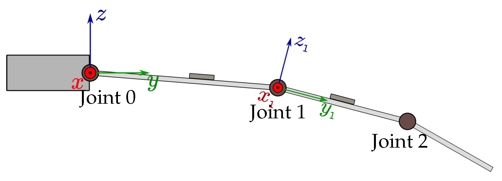
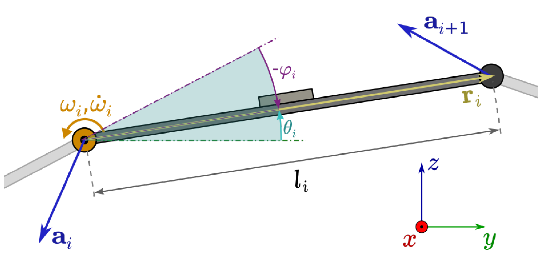
2.1. Finger Model

Finger motion limitations can be described by a kinematic model based on anatomical data from the structure of the hand. All fingers except the thumb are divided into three phalanges, in order of distance from the base: proximal, middle, and distal, connected to each other with joints.
The interphalangeal joints each have one degree of freedom, and in simple cases, all finger movements are assumed to only include flexion and extension, and thus lie in the flexion plane, as shown in Figure 5. As such, the finger can be modeled using a simplified kinematic model in the form of a flat three-link chain, corresponding to the three phalanges. Sources [23,24,25,26,27,28,29] validated this model as a fine first approximation.
Let us consider our model as a system of three rigid links (which we will also refer to as phalanges), interconnected by uniaxial hinges. Their rotation axes coincide and they are orthogonal to the axes of the phalanges. In addition, one of the phalanges, with its free end, is attached through a similar hinge to the metacarpus. The position and orientation of the metacarpus are considered to be constantly known from optical tracking. As discussed above, the phalanges are always located in the same flection plane.
This model used several orthonormal coordinate systems: the base system tied to the metacarpus and local systems linked to each of the phalanges and sensors (Figure 6). Their basic triple coordinates are denoted as e c = { x , y , z } for the metacarpus system and e k = { x k , y k , z k } for the local systems. Here, k is the phalange number, calculated from the attachment to the metacarpus. The beginning of the coordinate system of the k th phalange is the k th joint, and the beginning of the base coordinate system is the zero metacarpus joint.
The vectors x and x i are all aligned with each other and the axes of rotation of the hinges. Vectors y i are each directed along the axis of their corresponding phalange, and vectors z, z i complement the others to form an orthogonal right-handed coordinate system in R 3 .
The initial position of all coordinate systems was considered to be such that the base triples of all local systems coincided with the global base triple. For the i th phalange, we can define the angle θ i between the vectors y and y i , where the positive direction of rotation is considered to be clockwise rotation around the x axis. The angles of rotation of the hinges are: φ i = θ i θ i 1 (here θ 1 is 0).
For each phalange, we define a vector r i = l i y i , where l i is the length of the phalange.
We placed sensors on Phalanges 1 and 2. We assumed that the instrumental coordinate systems coincided with those of their corresponding phalanges, e i k , where sensor number k was placed on the i k th phalange, at a distance of p k from its proximal end. The position of the sensor relative to the proximal end of its phalange can be described by the radius vector h k = p k y i k = α k r i k (where α k = p k l i k ).
The relative position of the ends of each phalange can be in turn described by the vector r i = l i { 0 , cos θ i , sin θ i } = R i { 0 , l i , 0 } , where:
R i = R ( θ i ) = ( 1 0 0 0 cos ( θ i ) sin ( θ i ) 0 sin ( θ i ) cos ( θ i ) ) ,
is the rotation matrix corresponding to a rotation by the angle of θ i around the x axis.
Through the summation of these radius vectors, the finger’s configuration was entirely determined by either of the triples of angles: θ 0 2 or φ 0 2 . The problem of estimating the configuration of the finger was thus equivalent to the problem of estimating the set of angles φ 0 , φ 1 , φ 2 .
Let us consider the finger in motion, with the angles θ i ( t ) , angular speeds ω i ( t ) = θ ˙ i ( t ) , and angular accelerations ω ˙ i ( t ) known for all joints, as well as the acceleration of the zero joint relative to the global inertial coordinate system (Figure 7).
Denote s k as the radius vector of the k th sensor in the base coordinate system of the model, then:
s k = i = 0 i k r i + h k .
The acceleration of the sensor in an inertial coordinate system is represented as:
g k = a 0 + i = 0 i k ( [ ω i ˙ × r i ] ω i 2 r i ) + [ ω ˙ i k × h k ] ω i k 2 h k .
Here, ω ˙ = ω ˙ x i is a vector representation of the angular acceleration.
To calculate the modeled sensor’s readings, we needed to subtract the value just found from the acceleration due to gravity g and also calculate the representation of the resulting vector in the instrumental coordinate system of the sensor. Hereon, we assumed that the sensors’ coordinate systems coincided with the local coordinate axes and that their sensitivity scale factor was calibrated. With this, the readings of the k th sensor equate to:
f k = e k , g g k .

2.2. Simple Switching Tracking Algorithm

Tracking the human hand movements has important specifics with regards to the object being tracked. The wide range of possible hand movements significantly complicates the task. Goal-directed hand movements are similar in structure to eye movements [30]. Therefore, hand movement tracking can apply the oculography motion detection approach [31]. In the following paragraphs, we will formulate a criterion for switching between several types of tracking, similar to how it is done in eye tracking tasks.
Let us assume that the exact location and orientation of the metacarpus at each moment in time are known from the optical tracking data. For most simple grasping movements, we can take as the first approximation that the angle in the distal joint always equals the angle in the proximal joint [32].

2.2.1. Algorithm of The Position Estimation of The Single Phalange

Let us divide all finger motions into two distinct classes of “slow” and “fast” motion, which we define as follows:
Slow motion is the movement of the finger during which the acceleration of all of its elements relative to the wrist is negligible compared to the acceleration due to gravity. All other movement is classified as fast motion.
Fast motions are characterized by large angular velocities, phalange accelerations, and a rather short duration because of the fact that the extent of finger movement is limited. Slow motions, on the other hand, have a significantly longer total duration than fast ones and are are typically represented by maintaining a fixed finger configuration.
This leads to the idea of using two different estimation algorithms for different motion classes and switching between them when moving from one class to another.

2.2.2. Slow Motion Estimation

We can consider a slow motion using the kinematic model described above.
Let us define the local acceleration of a sensor as:
μ k = s ¨ k .
From Equations (4) and (3), we get:
g k = a 0 + μ k ; | μ k | ( i k + 1 ) | g | .
Since we know the movement of the wrist, we also know the representation f = { f 1 , f 2 , f 3 } of the vector g c = a 0 g in the base coordinate system of the model e c .
By definition, f j = e c j , g c , and g c = j = 1 3 f j e k .
We similarly define the representation f of the acceleration of a sensor in the basis e = { e 1 , e 2 , e 3 } of the instrumental coordinate system of the sensor: f j = e j , g c
We can state that:
i = 1 3 f i e k = g = g c + μ = i = 1 3 f i e k + μ ; | μ | | g | .
As such, θ i can be estimated via the function atan 2 ( f 3 , f 2 ) , defined as follows:
atan 2 ( y , x ) = arctan ( y x ) , x > 0 ; arctan ( y x ) + π sign y , x < 0 ; π 2 sign y , x = 0 .

2.2.3. Fast Movement Estimation

Let us consider now a fast motion. According to our definition, it is a transition between periods of slow motion, where the time of this movement is much less than one second. If we assume that at the beginning of the motion, the finger configuration is known to the system with acceptable accuracy, then we can calculate the orientation of the phalange by integrating the measured angular velocities based on the known initial position:
θ i , t = int ( θ i , t 1 , ω ) ,
where int ( i ) is a function performing a step of a numerical integration algorithm.
The accumulated error due to integration can later be corrected during the following phase of slow motion.

2.2.4. Errors in The Estimation Algorithms for Slow and Fast Motion

Let us define the errors:
Δ θ ω error of the fast movement estimation algorithm ( AVS integration ) , Δ θ g error of the slow movement estimation algorithm ( from measured acceleration g ) , Δ θ estimation the deviation of the composite estimation algorithm .
We will now estimate the deviation magnitude of the slow movement estimation algorithm. Suppose that angular velocities do not exceed ω max , angular accelerations do not exceed ω ˙ max , and phalanges are no longer than l max . Therefore, the magnitude of the accelerations is limited by:
| r ¨ i | l max ω ˙ max 2 + ω max 4 .
Thus, the value μ from (5) corresponds to:
| μ | < ( i k + 1 ) l max ω ˙ max 2 + ω max 4 .
Now, consider how the deviation of orientation estimation Δ θ g depends on g and μ . Since a flat model is used, the algorithm only considers the components of accelerations within the flexion plane y z . Taking into account that for small angles tan ( x ) x and that the maximum estimation error is attained when μ g , we can estimate the error magnitude for phalange k using (6):
| θ g | k | μ | | g y z | < ( i k + 1 ) l max ω ˙ max 2 + ω max 4 | g y z | .
From (7), it follows that for identical finger movements, the accuracy of the estimate from observing the vector g diminishes as the magnitude of the in-plane component of g decreases. Ultimately, if the flexion plane is horizontal, the estimation error can become arbitrarily large, and the estimate carries no actual information. In this case, the only available way to determine orientation is through integration of AVS readings.
The integration error, on the other hand, grows linearly with time: | Δ θ ω ( t ) | | Δ ω | t , where | Δ ω | characterizes the average AVS deviation.

2.2.5. Switching Algorithm

For the proposed algorithm to perform optimally, the switching criterion has to minimize the general deviation of the overall estimate of the phalange’s orientation.
Consider some possible arbitrary movements. The deviation of the slow motion estimation algorithm is then a time dependent function:
Δ θ g = Δ θ g ( t ) .
In turn, the total error during fast motion estimation has the form:
Δ θ ω = Δ θ ω ( t t s ) + Δ θ g ( t s ) ,
where t s is the time of the last switch to integration. In the worst case, error accumulation is going in the same direction as the previous deviation of the slow motion algorithm, giving us an upper bound:
| Δ θ ω ( t , t s ) | = | Δ ω | · ( t t s ) + | Δ θ g ( t s ) | .
We divide time into discrete intervals t 1 t n and introduce an estimate of the error at the ith time moment:
Δ θ ˜ ( t i ) = Δ θ ˜ g ( t i ) , if the slow motion estimation algorithm is currently used ; Δ θ ˜ ω ( t i , t s ) , if the fast motion estimation algorithm is currently used .
The estimates Δ θ ˜ g ( t ) and Δ θ ˜ ω ( t ) are defined according to (7) and (8). For each time interval, we choose the algorithm that minimizes the estimate of the total error Δ θ ˜ . From (8), it follows that for each moment, an integration step would yield an error of no more than Δ θ ( t k + 1 ) | ω = Δ θ ( t k ) + ( t k + 1 t k ) · | Δ ω | , independent of t s . This value can be directly compared with Δ θ g ( t i ) .
Thus, the final estimation algorithm is as follows:
1.
receive sensor readings a ^ , ω ^ ;
2.
calculate Δ θ g ( t i ) = | μ ˜ | ( ω ^ ) | g x y | and Δ θ ( t i ) | ω = Δ θ ( t i 1 ) + ( t i t i 1 ) · | Δ ω | ;
3.
choose the estimation mode:
  • if currently in fast motion mode and Δ θ g ( t i ) < Δ θ ( t i ) | ω , then switch to slow motion mode, and assign Δ θ ( t i ) : = Δ θ g ( t i ) ;
  • if currently in slow motion mode and Δ θ ( t i ) | ω < Δ θ g ( t i ) , then switch to fast motion mode, taking θ ˜ ( t i 1 ) as the initial estimate, and assign Δ θ ( t i ) : = Δ θ ( t i ) | ω .
4.
Calculate a new orientation estimate θ ˜ using the currently selected estimation algorithm.

2.3. Madgwick Filter Modification

The Madgwick filter algorithm suggested in [20] is used for the restoration of body orientation according to the readings of microelectromechanical sensors. Usually, the filter is presented in two modifications. The first modification can be used for INS (Inertial Navigation Systems), which consist of only a three-axis accelerometer and AVS. The second is applied to INS that also contain a three-axis magnetometer. A three-axis magnetometer measures the Earth’s magnetic field vector together with local magnetic distortions. This complicates its use in rooms with VR equipment, metal structures, and other objects that cause large distortions in the magnetic field.
We propose a modified Madgwick filter, taking into account the features of the kinematic model of a finger. Instead of the magnetic field induction vector, we can take the normal axis of the flexion plane as the second correction vector. This modification will always work correctly except in the case of the co-directionality of the correction vectors, which, due to its rarity, we can neglect.

2.3.1. Finger Rotation Estimation

Let us describe our proposed modified Madgwick filter. Hereafter, we will use the quaternion apparatus to represent rotations.
In this section, the sign ⊗ shall denote the operation of quaternion multiplication. A tilde over a variable · ˜ denotes the estimate of the corresponding quantity, and a circumflex · ^ denotes its measured value. The subscript before a variable indicates the target coordinate system. A superscript indicates the coordinate system with respect to which the variable is specified. E and S k denote, respectively, the global coordinate system tied to the Earth and the instrumental coordinate system of sensor k.
In particular, we introduce the quaternion S k E q ˜ to describe the estimate of the sensor’s orientation relative to the Earth, and the vectors S k f ^ to denote acceleration and angular velocity measurements in the sensor’s coordinate system.
From:
E S k q ˙ = 1 2 E S k q S k ω .
and having the readings of the sensors and the previous orientation estimate E S k q ˜ t 1 (which is initially taken from the optical tracking data), we can get an estimate E S k q ˜ ω , t of the sensor’s orientation relative to the ground:
E S k q ˜ ω , t = E S k q ˜ t 1 + Δ t 2 ( E S k q ˜ t 1 S k ω ^ ) .
When constructing the orientation filter, it is assumed that the accelerometer will measure only acceleration due to gravity, and we know the plane of motion from the readings of the optical system on the metacarpus.
Let us calculate another estimate by solving a problem of numerical optimization for the desired quaternion, in which as the initial approximation, we take a previous estimate E S k q ˜ t 1 , and as the cost function, we take the measure of the accuracy of vector alignment achieved by the desired rotation:
| | J ( E S k q ˜ , E g , E g k S k g ^ ) | | min E S k q ˜ R 4 J ( E S k q ˜ , E g , S k f ^ ) = E S k q ˜ ( E g E g k ) E S k q ˜ 1 S k f ^ ;
where J is the cost function, S k f ^ are the accelerometer measurements in the coordinate system of the sensor, E g is a known gravity vector in the global coordinate system, and E g k is a vector obtained from (2) using current sensor data and past orientation estimates E S k q ˜ t 1 in the global coordinate system.
The problem is solved by the gradient descent method. The only possible solution is chosen, taking into account the normal to the flexion plane, known from the optical tracking data. The estimate E S k q ˜ , t of the sensor orientation relative to the ground is obtained:
E S k q ˜ , t = E S k q ˜ t 1 μ t J | | J | | .
The optimal value μ t depends on the rotation speed and can be calculated based on the readings of the angular velocity sensors [20]:
μ t = α | | E S k q ˙ ω , t | | Δ t ; α > 1 .

2.3.2. Combining Filter Algorithm

Obtaining estimates E S k q ˜ ω , t from the angular velocity and E S k q ˜ , t from the observations of known vectors, we can determine the joint estimate as a linear combination with weights γ t , ( 1 γ t ) , similar to the classic Madgwick filter:
E S k q ˜ + , t = γ t E S k q ˜ , t + ( 1 γ t ) E S k q ˜ ω , t , 0 < γ t < 1 .
Given that both estimates E S k q ˜ ω , t and E S k q ˜ , t are obtained from the previous general estimate E S k q ˜ t 1 by adding small terms to it E S k q ˙ ω , t Δ t and α | | E S k q ˙ ω , t | | Δ t J | | J | | , we get:
E S k q ˜ + , t = E S k q ˜ t 1 + E S k q t ˜ ˙ Δ t ,
E S k q t ˜ ˙ = ( 1 γ t ) E S k q ˙ ω , t + γ t E S k q ˙ ϵ , t ,
E S k q ˙ ϵ , t = 1 Δ t μ t J | | J | | .
According to the article [20], the parameter γ t can be considered small, and by replacing γ t = β Δ t μ t , where β is a small number, we can simplify the expression (16):
E S k q t ˜ ˙ = E S k q ˙ ω , t β J | | J | | .
Additionally, since the described operations do not guarantee the preservation of the unit norm of the quaternion, the resulting estimate must be normalized:
E S k q ˜ t = E S k q ˜ + , t | | E S k q ˜ + , t | | .
The expressions (15), (18), and (19) define the final form of the filter.
It is possible to use a non-constant value for parameter β , changing it depending on the current motion, decreasing by large values with spurious accelerations μ . This can further improve filter accuracy by reducing the impact of accelerometer errors on estimation during fast movements.

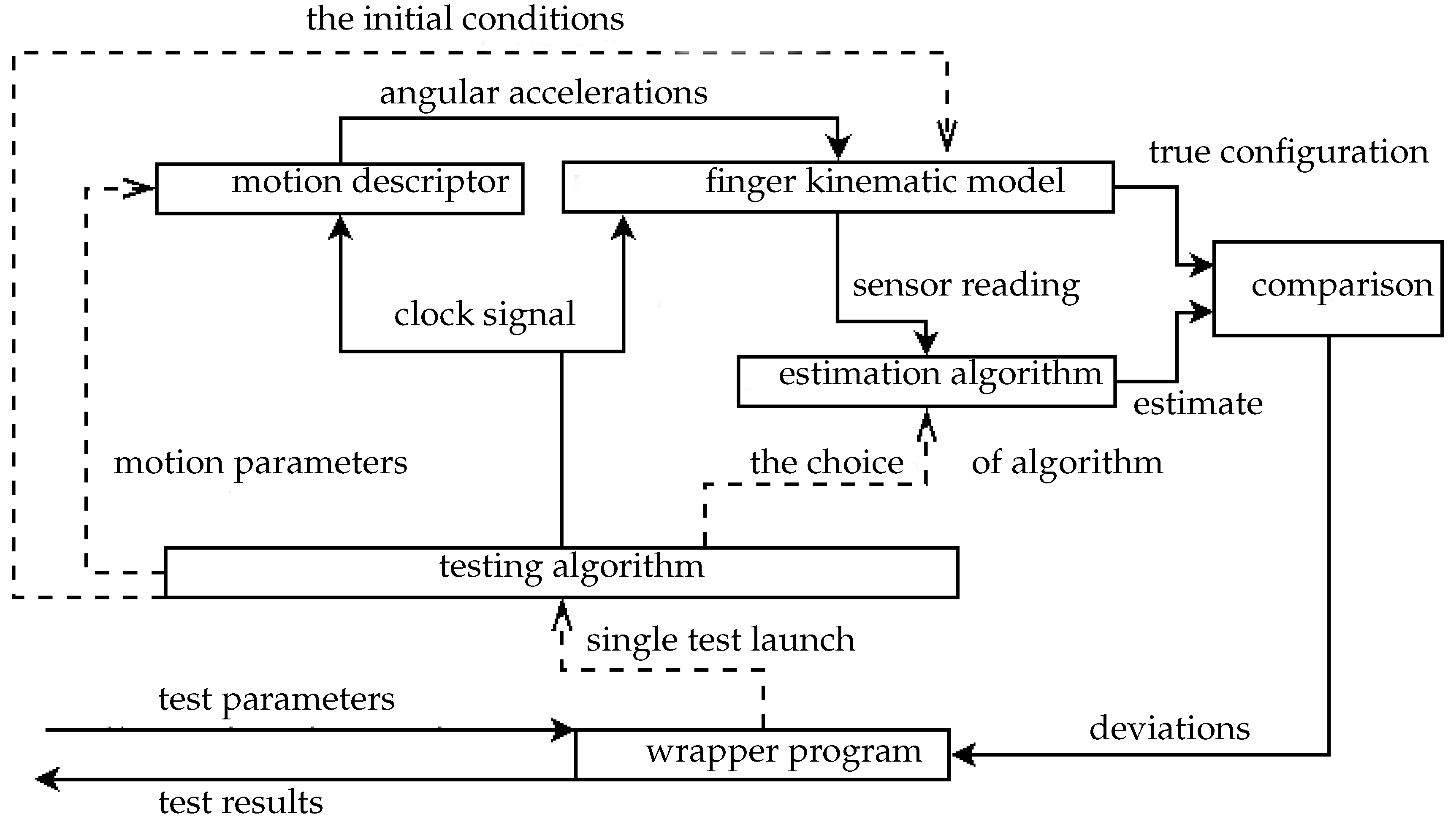
3. Verification of Algorithms Using Numerical Model Data

A mathematical simulation system was developed using Python in order to generate virtual sensor outputs and to use them to verify the correct operation of both estimation algorithms experimentally.
The simulation system was logically divided into several blocks:
  • a model of a moving finger equipped with inertial sensors,
  • a set of parametric descriptors for some groups of finger movements,
  • implementations of the simple switching algorithm and the modified Madgwick filter,
  • a wrapper program applying logic to conducting tests of estimation algorithms on generated model data.
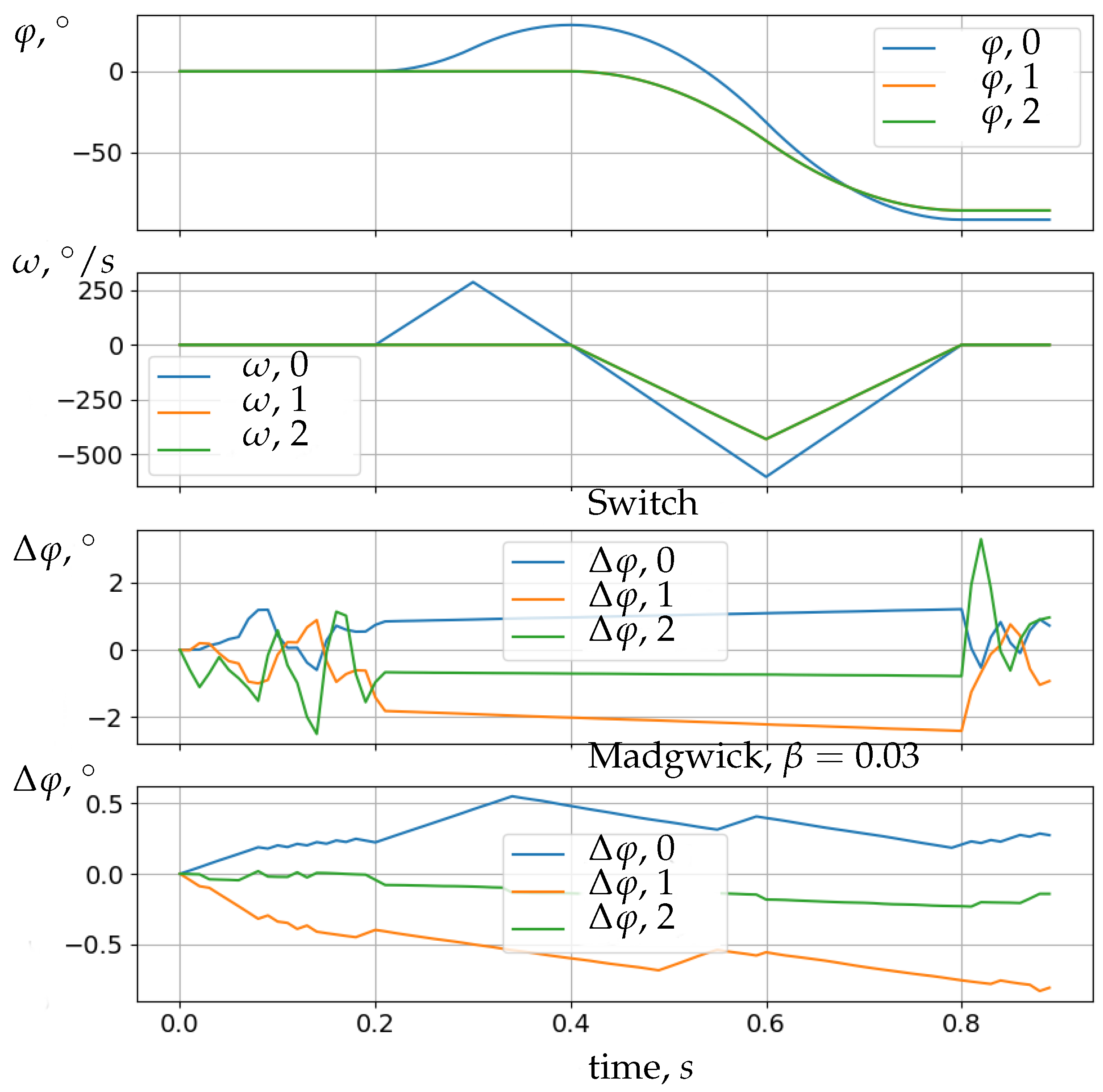
A diagram of the testing system and the interaction of its elements during operation is presented in Figure 8.
For the numerical integration in the fast motion estimator, the Runge–Kutta method [33] was used, the numerical error of which can be considered negligible compared to the accumulation of errors due to noise and sensory errors. The modified Madgwick filter was implemented in the first (flat model) variant and with a static β parameter.
The algorithms were tested on identical motions in order to compare their accuracy depending on the parameters of the test movement. For comparative tests, a parametric class of complex motions imitating grasping was used. The test motion had the following structure:
  • A static interval lasting t d ;
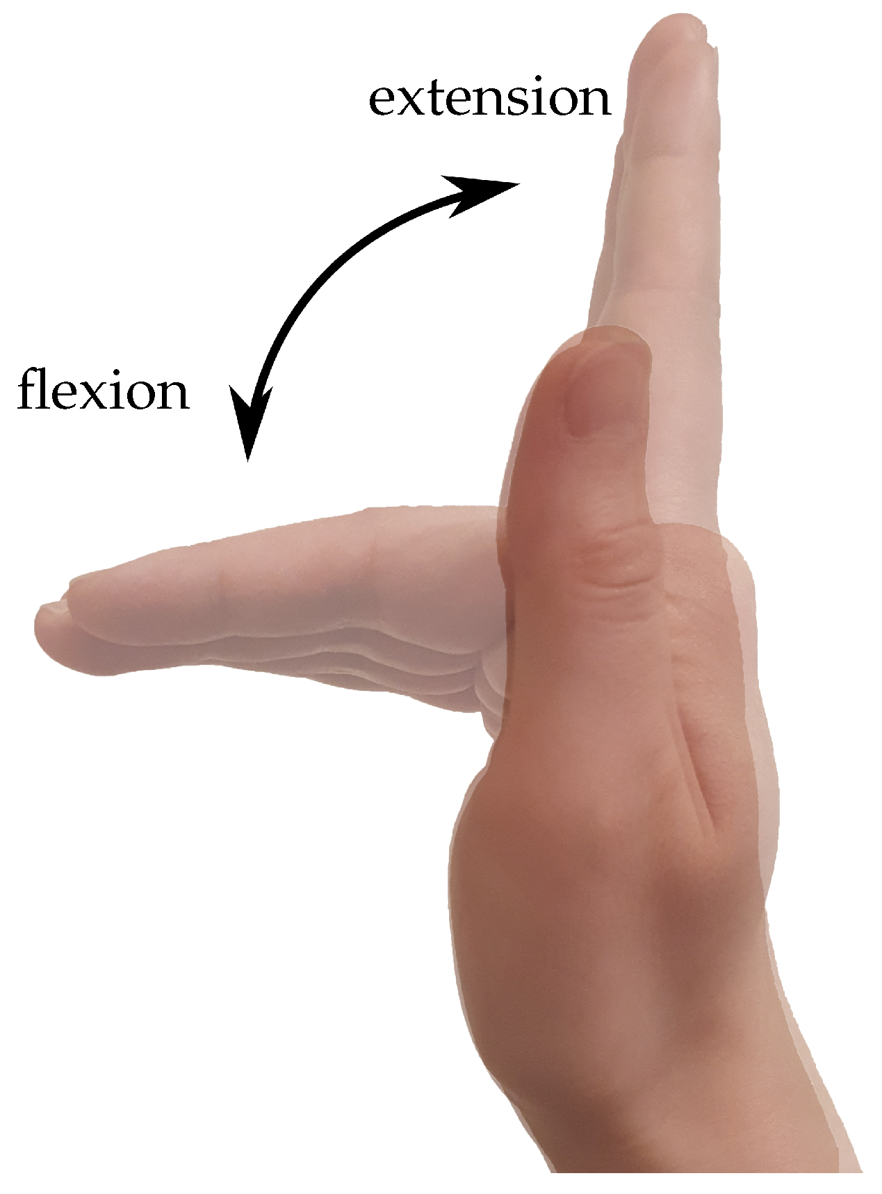
  • The extension of a straight finger in the MCPjoint (Joint 0) to a 28 angle lasting 1 3 t m ;
  • Simultaneous flexion of the finger in Joint 0 to 90 and in the interphalangeal (1 and 2) joints to an angle of 85 lasting 2 3 t m .
The tests were carried out in the following order:
  • Initial conditions for the kinematic model of the finger were specified. This position was considered as the known accurate initial estimate.
  • The motion and its parameters were specified.
  • The modeling of a given movement was performed, during which we collected data with a given sampling rate:
    -
    the readings of virtual sensors were calculated and transferred to the evaluation algorithm with the addition of sensor errors;
    -
    the current true configuration (phase coordinates and speeds) of the finger model and the configuration estimate by the algorithm were recorded.
  • After the simulation was completed, a measure of the deviation of the estimate from the actual configuration was calculated.
Three series of tests were carried out, differing in the errors added to the readings of the virtual sensors:
  • with white noise;
  • with a zero offset;
  • with errors of both kinds.
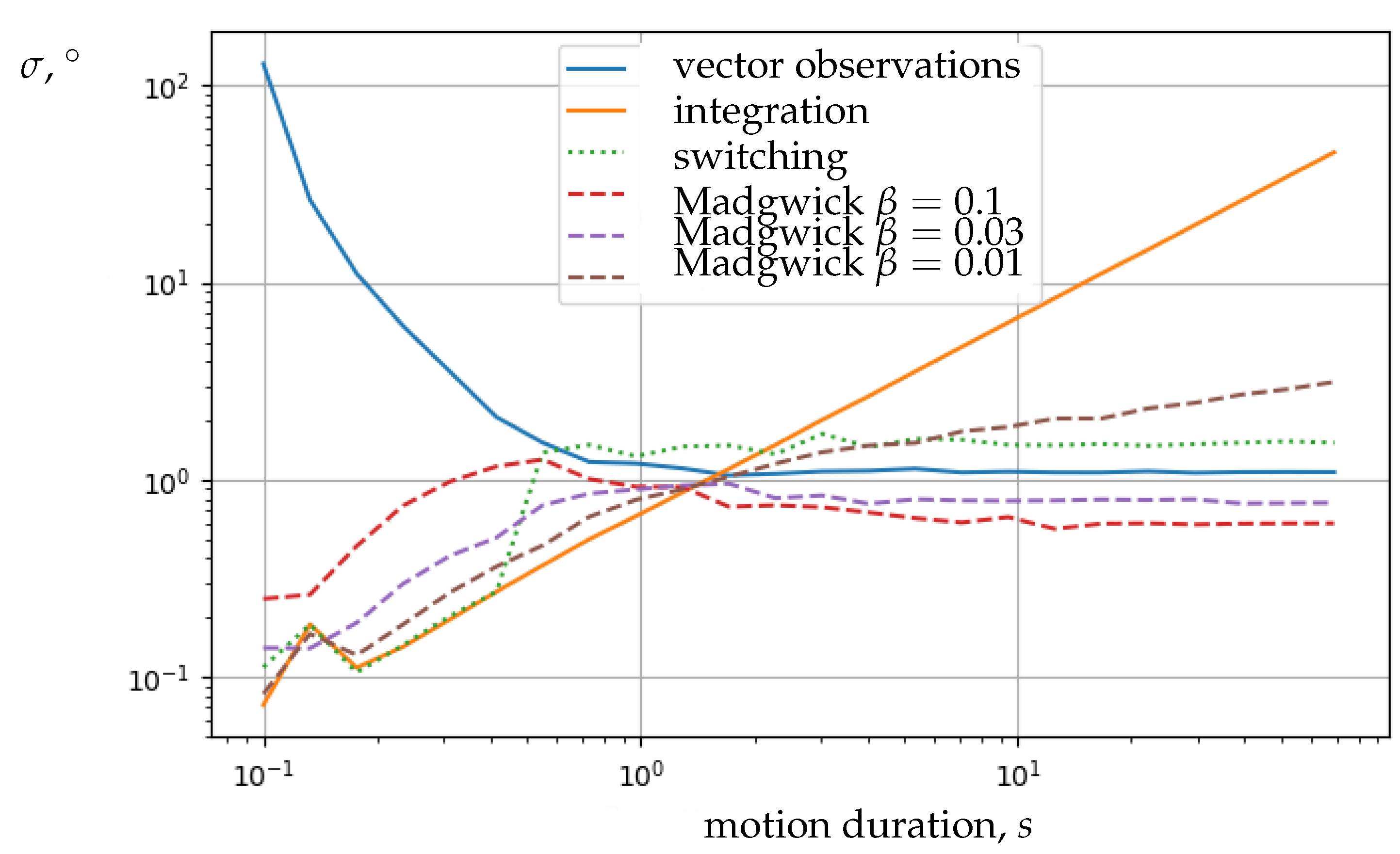
The values of the simulated errors corresponded to the characteristics of the MPU-9250 [34] microelectromechanical inertial sensor.
In each series, there were 32 movements, differing from each other by the parameter of the time of movement t m , which varied from 0.1 to 10 3 s, with the same delay t d = 0.2 s at the start of the movement. Each movement of the series was used to simulate the readings of the sensors to calculate the input sent to the estimation algorithms and to calculate the estimation error of the algorithm during the motion.

Test Results

Figure 9 demonstrates the example of the the characteristic deviations of the estimate given by the proposed algorithms. The top two charts show the true trajectory of the finger, while the bottom two show the deviation of the estimate.
The Madgwick filter was significantly better at dampening the high-frequency sensor noise compared to the simple switching algorithm, and the influence of disturbances affected the algorithm’s accuracy only after a while. This was also a drawback, however, as a similar amount of time was needed to restore accuracy after the disturbance, while the error in the switching algorithm immediately returned to near zero as soon as the fast movement stopped.
Figure 10 shows a graph of the RMS (Root-Mean-Square) of the algorithms’ estimation error over the course of the whole movement in relation to its duration.
As we can see, with the presence of systematic sensory errors, pure integration began to outperform the pure gravity vector observation algorithm for motion durations on the order of one second. The switching algorithm and the Madgwick filter showed similar accuracy, but we could also see here that noise had a much greater influence on the simple switching algorithm. At the same time, the Madgwick filter’s sensitivity to the choice of the β parameter was clearly visible: too high a value led to an increased error during fast movements, while too low a value led to the divergence of the estimate over time due to insufficient compensation for the accumulation of the integration error.
Both algorithms demonstrated satisfactory accuracy, only limited by the errors of the accelerometer. In terms of calculation speed, the switching algorithm proved itself to be only slightly (about 10%) faster than the Madgwick filter.

4. Discussion

In this article we considered a pair of algorithms for tracking one phalange in the flexion plane for different modes of movement. Their accuracy was analyzed and a criterion for the separation of modes has been identified. A hybrid algorithm was constructed to combine these algorithms by switching between different positioning modes. We proposed an extension of the Madgwick filter in order to track the configuration of a moving finger, taking into account its structure and available information about the position and orientation of the metacarpus.
The described algorithms were implemented and tested on data obtained using a software model of flat finger movement. We also carried out an analysis of the nature of the algorithms’ errors and the accuracy of the estimates obtained by them, depending on the speed of movement. Both solutions demonstrated an appropriate quality for the defined task.
The proposed algorithms allowed us to circumvent the limitations of inertial sensors described in the Introduction. Unlike [14,15,18,35], our method did not require magnetometers and, as a result, was not sensitive to changes in the magnetic field. Compared to [16,22], we used fewer inertial sensors, which thus simplified the design of the inertial glove. The magnitude of our algorithm’s errors on simulated movements was comparable to those from the works cited above. Finally, our method did not require additional calibration and a resetting procedure before each launch.
The advantages of the hybrid tracking approach led us to the in-out tracking systems for VR: we could combine markerless head tracking with inertial body and hand configuration tracking. Compared to classic out-in VR systems, this solution was not bound by the space of the hosting room. In most cases, our reconstructed objects consisted of many elements with sizes ranging from 50 cm to 15 m, but some important architectural details were even smaller. Hand interaction with small details felt more familiar to many researchers. The markerless aspect of the proposed solution made it very practical for augmented reality applications.
The obtained results are to be used in the VR systems for the virtual historical reconstruction of Moscow’s city center. We are aiming to develop a convenient and user-friendly interaction system with VR for displaying data similar to those described in [36].

Author Contributions

Methodology, L.B., S.L., M.M., and V.C.; software, I.U. and M.B.; validation, L.B. and S.L.; investigation, I.U.; formal analysis, A.K. and V.C.; writing, original draft preparation, I.U., V.C., A.K., M.M., and M.B.; writing, review and editing, V.C., L.B., M.M., M.B., and A.K.; visualization, M.M.; project administration, S.L.; supervision, L.B. All authors read and agreed to the published version of the manuscript.

Funding

The research is supported by the Russian Foundation for Basic Research Grant 18-00-01684 (K) (18-00-01590 and 18-00-01641).

Conflicts of Interest

The authors declare no conflict of interest.

Abbreviations

The following abbreviations are used in this manuscript:
IMUInertial Measurement Unit
AVSAngular Velocity Sensor
INSInertial Navigation System
RMSRoot-Mean-Square
VRVirtual Reality

References

  1. Lemak, S.; Chertopolokhov, V.; Kruchinina, A.; Belousova, M.; Borodkin, L.; Mironenko, M. O zadache optimizatsii raspolozheniya elementov interfeysa v virtual’noy real’nosti (v kontekste sozdaniya virtual’noy rekonstruktsii istoricheskogo rel’yefa Belogo goroda). Istor. Inform. 2020, 67–76. [Google Scholar] [CrossRef] [Green Version]
  2. Borodkin, L.; Mironenko, M.; Chertopolokhov, V.; Belousova, M.; Khlopikov, V. Tekhnologii virtual’noy i dopolnennoy real’nosti (vr/ar) v zadachakh rekonstruktsii istoricheskoy gorodskoy zastroyki (na primere moskovskogo Strastnogo monastyrya). Istor. Inform. 2018, 76–88. [Google Scholar] [CrossRef]
  3. Figueiredo, L.; Rodrigues, E.; Teixeira, J.; Teichrieb, V. A comparative evaluation of direct hand and wand interactions on consumer devices. Comput. Graph. 2018, 77, 108–121. [Google Scholar] [CrossRef]
  4. Wachs, J.; Stern, H.; Edan, Y.; Gillam, M.; Feied, C.; Smith, M.; Handler, J. A Real-Time Hand Gesture Interface for Medical Visualization Applications. In Applications of Soft Computing; Tiwari, A., Roy, R., Knowles, J., Avineri, E., Dahal, K., Eds.; Springer: Berlin/Heidelberg, Germany, 2006; pp. 153–162. [Google Scholar]
  5. Tamura, H.; Liu, J.; Luo, Y.; Ju, Z. An Interactive Astronaut-Robot System with Gesture Control. Comput. Intell. Neurosci. 2016. [Google Scholar] [CrossRef] [Green Version]
  6. Yang, L.; Jin, H.; Feng, T.; Hong-An, W.; Guo-Zhong, D. Gesture interaction in virtual reality. Virtual Real. Intell. Hardw. 2019, 1, 84–112. [Google Scholar] [CrossRef]
  7. Bugrov, D.; Lebedev, A.; Chertopolokhov, V. Estimation of the angular rotation velocity of a body using a tracking system. Mosc. Univ. Mech. Bull. 2014, 69, 25–27. [Google Scholar] [CrossRef]
  8. Colyer, S.; Evans, M.; Cosker, D.; Salo, A. A Review of the Evolution of Vision-Based Motion Analysis and the Integration of Advanced Computer Vision Methods Towards Developing a Markerless System. Sports Med. Open 2018, 4, 24. [Google Scholar] [CrossRef] [PubMed] [Green Version]
  9. Wang, L.; Meydan, T.; Williams, P. A Two-Axis Goniometric Sensor for Tracking Finger Motion. Sensors 2017, 17, 770. [Google Scholar] [CrossRef] [Green Version]
  10. Zhang, Z. The Design and Analysis of Electromagnetic Tracking System. J. Electromagn. Anal. Appl. 2013, 5, 85–89. [Google Scholar] [CrossRef] [Green Version]
  11. Paperno, E.; Sasada, I.; Leonovich, E. A new method for magnetic position and orientation tracking. Magn. IEEE Trans. 2001, 37, 1938–1940. [Google Scholar] [CrossRef]
  12. Raab, F.; Blood, E.; Steiner, T.; Jones, H.R. Magnetic position and orientation tracking system. IEEE Trans. Aerosp. Electron. Syst. 1979, 15, 709–718. [Google Scholar] [CrossRef]
  13. Vavilova, N.B.; Golovan, A.A.; Parusnikov, N.A. Problem of information equivalent functional schemes in aided inertial navigation systems. Mech. Solids 2008, 43, 391–399. [Google Scholar] [CrossRef]
  14. Choi, Y.; Yoo, K.; Kang, S.; Seo, B.; Kim, S.K. Development of a low-cost wearable sensing glove with multiple inertial sensors and a light and fast orientation estimation algorithm. J. Supercomput. 2016, 74. [Google Scholar] [CrossRef]
  15. Lin, B.S.; Lee, I.J.; Yang, S.Y.; Lo, Y.C.; Lee, J.; Chen, J.L. Design of an Inertial-Sensor-Based Data Glove for Hand Function Evaluation. Sensors 2018, 18, 1545. [Google Scholar] [CrossRef] [Green Version]
  16. Salchow-Hömmen, C.; Callies, L.; Laidig, D.; Valtin, M.; Schauer, T.; Seel, T. A Tangible Solution for Hand Motion Tracking in Clinical Applications. Sensors 2019, 19, 208. [Google Scholar] [CrossRef] [Green Version]
  17. Bellitti, P.; Bona, M.; Borghetti, M.; Sardini, E.; Serpelloni, M. Sensor Analysis for a Modular Wearable Finger 3D Motion Tracking System. Proceedings 2018, 2, 1051. [Google Scholar] [CrossRef] [Green Version]
  18. Bellitti, P.; Angelis, A.; Dionigi, M.; Sardini, E.; Serpelloni, M.; Moschitta, A.; Carbone, P. A Wearable and Wirelessly Powered System for Multiple Finger Tracking. IEEE Trans. Instrum. Meas. 2020, 69, 2542–2551. [Google Scholar] [CrossRef]
  19. Maereg, A.; Secco, E.; Agidew, T.; Reid, D.; Nagar, A. A Low-Cost, Wearable Opto-Inertial 6-DOF Hand Pose Tracking System for VR. Technologies 2017, 5, 49. [Google Scholar] [CrossRef] [Green Version]
  20. Madgwick, S.; Harrison, A.; Vaidyanathan, R. Estimation of IMU and MARG orientation using a gradient descent algorithm. In Proceedings of the International Conference on Rehabilitation Robotics, Zurich, Switzerland, 29 June–1 July 2011; p. 5975346. [Google Scholar] [CrossRef]
  21. Lin, B.S.; Lee, I.J.; Chiang, P.Y.; Huang, S.Y.; Peng, C.W. A Modular Data Glove System for Finger and Hand Motion Capture Based on Inertial Sensors. J. Med. Biol. Eng. 2019, 39, 532–540. [Google Scholar] [CrossRef] [Green Version]
  22. Laidig, D.; Lehmann, D.; Bégin, M.A.; Seel, T. Magnetometer-free Realtime Inertial Motion Tracking by Exploitation of Kinematic Constraints in 2-DoF Joints. In Proceedings of the 41st Annual International Conference of the IEEE Engineering in Medicine and Biology Society (EMBC), Berlin, Germany, 23–27 July 2019; Volume 2019, pp. 1233–1238. [Google Scholar] [CrossRef]
  23. Hulst, F.; Schätzle, S.; Preusche, C.; Schiele, A. A functional anatomy based kinematic human hand model with simple size adaptation. In Proceedings of the IEEE International Conference on Robotics and Automation, St Paul, MN, USA, 14–19 May 2012; pp. 5123–5129. [Google Scholar] [CrossRef] [Green Version]
  24. Buchholz, B.; Armstrong, T. A kinematic model of the human hand to evaluate its prehensile capabilities. J. Biomech. 1992, 25, 149–162. [Google Scholar] [CrossRef] [Green Version]
  25. Cobos, S.; Ferre, M.; Uran, M.; Ortego, J.; Peña Cortés, C. Efficient Human Hand Kinematics for Manipulation Tasks. In Proceedings of the IEEE/RSJ International Conference on Intelligent Robots and Systems, Nice, France, 22–26 September 2008; pp. 2246–2251. [Google Scholar] [CrossRef] [Green Version]
  26. Chen, F.; Appendino, S.; Battezzato, A.; Favetto, A.; Mousavi, M.; Pescarmona, F. Constraint Study for a Hand Exoskeleton: Human Hand Kinematics and Dynamics. J. Robot. 2013, 2013. [Google Scholar] [CrossRef] [Green Version]
  27. Chao, E.Y.S.; An, K.N.; Cooney, W.P.; Linscheid, R.L. Normative Model of Human Hand; World Scientific: Singapore, 1989. [Google Scholar]
  28. Lenarčič, J.; Bajd, T.; Stanišić, M. Kinematic Model of the Human Hand. In Robot Mechanisms; Springer: Berlin, Germany, 2013; pp. 313–326. [Google Scholar]
  29. Stillfried, G. Kinematic Modelling of the Human Hand for Robotics. Ph.D. Thesis, Technische Universitat Munchen, Munchen, Germany, 2015. [Google Scholar]
  30. van Beers, R.; Sittig, A.; van der Gon, J. Integration of proprioceptive and visual position-information: An experimentally supported model. J. Neurophysiol. 1999, 81, 1355–1364. [Google Scholar] [CrossRef] [PubMed]
  31. Bokov, T.; Suchalkina, A.; Yakusheva, E.; Yakushev, A. Mathematical modelling of vestibular nystagmus. Part I. The statistical model. Russian J. Biomech. 2014, 18, 40–56. [Google Scholar]
  32. DEXMART. Kinematic Modelling of the Human Hand; Technical Report; Dexmart Deliverable D1.1: Napoli, Italy, 2009. [Google Scholar]
  33. Hazewinkel, M. Encyclopedia of Mathematics; Springer Science+Business Media B.V.; Kluwer Academic Publishers: Berlin, Germany, 1994. [Google Scholar]
  34. InvenSense, I. MPU-9250 Product Specification; Revision 1.1; InvenSense Inc.: San Hosem CA, USA, 2014. [Google Scholar]
  35. Fahn, C.S.; Sun, H. Development of a Fingertip Glove Equipped with Magnetic Tracking Sensors. Sensors 2010, 10, 1119–1140. [Google Scholar] [CrossRef]
  36. Borodkin, L.I.; Valetov, T.Y.; ZHerebyat’ev, D.I.; Mironenko, M.S.; Moor, V.V. Reprezentaciya i vizualizaciya v onlajne rezul’tatov virtual’noj rekonstrukcii. Istor. Inform. 2015, 3–4, 3–18. [Google Scholar]
Figure 1. Example of a projected image.
Computers 09 00040 g001
Figure 2. Example of the VR interactive verification module.
Computers 09 00040 g002
Figure 3. Map level of the verification module.
Computers 09 00040 g003
Figure 4. Hand tracking device combined with vibro-tactile output.
Computers 09 00040 g004
Figure 5. Flexion and extension of the human hand.
Computers 09 00040 g005
Figure 6. General structure of the kinematic model of a finger and the coordinate systems used.
Computers 09 00040 g006
Figure 7. Angles and vectors used in the model.
Computers 09 00040 g007
Figure 8. Structure of the testing software.
Computers 09 00040 g008
Figure 9. Motion and comparison of the algorithm’s errors.
Computers 09 00040 g009
Figure 10. The RMS error of different estimation algorithms with relation to test motion duration.
Computers 09 00040 g010

