To Adapt or Not to Adapt: A Quantification Technique for Measuring an Expected Degree of Self-Adaptation ^†

Abstract

Self-adaptation and self-organization (SASO) have been introduced to the management of technical systems as an attempt to improve robustness and administrability. In particular, both mechanisms adapt the system’s structure and behavior in response to dynamics of the environment and internal or external disturbances. By now, adaptivity has been considered to be fully desirable. This position paper argues that too much adaptation conflicts with goals such as stability and user acceptance. Consequently, a kind of situation-dependent degree of adaptation is desired, which defines the amount and severity of tolerated adaptations in certain situations. As a first step into this direction, this position paper presents a quantification approach for measuring the current adaptation behavior based on generative, probabilistic models. The behavior of this method is analyzed in terms of three application scenarios: urban traffic control, the swidden farming model, and data communication protocols. Furthermore, we define a research roadmap in terms of six challenges for an overall measurement framework for SASO systems.

1. Introduction

Information and communication technology faces a trend towards increasingly complex solutions, e.g., characterized by the laws of Moore [1] and Glass [2]. Consequently, traditional concepts for design, development, and maintenance have reached their limits. Within the last decade, a paradigm shift in engineering such systems has been postulated that claims to master complexity issues by means of self-adaptation and self-organization. Concepts and techniques emerged that move traditional design-time decisions to runtime and from the system engineer to the systems themselves. As a result, the self-adapting and self-organizing (SASO) systems domain serves as an umbrella for heterogeneous research initiative focusing on these issues, including e.g., Organic Computing [3], Autonomic Computing [4], Interwoven Systems [5], or Self-aware Computing Systems [6].

The fundamental idea behind these concepts is to master complexity while simultaneously improving scalability and robustness through distributed decisions of smaller, more simple entities that act at a local basis and adapt their behavior according to observed environmental conditions. At the same time, these individual entities (also called agents or subsystems) cooperate to achieve a global system goal. As a result, a variety of adaptation mechanisms, self-organization algorithms, and cooperation schemes, architectures and design processes or interaction protocols have been developed, resulting in various kinds of SASO systems.

The presented development of different SASO systems often assumes that self-adaptation is always desired, since each re-configuration or change of the current behavior is done to optimize a certain system goal or utility function. Examples range from the initial vision for Autonomic Computing [4], over concepts based on control theory [7], to those from the Organic Computing domain [8]. A comprehensive study on engineering approaches for SASO systems can be found in [9]. Within this list of contributions, only a few determine a maximum number of adaptations. In turn, most of the approaches trigger adaptation as a response to detected changes without considering the number of changes done so far or the severity of the performed changes. The actual maximum number of adaptations is usually given by the frequency with which the control module is performed (i.e., in each of these cycles a decision is taken if an adaptation is triggered or not).

In scenarios where the SASO systems acts without user contact, the primary negative implication of such frequent modifications of the behavior is the decreasing stability, and possible chain reactions of adaptations of other systems to the new configurations (as, e.g., considered in the context of mutual influences, see [10]). However, as soon as a human is interacting with a technical system, too frequent modifications may decrease acceptance.

Furthermore, we argue in this position paper that a theoretical limitation is not the best approach: All adaptations come with drawbacks, e.g., decreased stability or reduced comprehensibility for users. Consequently, we argue that there must be some kind of “optimal degree of self-adaptation” in a SASO system, most certainly depending on the current conditions (e.g., the presence of disturbances). To be able to determine such an optimal self-adaptation behavior, we have to provide a measurement basis for quantifying these effects in the first place, ideally integrated into a unified overall framework for measuring and analyzing properties of SASO systems. In particular, we need to address the following basic questions:

• How can we quantify the observed adaptation effort within a large-scale SASO system consisting of a possibly large set of autonomous entities or subsystems?
• How can we derive statements about the stability of configurations if self-adaptation of the individual entities/subsystems are continuously happening and desired?
• How can we determine an expected degree of self-adaptation of this overall SASO system according to a given environmental context (or a ’situation’)?

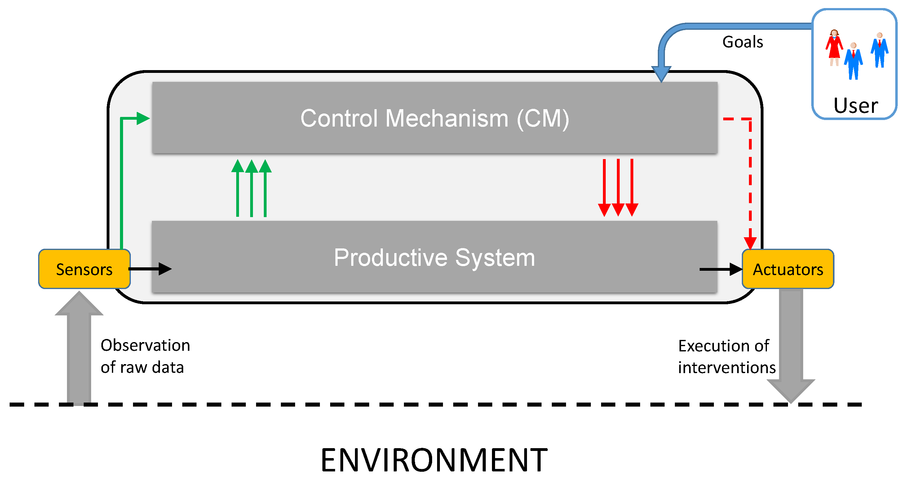
This position paper is based on initial work presented in [11] and provides a first concept for answering these questions. It describes a measurement framework for quantifying a degree of self-adaptation and outlines how this can be used to answer the questions about stability and an expected degree of self-adaptation. However, it is meant as a position paper that argues with the need for research effort and tries to outline a possible path into this direction—rather than providing a fully investigated solution.

The remainder of this article is organized as follows: Section 2 explains the underlying system model for SASO systems for clarification purposes and names the assumptions made by the authors. Section 3 briefly summarizes the state of the art in the field and derives the research gap that is addressed in this article. Afterwards, Section 4 presents a measurement approach and discusses next steps towards determining the stability and a context-dependent expected degree of self-adaptation behavior. Section 5 analyses the measurements in three simulation-based studies. Finally, Section 6 summarizes the article and gives an outlook on future work.

2. System Model

A system within this position paper is an entity that interacts with other entities, i.e., other systems, including hardware, software, humans, and the physical world with its natural phenomena. These other entities are referred to as the environment of the given system. The system boundary is the common frontier between the system and its environment.

We assume a SASO system S to consist of a potentially large set A of autonomous subsystems $a_i$. Each $a_i$ is equipped with sensors and actuators (both physical and virtual). Internally, each $a_i$ distinguishes between a productive system part (PS, responsible for the basic purpose of the system) and a control mechanism (CM, responsible for controlling the behavior of the PS and deciding about relations to other subsystems). This corresponds to the separation of concerns between System under Observation and Control (SuOC) and Observer/Controller tandem in the terminology of Organic Computing (OC) [12] or Managed Resource and Autonomic Manager in terms of Autonomic Computing [4]. Figure 1 illustrates this concept with its input and output relations. The user guides the behavior of $a_i$ using a utility function U and (normally) does not intervene at the decision level: Actual decisions are taken by the productive system and the CM. We model each subsystem to act autonomously, i.e., there are no control hierarchies in the overall system. Please note that for this context of this paper an explicit local configuration of the SuOC is necessary—which in turn limits the scope of the applicability of the proposed method.

At each point in time, the different productive part of each $a_i$ is configured using a vector $c_i$. This vector contains a specific value for each control variable that can be altered to steer the behavior, independently of the particular realization of the parameter (e.g., as reel value, Boolean/flag, integer or categorical variable). Each of these SuOCs has its own configuration space, i.e., an n-dimensional space defining all possible realizations of the configuration vector. The combination of the current configuration vectors of all contained subsystems of the overall system S define the overall configuration of S. We assume that modifications of the configuration vectors are done by the different $CM$ only, i.e., locally at each subsystem. The greater the difference between the last and the current instance of the configuration vector (e.g., expressed in terms of the Euclidian distance) or the more changes have occurred in an observation period, the greater the degree of self-adaptation behavior.

We do not restrict the system composition, i.e., we allow open systems [13]. Each $a_i$ can be controlled by different users and it may be designed and developed using arbitrary concepts. This includes that we are not aware of the strategies performed by $C{M}_i$, the goal provided by the corresponding user, and the applied techniques, for instance. However, we assume to be able to observe the external effects: (i) the actions that are performed by each $a_i$ and (ii) the messages that are sent and received. The actions performed by each $C{M}_i$ are assumed to be either related to changes in the structure or in the behavior, where the behavior is directly mapped to a re-parameterization of the productive part (the SuOC). Technically, a relationship between two subsystems represents a functional connection. This means that cooperation may be required to solve a certain task: as input-output relations, as the (mutual) exchange of information, or as a negotiation between a group of $a_i$, to name just a few. In all these cases, the interactions between subsystems take place which we map onto the concept of organization: $a_i$ are connected functionally with other $a_i$ and these connections are established and removed over time.

We further assume that establishing and changing relations in technical systems requires communication. For simplicity reasons, we model communication as sending and receiving messages via a communication channel. We require that the medium be shared, and messages are routed using standard communication protocols and infrastructure, e.g., using the Transmission Control Protocol/Internet Protocol (IP) tandem. Correspondingly, $a_i$ are uniquely identifiable (e.g., via their IP address). We assume that each message has an origin and a destination, and there are no fake messages (i.e., from an attacker with a modified origin field). We also require that all messages be visible and external origins of these messages such as the users can be identified. This is particularly necessary to avoid influences from external being responsible for steering the behavior of each $a_i$ and consequently for re-configuration.

3. State of the Art

The identification of abnormal self-organization and adaptation processes is crucial for understanding SASO behavior and its causes. Existing metrics to identify SASO properties are either highly domain-specific and hard to generalize or restricted to simple, small-scale models [14]. Only limited research effort has been spent on metrics to determine the effort and the benefit of adaptation in distributed collections of autonomous subsystems, see [15] for an overview. Examples include the relation between working and adaptation time, the availability of subsystems for task processing, and the performance of the overall system (i.e., the degree to which a certain goal is achieved). Kaddoum et al. [16] discuss the need to refine classical performance metrics to SASO purposes and present specific metrics for self-adaptive systems. They distinguish between “nominal” and “self-*” situations and their relations. For instance, they measure the operation time about the adaptation time to determine the effort. Some of the developed metrics have been investigated in detail by Camara et al. for software architecture scenarios [17]. Moreover, success and adaptation efforts and ways to measure autonomy have been investigated, see e.g., [18].

Besides adaptation of behavior, measuring self-organization is of particular interest, since self-organization refers to an adaptation of the system’s structure (e.g., in terms of connections, interactions, or relations between subsystems). Relevant for SASO systems are basic metrics such as an interaction metric (i.e., the number of state changes), a decentralized emergence detection metric (polling several random agents in the system over shifting periods), and a limited bandwidth recognition metric (manually identifying collective behaviors of a system and breaking them down into local agent features) [14,19,20]. These simple measurements come up with limited information about the general states and the causes of the observed behavior. In contrast, an approach by Deaton and Allen [21] is already focused on interactions in the system: It measures the complexity of a system by a change in the number of interactions within a given time interval. Further examples use Shannon’s entropy to measure self-organization as an increase in the amount of information needed to forecast the upcoming system behavior [22] or to determine a so-called “degree of self-organization”: A system that is stuck in an attractor within the state space is defined to be self-organized, since the system cannot reach other states any more [23]. In another work, self-organization is measured as a function of an attractor’s dimension within the underlying state space [24]. A very basic concept is to understand self-organization as a negative change of emergence, see [25]. Schmeck et al. proposed to measure self-organization based on the relation between control mechanisms and productive systems in the overall system [26]—which amounts to a kind of structural self-organization but neglects dynamics. Finally, two closely connected approaches to quantify self-organization behavior has been presented in [27,28,29]: Ref [27,28] describe an approach, where the changes within a graph representation of the overall SASO system with subsystems as nodes and interactions as edges are quantified between two subsequent measuring periods. On the other hand, Ref [29] defines a dynamic degree of self-organization using the same system model and the same measurement periods by comparing probability distributions of generative models encoding the communications among the subsystems as interactions using divergence measures such as the Kullback–Leibler divergence. In this article, we will follow an attempt that resembles some of the ideas of the second approach.

In [30], some measurement aspects are mentioned which are necessary for control strategies of SASO systems. However, there is no integrated measurement framework for quantifying the behavior of SASO systems available, e.g., as the basis for comparing different approaches. Especially approaches to determine a “normal” or “appropriate” degree of adaptation for a certain situational context is missing.

Furthermore, there are several attempts to measure emergence in technical systems. By intuition, the term “emergence” refers to properties of a large-scale system consisting of autonomous processes or entities that appear at a macro-level and are not present at the micro-level (i.e., in the individual processes or entities). However, there is no commonly accepted definition of emergence and, consequently, the different measurement attempts follow varying goals. In the context of this paper, we consider emergence as the formation process transforming disorder into order based on self-organization (according to [3]).

Examples for measurement techniques include the following: Shalizi presented an approach that is based on the efficiency of predictions and makes use of approaches known from the domain of information theory [31], a closely related approach has been presented by Prokopenko et al. in [32]: In general, both aim at assessing which level (i.e., from micro to macro) is more efficient for predicting the next states. Similarly, Holzer and De Meer compare the information at the system level (i.e., the sum of all edges in a network-based representation) with the information of a lower level (i.e., a single edge in a network-based representation) [33]. As a result, emergence values are high for those systems with many components depending on each other and low for those systems that mostly comprise independent components. However, this is closely related to the concept of self-organization as outlined above. As an alternative, the Organic Computing domain used Shannon’s discrete entropy measure as a basis for defining emergence. The authors modelled all relevant attributes of the system as random variables and determined emergence as a decrease of entropy based on self-organizing processes [34]. This has been extended towards continuous attributes in [35] by deriving probability distributions of attributes and comparing them using divergence measures. In this article, we propose a similar approach for measuring self-adaptation.

The previous discussion highlighted that there is no integrated and unified framework for quantifying properties of SASO systems. On the contrary, sometimes conflicting definitions and approaches prevent a generally accepted framework based on a common mathematical framework. This article aims to lay the foundation for such a framework by building on some of the previously described approaches (including [35] for emergence and [29] for self-organization). We further showed that there is currently no attempt to quantify the basic concept of self-adaptation, which is addressed by this article.

Finally, there is only a very limited number of contributions on when (and if at all) to adapt in the literature. One quite young example is [36], where the authors make use of a metaphor called ’technical dept’. The basic idea here is to introduce a gate that either enables or disables the adaptation mechanism. This decision is based on deriving an integrated score for defining the current so-called ’temporal interest’ and the expected ’revenue’. Although this is an interesting first step into the research direction outlined in this paper, it differs significantly from the basic idea postulated here: It tries to find a balance between given key indicators rather than taking stability and user acceptance into consideration. It further does not provide a measurement for external analysis that quantifies a suitable amount of adaptation decisions.

4. Quantification of Expected Self-Adaptation

As outlined before, there is a reasonable amount of work trying to quantify the degree of self-organization in an overall SASO system. However, the observable effects of SASO mechanisms manifest also in modifications of the behavior of subsystems that are subject to a modifiable configuration. We propose to develop a measurement framework for quantifying the degree to which a SASO (sub-)system changes its behavior in a given observation period. With such a technique at hand, the system can quantify the heterogeneity of configurations, e.g., in response to dynamics of the environment or external disturbances, and consequently assess the impact of an adaptation. Such a measurement comes with a second advantage: It can be used to compare SASO systems under identical conditions to analyze which solution requires higher adaptation effort and achieves stable solutions faster.

In addition to the system model from Section 2, we require that the current configuration of a subsystem must be accessible. We, therefore, assume that each subsystem provides a self-description in terms of its variable control parameters (i.e., the connection between CM and productive system as indicated by the red arrows in Figure 1) and their current configuration, possibly together with a description of boundaries (i.e., maximum and minimum values, update resolution). Please note that we still do not need access to the internal decision processes, goals, and preferences of the individual subsystem.

In the following section, we initially define challenges that need to be addressed towards such a measurement framework. Afterwards, we define the first approach for such a measurement framework by addressing aspects of the first derived challenges. This approach makes use of generative probabilistic models, which are defined in this context.

4.1. Challenges for Defining a Measurement Framework

In the following paragraphs, we define challenges that need to be addressed towards a measurement framework for self-adapting systems. We assume that self-adaptation manifests itself by means of configurations that are altered through internal decision mechanisms. We further assume that this actual configuration of all parameters relevant for controlling the productive behavior of a subsystem is accessible through interfaces. Consequently, each subsystem $a_i\in S$ has a current configuration $c_i\in C_i$.

Challenge 1: Quantification of changes

We assume that a subsystem $a_i$ does not need to modify its configuration if all conditions are stable. This implies that any adaptation is a response to environmental dynamics, reorganization effects, or disturbances. Conceptually, we model each subsystem $a_i$ as a process that generates observable samples (i.e., configurations). We further model the observation process as a snapshot of all configurations $c_i$ that is processed with a pre-defined sampling rate. In a first approach, we may quantify the change statistically by accumulating the number of observed changes. The advantage of this approach is that it is easy to compute. This requires research on the following questions: (a) Which size of the sampling interval $d_{adaptation}$ is appropriate for measuring self-adaptation? (b) How does the proposed measurement behave if being used as a basis for comparisons between different self-adaptation mechanisms? and (c) If configurations possibly cover a continuous space, they have to be discrete in the first place—how does such a pre-processing affect the measurement?

Challenge 2: Heterogeneity of changes in the subsystems’ configurations

The outlined approach has the disadvantage of not incorporating the heterogeneity of configurations within the system during the observation period. This means that only the change itself is considered, but not the variety of different configurations and the diversity of observed adaptations. In this sense, the previous approach provides just an easy-to-compute indicator for the adaptation behavior but neglects detailed descriptions of the behavior. To overcome these limitations, we propose to consider the frequencies and heterogeneity of the adaptations. Expressed in a probabilistic framework, we represent each subsystem $a_i$ as a process that generates observable samples (i.e., configurations). We assume an observation period of a given length in which actual configurations of all contained subsystems are collected in a certain sampling frequency. When measuring the degree of self-adaptation from the outside (e.g., without access to the internals of the $a_i$), we either use the configurations as they are, use pre-processing techniques to extract the values of attributes (features) from samples (observations), or use a hybrid approach.

Based on this idea, we define the degree of self-adaptation as an unexpected or unpredictable change of the distribution underlying the observed samples (i.e., the configurations). We propose to measure the expected amount of information contained in a new distribution concerning for a reference distribution of samples by using divergence measures (e.g., the Kullback–Leibler divergence [37]): The higher the difference between both distributions, the more self-adaptation took place. Compared to the concept outlined in Challenge 1, the probability distributions have the advantage that they take all occurred configurations into account. For instance, switching only between two different configurations will result in a lower degree of self-adaptation than taking on highly diverse configurations, while the static degree will only recognize the various changes. The basic challenge here is to compare the different divergence measures and change detecting techniques known in the machine learning domain and determine which provides the most reliable values for quantifying the severity of the change. Such a model requires also research on the following questions: (i) How to handle configurations that may consist of other variable types (e.g., including categorical or Boolean), and (ii) How to handle adaptations that may be done more frequently or are done asynchronously within S (as a result of isolated decisions by each $a_i$, negotiated adaptations, or chain reactions, for instance).

Challenge 3: Stability of self-adaptation processes

The two previous challenges proposed to measure self-adaptation as a change in the configuration behavior of the contained subsystems. Conceptually, this is based on the assumption that self-adaptation is a response to certain events and influences (e.g., disturbances, outages, or environmental dynamics): To maintain a certain utility or to self-improve this utility over time, certain configurations are more beneficial than others in a particular context. However, this basic idea of self-adaptation also assumes that in case of static conditions (or only slowly changing situations) no adaptations are needed. Consequently, a self-adaptation process is assumed to result in stable and optimized solutions. A resulting challenge is then to develop techniques which can analyze this stabilization process in detail. This especially means techniques to identify cases where re-adaptation is not converging towards (optimal) behavior or runs into oscillating patterns.

The basic idea is illustrated in Figure 2: The green arrows indicate the comparison of probability distributions as discussed in the context of Challenge 2. We define periods of consecutive estimations and compare the results of the measurements as aggregated value for a certain time frame ($T_{Stability}$) against the previous time frame. Therefore, $T_{Stability}$ specifies the size of the considered window and d refers to the fixed/sliding window size. In particular, we now shift the focus towards long-term comparisons instead of the one-by-one comparisons. Again, a suitable approach may be the usage of a hybrid technique, i.e., considering both windows: an initial pre-defined window and the previous sliding window. From this general concept, the following research questions have to be addressed: (a) What is a meaningful lower bound for a factor k (number of frames) such that $T_{stability}=k\ast d$ provides meaningful results for a stability estimation? (b) How can the stability be expressed to consider the differences between the observed behavior within different time frames (of size $T_{Stability}$)? and (c) How can we distinguish between a short-term level of stability (i.e., k is 1—in response to an identified disturbance using techniques such as [38]) and the long-term stability of the system (i.e., k is larger than 1—taking certain interval into account, such as a day)?

Challenge 4: Sliding windows

The probability-based approaches outlined before require inherent comparability of two probability distributions. Transferred to the temporal behavior of a SASO system, this implies that the potential adaptation process manifests itself in the difference between a current and a referential distribution of attribute occurrences. For comparison, we must define that both measurement periods cover the same period. This can be done using a sliding window approach: A fixed period d is used to observe samples for the current estimation process (i.e., between time $t_0$ and $t_{-1}$) and the same duration is used for a reference observation (i.e., the period directly before the current observations are done: between $t_{-1}$ and $t_{-2}$). Alternatively, the reference window might be fixed (i.e., static), e.g., at the begin of the observation (here, slow changes can be detected easier, but changes the composition of S always require new reference models). Similar considerations have been presented in the context of measuring emergence in [35]. However, it may be beneficial to use a hybrid approach that combines both concepts: estimating the change compared to the previous period and against a static distribution to be able to cover all aspects. We propose to investigate the impact of choosing the window: (i) in terms of which period should serve as reference distribution, and (ii) how d has to be configured depending on the message frequency.

Challenge 5: Mutual influences among configurations

Until now we assumed that configurations are chosen independently from each other, and further assumed that the overall distributions can be approximated by Gaussians. However, both assumptions may not be entirely true in real-world conditions. For instance, there is a temporal dependency among configurations of an individual subsystem, since a configuration is selected in response to external conditions. These conditions typically develop rather than shifting abruptly. Consequently, subsequent configurations are typically ’similar’ based on a similarity metric covering the configuration space (i.e., Euclidian). Furthermore, the decision of an individual subsystem may also have an impact on the utility of a neighbored subsystem, and consequently on the decision about its next configuration. We call this concept ’mutual influence’ [10]. Especially when considering detected mutual influences in the self-adaptation mechanism as outlined in [39,40], the measurement of a degree of self-adaptation is directly influenced. This results in the challenge to incorporate these mutual influence information in the measure and in trying to distinguish between effects on the actual value of the measure, i.e., to which part did the acting in shared environments influence the actual value and to which part the basic self-adaptation mechanism? This can be augmented with information about correlations between configurations and their occurrence in distributions.

Challenge 6: Self-explanation of SASO behavior

Finally, the last challenge that takes all information from the previous challenges into account is dedicated to developing mechanisms for self-explanation. Given the possibility that we can quantify a degree of self-adaptation including a measure of stability, we can use this information to identify abnormally high adaptation behavior. This may be perceived as incomprehensible by users and consequently requires explanations. Consequently, several questions arise in this context: (a) How can we determine abnormally high adaptation behavior, possibly based on a certain context (i.e., situation)? (b) How can we identify root causes that triggered these adaptations? and (c) How can we generate comprehensible explanations for this behavior that are acceptable for users?

In this article, we present a first concept that proposes possible solutions for Challenge 2 and Challenge 4. We will outline this in the following paragraphs.

4.2. Measuring a Degree of Adaptation Based on Generative Probabilistic Models

We define self-adaptation as an unexpected or unpredictable change of the distribution underlying the observed samples (i.e., the configurations of the subsystems). Consequently, a divergence measure can be applied to compare two density functions. We will refer to a density function $p(x)$ representing an earlier point in time and to $q(x)$ as a density function representing the current observation cycle. A famous divergence measure is the Kullback–Leibler (KL) divergence $KL(p||q)$ (also called relative entropy), see [37]. It is defined for continuous variables as follows:

$$KL(p||q)=-\int p(x)ln\frac{q(x)}{p(x)}dx$$

(1)

The advantage of $KL$ is that it fulfils some important requirements: (1) if $p(x)=q(x)$ the measure $KL(p||q)$ is 0, and (2) $KL(p||q)\ge 0$. Reformulating Equation (1) results in:

$$KL(p||q)=-\int p(x)lnq(x)dx+\int p(x)lnp(x)dx$$

(2)

The formula can be interpreted as follows: It measures the expected amount of information contained in a new distribution concerning a reference distribution of samples. However, KL is not symmetric which means that it comes up with different results depending on which of the two distributions we use as reference and which as a comparison. We can easily turn it into a symmetric variant as follows:

$$K{L}_2(p,q)=\frac{1}{2}(KL(p||q)+KL(q||p))$$

(3)

Based on this symmetric variant, we can reformulate Equation (2) as a symmetric variant as follows:

$$\begin{array}{c}\hfill \begin{array}{c}\hfill K{L}_2(p,q)=\frac{1}{2}(KL(p||q)+KL(q||p))\\ \hfill =\frac{1}{2}(\int p(x)lnp(x)dx-\int p(x)lnq(x)dx\\ \hfill +\int q(x)lnq(x)dx-\int q(x)lnp(x)dx)\end{array}\end{array}$$

(4)

We propose to use Equation (4) as a measure for quantifying self-adaptation processes. The basic idea is that the measure increases if the two distributions begin to change. This increase is a result of comparing the distributions of the observed samples, or more precisely, of the distribution of densities of the observed samples within the input space during a certain time interval. The more subsystems $a_i$ adapt their configuration due to changing conditions, the higher is the divergence to the previous distribution. As a result, the measure will indicate a higher degree of self-adaptation.

In comparison to other possible measurement techniques, this approach is characterized by a set of advantages:

• In comparison to approaches following the concept of measuring autonomy as outlined, e.g., in [26], our method does not rely on a static encoding of possible configurations pre-defined in number of bits.
• In comparison to approaches using the discrete entropy (e.g., outlined for measuring emergence in [34]), it is continuous and does not rely on binning (which introduces more parameters and a certain bias).
• It is independent of the notion of other concepts such as self-organization or emergence.
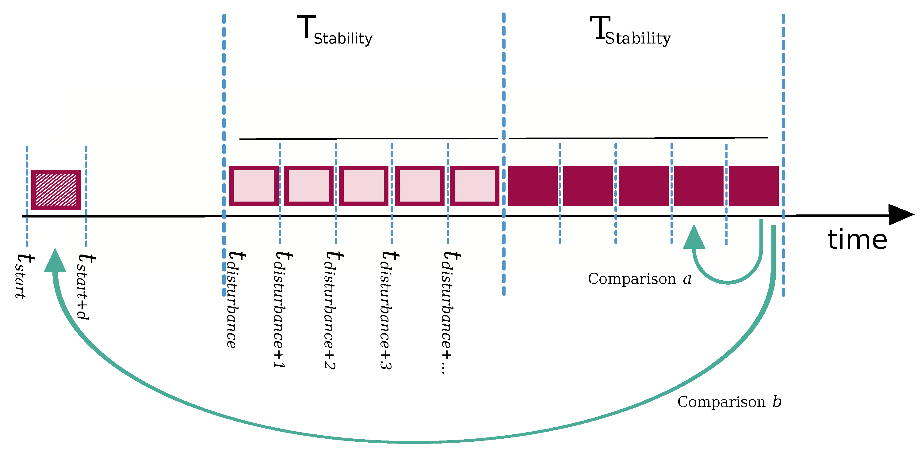
• Although it makes use of measurement period (windows), it is continuously applied. It does not need a trigger (e.g., the detection of a disturbance as used [27], for instance).
• It does not require a model of the internal decision processes of the autonomous subsystems $a_i$, since it just considers the externally visible configuration settings.
• It can easily be applied to, e.g., hierarchical structures of SASO systems in terms of considering only those subsystems $a_i$ that belong to a certain authority.

Although KL comes with some limitations (e.g., the absolute value is hard to interpret), it fulfils the most urgent requirements we formulated for measuring a degree of self-adaptation:

• It is zero if both distributions (i.e., derived from the reference and the current observation period) are identical. This means that the same configurations are observed. Theoretically, there may be switches between different agents running the configuration of the other one and vice versa, but in general this is a reliable approximation for constant behavior.
• In turn, high values of KL indicate strong changes in the configurations of the contained subsystems. This indicates a high degree of self-adaptation.
• A major issue in this context is that the values of KL highly depend on the considered feature vector (i.e., the number, the type, and the resolution of the configuration parameters) as well as the frequency in which adaptations are done. These values are highly application-dependent. However, the comparison is always made within the domain—meaning that the ordering is correct, but the individual actual value does not much about the severity of the change. This can be defined in relation to a set of observations, i.e., based on experiences with the application under investigation. This leaves the question open how to determine a real ’level’ out of the KL values.

5. Use Cases and Evaluation

To analyze the behavior of the measurement framework as defined above, we selected three different use cases: urban traffic control based on our preliminary work, the publicly available swidden farming model. and situation-aware parameterization of data communication protocols. The rationale behind this choice was to identify three completely different scenarios (in terms of application and configuration parameter definition) for analyzing the characteristics of the measurement values. In future work, we will consider further scenarios including artificial simulations that show pre-defined behavior.

For all scenarios, we initially describe the (simulated) systems, followed by an overview of the observed configuration parameters that are subject to self-adaptation. Afterwards, we analyze the behavior of the measurement framework in details. The section is concluded by a discussion of the characteristics summarizing both scenarios.

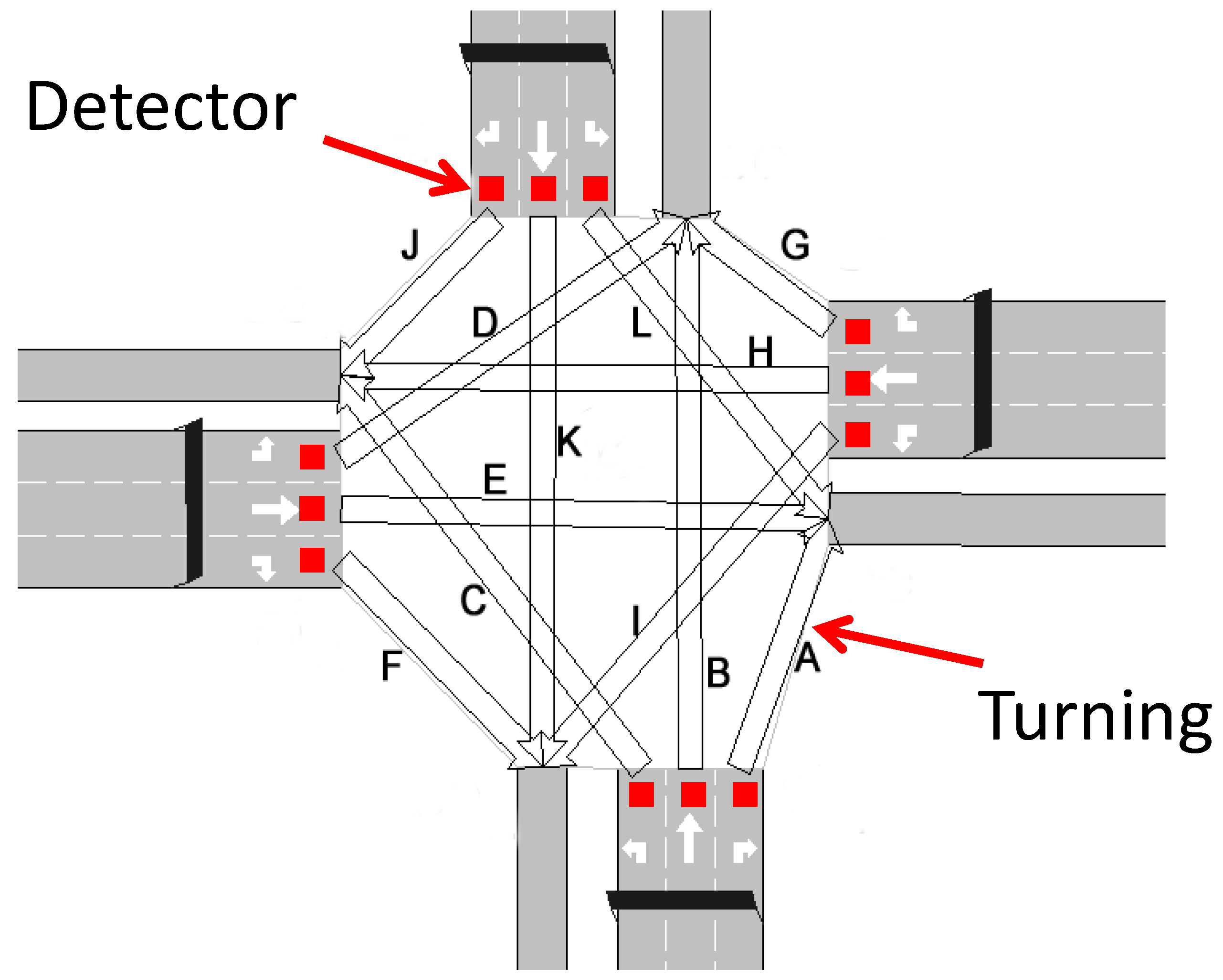
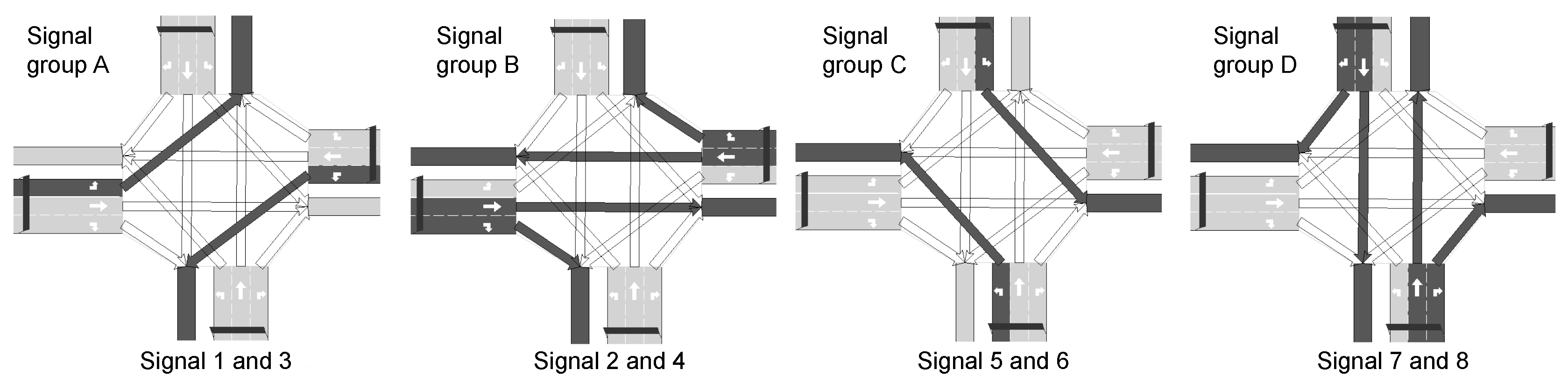
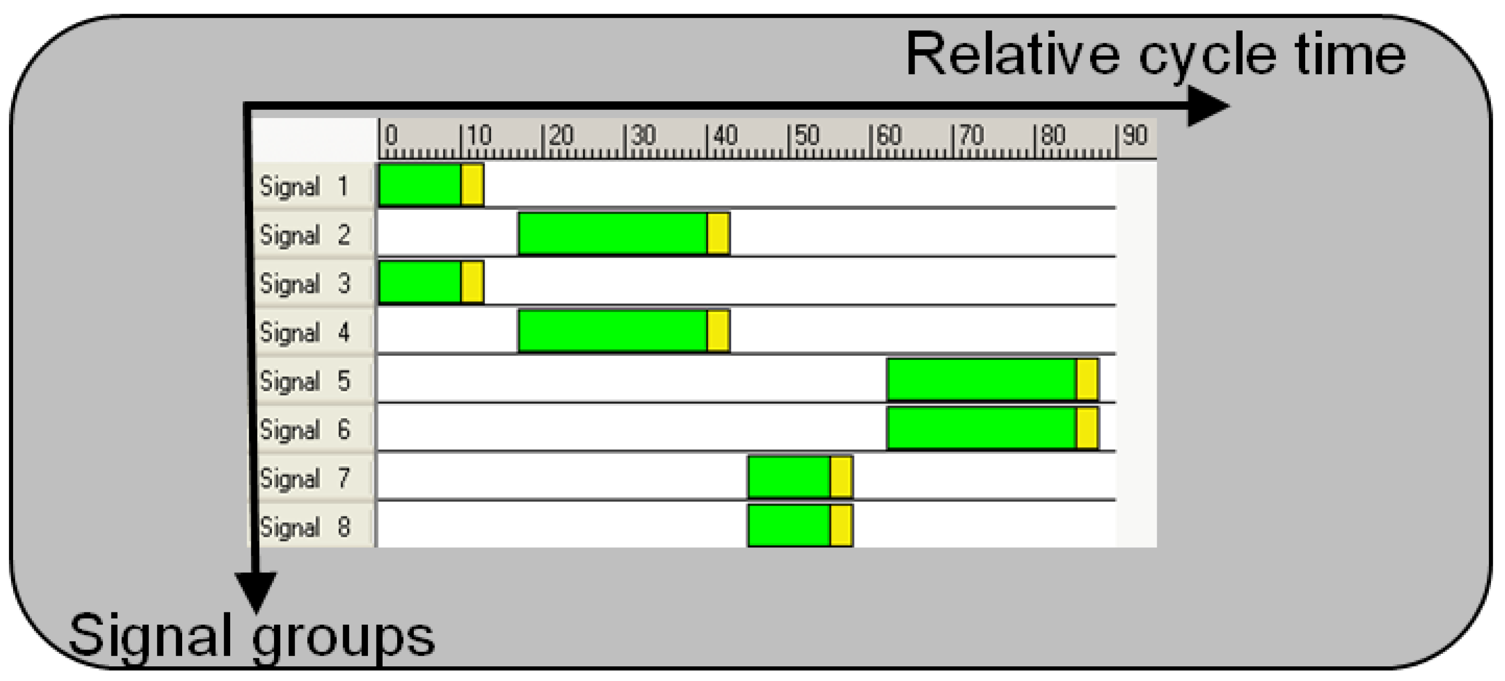
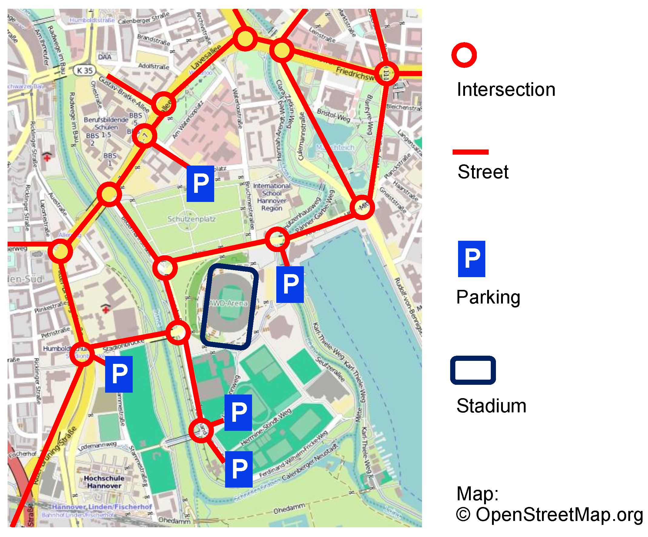
5.1. Application 1: Traffic Control

Traffic control at urban intersections is used as a second scenario for evaluation purposes. Urban traffic networks are a promising application domain for SASO systems since traffic is highly dynamic and volumes rise constantly in cities and on highways worldwide. Consequently, there is a need for situation-dependent self-adaptation. One successful representative of such a self-adaptive traffic control system is the “Organic Traffic Control” (OTC) system [8,41]. OTC is based on the Observer/Controller model [12] as known from the domain of Organic Computing [3] and learns the best traffic control strategy at an urban intersection a runtime. In general, OTC consists of three major components: (1) autonomous learning of self-configuration strategies for traffic lights (i.e., duration of green times at each intersection) [42], (2) self-coordination to establish Progressive Signal Systems (PSS) [43], and (3) negotiation to derive route recommendations following Internet-based protocols [44]. In the context of this article, the aspect of self-adaptation in terms of configuring green duration of phases are of particular interest.

5.1.1. Parameters

The four-armed intersection shown in Figure 3 consists of four approaching and four leaving sections. The intersection’s topology is defined by the turnings between these sections. Each turning might be signalized by its traffic light or it might share a traffic light (e.g., turnings for straight-ahead and turn-right). Usually, detectors are installed at each turning to determine the traffic stream volumes based on occupancy signals (e.g., realized as induction-loops in the street surface).

Those turnings with non-conflicting traffic streams are used to form signal groups (see Figure 4). Based on these signal groups, the signal plan can be defined. Consider the signal plan in Figure 5 that shows the duration of green and yellow periods for signal groups A to D from Figure 4. At other times, the so-called interphases, all traffic lights show red to avoid accidents with conflicting streams. Together, the green, yellow and red periods define the cycle time. After completing a full cycle, the signalization starts again. For coordination purposes, intersection controllers of neighbored intersections with the same cycle length can be synchronized by determining an “offset”, i.e., a relative start of the synchronized phase within the cycle.

Consequently, the controllable parameters for self-adaptation in this scenario are the green durations of all contained signal groups.

5.1.2. Experimental Setup

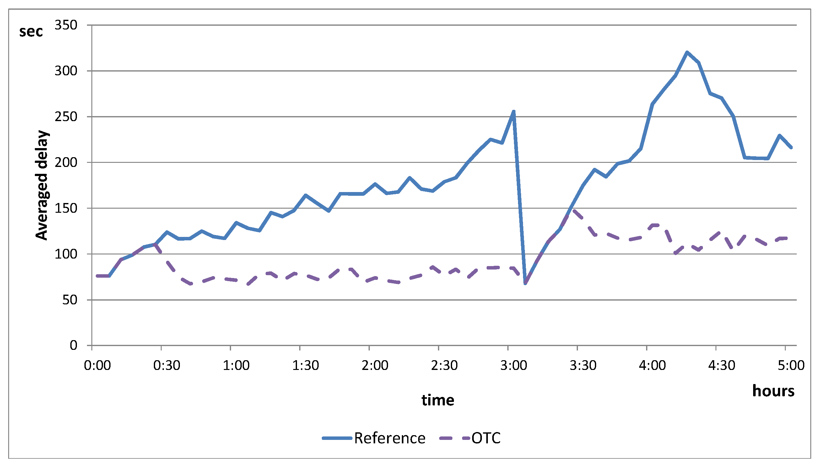
The evaluation of the OTC scenario is based on a simulation of a stadium event in the city of Hannover, Germany, which generates abnormally high approaching and departing traffic. As a result, we expect increasing adaptation effort of the individual intersection controllers when the approaching traffic for the stadium event is increasing the ’normal’ traffic volumes. Figure 6 shows the simulated part of Hannover’s street network, which is modelled within the professional traffic simulation toolkit ’Aimsun Professional’ [45]. The signal plans and the traffic data are based on information provided by the responsible authorities, i.e., the Landeshauptstadt Hannover (Fachbereich Tiefbau, Bereich Koordinierung und Verkehr) and the Verkehrsmanagementzentrale Niedersachsen (Region Hannover). The traffic data has been obtained from a census performed on 9 May 2009. The Aimsun models reflect the topology of the intersections and roads as of spring 2010. Since the topology of the road network did not change within this period, the combination of both is possible. The signaling of the traffic network surrounding the stadium is part of the overall traffic strategy for the urban area of Hannover.

In reality, the intersection controllers are operated by seven different daytime-depending strategies: five according to a classification of days (Monday has its class as week start, Tuesday to Thursday are considered to be one class as they are ’normal’ days, Friday is an own class as the end of the week, Saturday is an own class as half working day, and Sunday is an own class as work-free day—bank holidays are considered to be well). Furthermore, the control strategy contains two cases especially designed for stadium events and cover the approaching and departing traffic. We focus on this scenario in our evaluation. In general, the approaching strategy optimizes the network’s throughput on the main streets approaching the stadium, while the departing one provides traffic’s fast departure of the inner-city region. These two strategies serve as a reference solution for the OTC solution.

The simulation is performed—as mentioned before—using the traffic simulation toolkit Aimsun NG Professional [45]. Aimsun is an abbreviation for “Advanced Interactive Microscopic Simulator for Urban and Non-Urban Networks”. The simulator is an integrated transport modelling software, developed and licensed by Transport Simulation Systems (TSS) from Barcelona, Spain. In general, professional microscopic traffic simulators such as Aimsun are simulation tools that aim at emulating the flow of individual vehicles through urban road networks as realistically as possible. To capture the full dynamics of time-dependent traffic phenomena, a large part of current microscopic traffic simulators rely on the theory of car-following, lane changing and gap acceptance models to model the particular behavior of vehicles. Therefore, both global and local phenomena have influence on the individual vehicle’s behavior—details on the theoretical parts are, e.g., given in [46]. Traffic engineers of authorities make heavy use of these simulators to plan and optimize the traffic control strategies and topology of intersections in cities worldwide.

5.1.3. Evaluation

The evaluation of the OTC scenario consists of two parts: Initially, we demonstrate that the self-adaptive and self-learning strategy performed by OTC improves the traffic behavior in comparison to the existing (static) solution. We consider the main goal—average delays within the entire network—as a criterion. Afterwards, we introduce the self-adaptation measurement based on $K{L}_2$ as defined in Equation (4) and show how the measurement behaves.

Initially, we show that the OTC control (i.e., the self-adaptation) has been successful. Therefore, we analyze the metric ’average travel times’ for the entire network (which should be as low as possible) by comparing the results of simulating the reference signal plan as used in reality with simulating the OTC system that self-adapts the green duration of traffic signals in the network over time. Figure 7 shows the results. We can see that the self-adaptation strategy has been highly successful, since it decreased the average delays drastically.

In a next step, we investigate how the $K{L}_2$ measure behaves as an indicator for a degree of self-adaptation. Therefore, we introduce sliding windows again. Here, we consider a 30 min interval as window size: We searched for the smallest feasible window size, and shorter windows resulted in too fewer samples to be covered for deriving a meaningful distribution (and consequently for the density estimation).

Initially, we simulate another 30 min to determine a reference distribution of configurations. In general, each intersection controller has to perform the currently active configuration for at least two full cycles due to safety (switches are only allowed to the end/beginning of a cycle) and learning reasons (assessment of the success of a rule requires feedback that is the result of analyzing the effectiveness of the rule). Typically, a cycle is about 60 to 100 s. Considering these restrictions, each intersection controller can in maximum have 15 different configurations per window of 30 min. Depending on the dynamics of the traffic conditions and the traffic volumes (the higher the volume, the longer the cycle time), the average number of adaptations is between almost 0 (static traffic behavior) and about 22 changes in the configuration, not considering that this potentially includes switching back to one of the previous configurations (i.e., not considering the diversity of the configurations).

Table 1. Results of the $K{L}_2$ measure in the OTC example: Comparison of the distributions against the no-stadium traffic distribution generated in a separate run. The index i in $p_i(x)$ indicates the end of the 30 min window.

${\mathit{p}}_{30}(\mathit{x})$	${\mathit{p}}_{60}(\mathit{x})$	${\mathit{p}}_{90}(\mathit{x})$	${\mathit{p}}_{120}(\mathit{x})$	${\mathit{p}}_{150}(\mathit{x})$	${\mathit{p}}_{180}(\mathit{x})$	${\mathit{p}}_{210}(\mathit{x})$	${\mathit{p}}_{240}(\mathit{x})$	${\mathit{p}}_{270}(\mathit{x})$	${\mathit{p}}_{300}(\mathit{x})$
$326.7$	$417.6$	$555.6$	$543.8$	$812.2$	$829.2$	$5913.8$	$876.9$	$769.8$	$804.1$

lists the results. It shows the values for calculating the $K{L}_2$ measure of each distribution determined for a 30 min window in comparison to the ’normal’ self-adaptation behavior determined in a separate run of the simulation (also taking a window of 30 min into account). Considering the values given in Table 1 for the OTC strategies using the different windows, we can see the desired effect. Initially, there is ’normal’ traffic, which is covered by a few adaptations in the network. As soon as the traffic volumes that approach the stadium are starting to increase, the values for $K{L}_2$ indicate an increase of adaptation effort as well. The highest difference between subsequent distributions of configurations can be observed as soon as the traffic volumes start to depart from the stadium site. The reason is that the configuration now differs stronger from the previous ones, since opposing streams need to be preferred.

For the reference solution, the $K{L}_2$ measure results in values of $0.0$ for all considered windows besides one. This is because it follows a static strategy without changing the configurations of the intersection controllers. The only exception is at simulation time 3:00 h, where the switch between arriving and departing traffic is performed. This corresponds to the maximum values identified for the OTC strategy from Table 1.

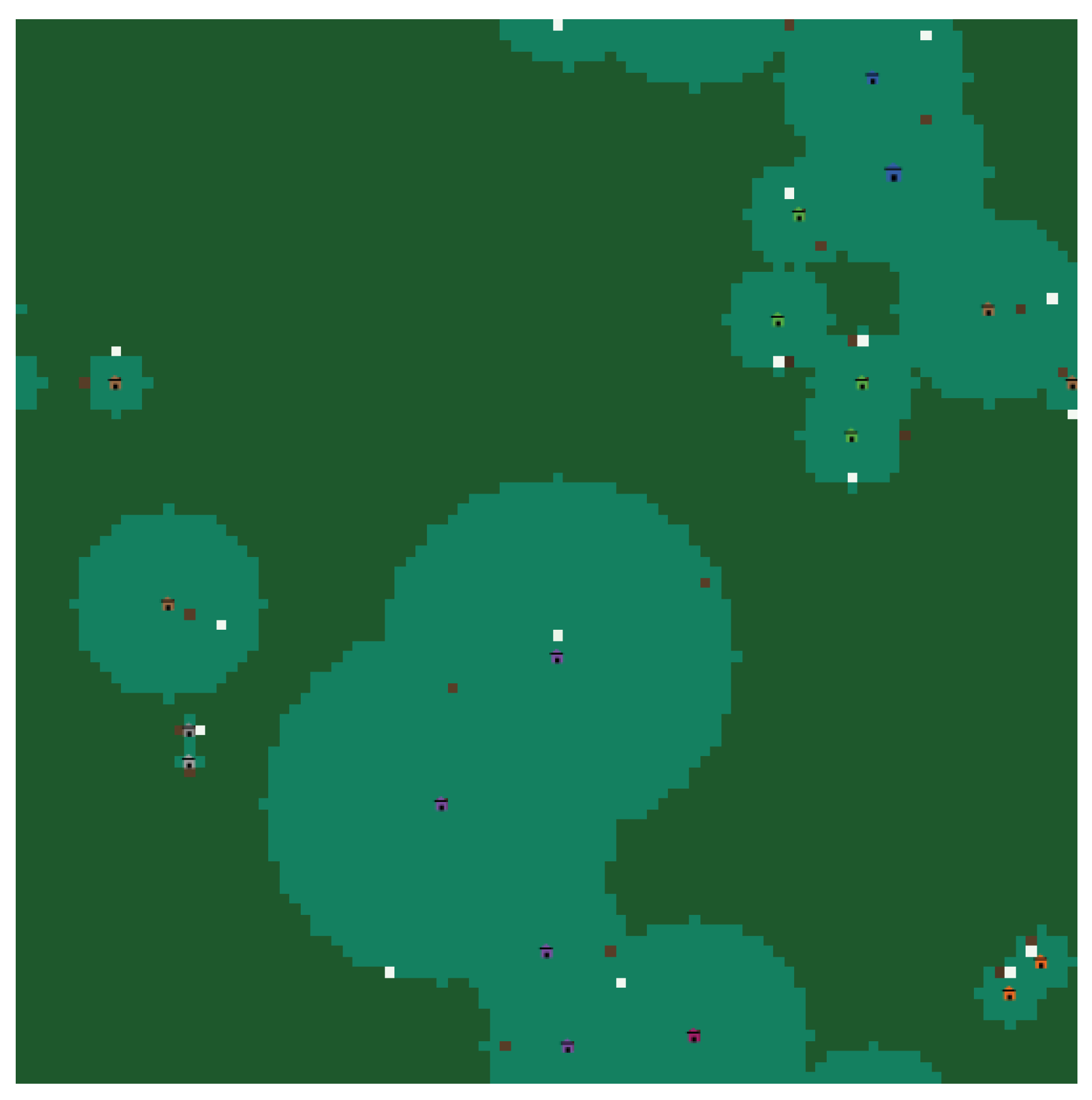
5.2. Application 2: Swidden Farming Model

As another scenario for analyzing the adaptation behavior at runtime using the metrics defined in the previous section, we use an existing simulation from the state of the art that considers human societies and how they interact with the bio-physical world. The “Swidden Farming” model [47] simulates the behavior of farming households as agents using slash-and-burn agriculture to farm a specific field. These fields are called “swidden”. The basic idea of this simulation is to explore how the individual households (or farmers) adapt their behavior according to the dynamics of a continuously changing environment. These dynamics are characterized by aspects such as harvest return, farming costs, and soil fertility loss. Furthermore, the simulation is used to explore the impacts of a set of social or economic decisions associated with farming. This includes, for instance, questions such as: How can potential costs and benefits for choosing land be evaluated and when should a particular piece of land with low productivity be distracted. Households are modelled as an evolution process: They reproduce successors and consider land residence rules. Figure 8 shows a screenshot of the simulation.

5.2.1. Parameters

To allow for self-adaptive behavior, the simulation contains a set of parameters that are adapted. The farming strategies of the household agents are associated with five configuration variables listed in

Table 2. Parameters of the swidden farming model.

ID	Parameter Name	Description	Parameter Range
1	move-dist	The distance an agent moves if it must find a new	[1;5]
		location for its farmstead.
2	move-threshold	The households moves to a new unoccupied area if	[0;1]
		its energy level drops below this threshold.
3	fission-rate	Amount of energy needed to reproduce a new household	[1;2]
		Defined about the initial household energy.
4	farm-dist	Maximum distance an agent will travel to a farm	[1;20]
		Radius of area a farmstead claims ownership, if
		this is not already occupied by another farmstead
5	min-fertility	Minimum fertility of a patch for being considered	[0;1]
		as next farmstead location.

. The table contains these parameters, briefly explains their impact, and names the range in which the parameters are controlled. The resulting configuration of each farmer agent steers its behavior in the system. The farmer agents interact with each other and make independent decisions on where to farm, taking their past and current actions into account for adapting to the environmental change and maximizing farming returns as well as minimizing the distance of travelling from farmstead to field. Details of the process are given in [47].

Self-adaptation manifests itself in this model using agents deciding on how to farm. Therefore, the parameters given by Table 2 are manipulated over time. Consequently, we measure the adaptation process in terms of observing the change of agriculture strategies of agents controlled—which again is defined as changing these modifiable configurations. There is another parameter—energy—that is not directly controlled by the agents and hence not part of the configuration vector. This value describes the current state of the agent and is therefore taken into consideration for evaluation purposes.

5.2.2. Experimental Setup

The swidden farming model is implemented in NetLogo [48]. Simulations are performed with the basic setup and dynamics provided by the author of the model ( Simulation is freely available at https://www.comses.net/codebases/3826/releases/1.3.0/ (last access: 24 October 2019)). We did not change any parts of the implementation and just used it as a reference model [47] since we are not interested in optimizing the model but in analyzing the self-adaptation behavior. In particular, this means to keep the standard values as follows: the ’innovation rate’ is set to $0.1$ and the ’bad year’ value is set to 20.

To be able to apply the sliding window technique, we assume that each window has a fixed length with 200 time steps. Again, we aimed at finding a minimum window size that is suitable for the calculation of the probability distributions (or better: of the density estimation).

5.2.3. Evaluation

In contrast to the OTC scenario described in Section 5.1, we now must deal with a variable number of agents (or subsystems). Based on their success and the corresponding ’energy’ level, agents have a higher probability to generate offspring. This has an impact on the measurement of self-adaptation using our method: The more agents are simulated, the more configuration vectors are considered. Consequently, we assume stronger changes whenever the next generation is taking over. To demonstrate the effect, we initially show the development of the number of agents in the simulation. Figure 9 illustrates the results. We can see that initially there is a strong increase, which converges to values around 100 (with a deviation of $\pm 20$).

As a second aspect, we are interested in the frequencies of configurations. Figure 10 shows the different discrete instances of each configuration parameter together with the corresponding frequencies (i.e., the number of occurrences within a simulation run of 1000 steps). Values are available for each step of the simulation, i.e., each of the frequency counts sums up to 1000. We can observe that some parameters tend to be set to a limited set of values (e.g., farm-dist and move-threshold), while others better use the available spectrum. However, this does not say anything about the severity between the switches—and the number of changes in total. It just provides an indicator of the expected values for configurations.

Finally, we apply the $KL$ measure to investigate the behavior of our metric.

Table 3. Results of the KL measure.

Distribution	Reference Distributions		Current Distribution
	${\mathit{p}}_{\mathbf{1}}(\mathit{x})$	${\mathit{p}}_{\mathbf{2}}(\mathit{x})$	$\mathit{q}(\mathit{x})$
$p_1(x)$	$0.0$	$745,363.96$	$627,723.08$
$p_2(x)$	$114,059.83$	$0.0$	$115,678.78$
$q(x)$	$\mathrm{161.573.15}$	$173,359.67$	$0.0$

shows the results for using the basic, non-symmetric variant of $KL$, while

Table 4. Results of the $K{L}_2$ measure.

Distribution	Reference Distributions		Current Distribution
	${\mathit{p}}_{\mathbf{1}}(\mathit{x})$	${\mathit{p}}_{\mathbf{2}}(\mathit{x})$	$\mathit{q}(\mathit{x})$
$p_1(x)$	$0.0$	$429,711.90$	$394,648.12$
$p_2(x)$	$429,711.90$	$0.0$	$144,519.23$
$q(x)$	$\mathrm{394.648.12}$	$144,519.23$	$0.0$

shows the results of the symmetric variant. We can observe that there are significant differences between the sampling periods ($p_1(x)$ and $p_2(x)$) and the reference distribution ($q(x)$). We computed all combinations of distributions and provide the values. We can further see that the symmetric variant of $K{L}_2$ performs exactly as desired: It does not matter anymore which distribution we use as reference and which as sampling period since both directions come up with the same values.

5.3. Application 3: Organic Network Control

Data communication in distributed communication networks serves as a third scenario for evaluation purposes. Communication networks are a promising application domain for SASO systems, since data traffic is highly dynamic and the network itself consists of a potentially large set of autonomous subsystems (i.e., routers, switches, gateways) [49]. Time-dependent and event-triggered usage as well as the open structure (i.e., nodes join/leave and change their communication pattern continuously) call for a situation-dependent self-adaptation. One successful representative of such a self-adaptive network control system is the “Organic Network Control” (ONC) system [50]. ONC is based on the Observer/Controller model [12] as known from the domain of Organic Computing [3] and learns the best control strategy of an autonomous device within such a communication network. In particular, ONC has been successfully applied to the control of nodes in mobile ad-hoc networks [51,52], nodes in wireless sensor networks [50], hardware antennas [53], cellular networks [54,55], and cooperative optimization of end-to-end communication links using the example of TCP/IP [56]. In the context of this article, we rely on the use case of mobile ad-hoc networks.

5.3.1. Parameters

As a use case for ONC controlling a protocol of the mobile ad-hoc networks domain, we chose the Reliable Broadcast Protocol (R-BCast) as introduced in [57], since this protocol is representative for the research field of reliable broadcast protocols in MANets and provides a very basic mechanism. To achieve reliability and increase the packet delivery ratio compared to other protocols, additional effort is made by equipping the nodes with extra buffers. These round-robin-based buffers are used to store the last p unique packets the particular nodes received. In contrast to other protocols, the R-BCast protocol has significantly more variable parameters and consequently the task to control the protocol is more complex, but it also offers a higher potential benefit due to a dynamic adaptation.

Table 5. Variable parameters of the R-BCast protocol.

Parameter	Standard Configuration
Delay	$0.1s$
AllowedHelloLoss	$3messages$
HelloInterval	$2.0s$
$\delta$ HelloInterval	$0.5s$
Packet count	$30messages$
Minimum difference	$0.7s$
NACK timeout	$0.2s$
NACK retries	$3retries$

lists the parameters with their particular standard configuration; a vector containing a particular value for each of these parameters comprises the configuration of each entity at each point of time. We briefly summarize the parameters as follows: The delay variable is used to define the maximum deceleration time between receiving and forwarding a message. Due to the mobility in MANets, many protocols are built on exchanging “hello”-messages to keep track of their neighbors’ availability. Therefore, the R-BCast protocol has an AllowedHelloLoss variable defining the maximum of “hello”-messages, which may be lost until a neighboring node is assumed to be out of transmission range. Furthermore, the HelloInterval defines the duration between sending “hello”-messages, and the δ-HelloInterval randomizes this interval to avoid collisions. Besides managing a list of available neighbors, the protocol has a mechanism to hold broadcast messages in temporary storage—if a new node joins the sending distance, lists of the last n broadcasts (and not-acknowledged messages) are exchanged and missed messages are updated. Therefore, the Packet count parameter defines the number of messages in the temporary storage—the Minimum Difference defines the lowest border of the duration between two not-acknowledged messages to be handled as different broadcasts. The last two variable parameters are also part of this not-acknowledged (NACK) mechanism. These NACK messages are used to get missed broadcast messages. If a node has a broadcast message from Sender $S1$ with $ID4$ in its queue and receives a new one with $ID6$, it asks for the one with $ID5$ using a NACK message. In the process, NACK timeout defines how long the node waits for an answer for the NACK message until it repeats the process. NACK retries specifies how often the process is repeated. More details about the parameters and the process of the protocol can be found in [57].

5.3.2. Experimental Setup

The ONC framework is implemented in JAVA. The moving agents are simulated using the Multi-Agent Simulation Toolkit MASON [58], while the communication is simulated using the NS/2 simulation toolkit [59]. We reuse the scenario from [51,52]. In total, 100 agents have been created and applied to the simulated area, which has dimensions of 1000 × 1000 cells (i.e., corresponding to 1000 × 1000 m). The agents move according to a random-waypoint-model. The Physical/Mac layer is in IEEE 802.11 in ad-hoc mode at 2 Mbps. The scenario considers 10,000 s of moving and communicating agents, in which a total of $17,400$ broadcast messages are distributed. The learning component of the ONC system has been pre-trained in 10 runs with similar conditions (i.e., same simulation model, but different random seed) in order to have a populated rule-base and consequently an appropriate adaptation behavior of each node.

To simulate different conditions demanding for changes in the adaptation behavior, we change the simulation after 5000 s (i.e., $50\%$ of the simulated time): We start with 50 agents at begin of the simulation and add 50 more agents after 5000 s.

5.3.3. Evaluation

In contrast to the OTC scenario described in Section 5.1 and similar to the swidden farming model, we face a variable number of agents (or subsystems). We again increase the number of parameters—but even more challenging—we also increase the configuration space in terms of the number of possible values each parameter can have. This results in a significantly increased number of different parameter constellations.

The results in [51,52] showed that the ONC system can improve the utility function (which is a heuristic approximating the packet delivery ratio locally at each node). In this evaluation, we just focus on the behavior of the proposed measure for the quantification of self-adaptation. Again, we introduce windows (here: 2000 s each) and list the results of the $KL$ measure—

Table 6. Results of the $KL$ measure in the ONC example: Comparison of the distributions against reference distribution generated in a separate run with a pre-trained system (containing just the initial 50 agents). The index i in $p_i(x)$ indicates the end of the 1000 s window.

${\mathit{p}}_{2000}(\mathit{x})$	${\mathit{p}}_{4000}(\mathit{x})$	${\mathit{p}}_{6000}(\mathit{x})$	${\mathit{p}}_{8000}(\mathit{x})$	${\mathit{p}}_{10000}(\mathit{x})$
$11256.11$	$1602.13$	$3213.56$	$4437.18$	$4376.32$

shows the results.

Based on the values, we can observe two effects: On the one hand, all values are larger than in the other two scenarios. This is caused by the increased heterogeneity of the configurations and consequently the lower probably of observing exactly the same configurations for individual subsystems. On the other hand, we can see the expected behavior: As soon as we introduce more autonomous subsystems and correspondingly more configuration vectors that are compared within the two distributions, we face dramatically increased values of the KL measure. However, we can state that the desired effect of detecting and quantifying the change is visible already.

5.4. Discussion and Threats to the Approach

When considering the results of the three scenarios, we can observe a set of characteristics that allow for an assessment of the measure defined in Section 4.2:

• Considering the absolute values given in Table 4 and Table 1 we can see that the values themselves come without meaning. We cannot make any statement about the relation between the changes. In particular, the differences just show that there is a change or a stronger/smaller change, but statements such as “X is twice as strong as Y” are not possible.
• A better approach than $KL$ should come up with values that can be normalized to the standard interval $[0,1]$, since this allows for better comparability.
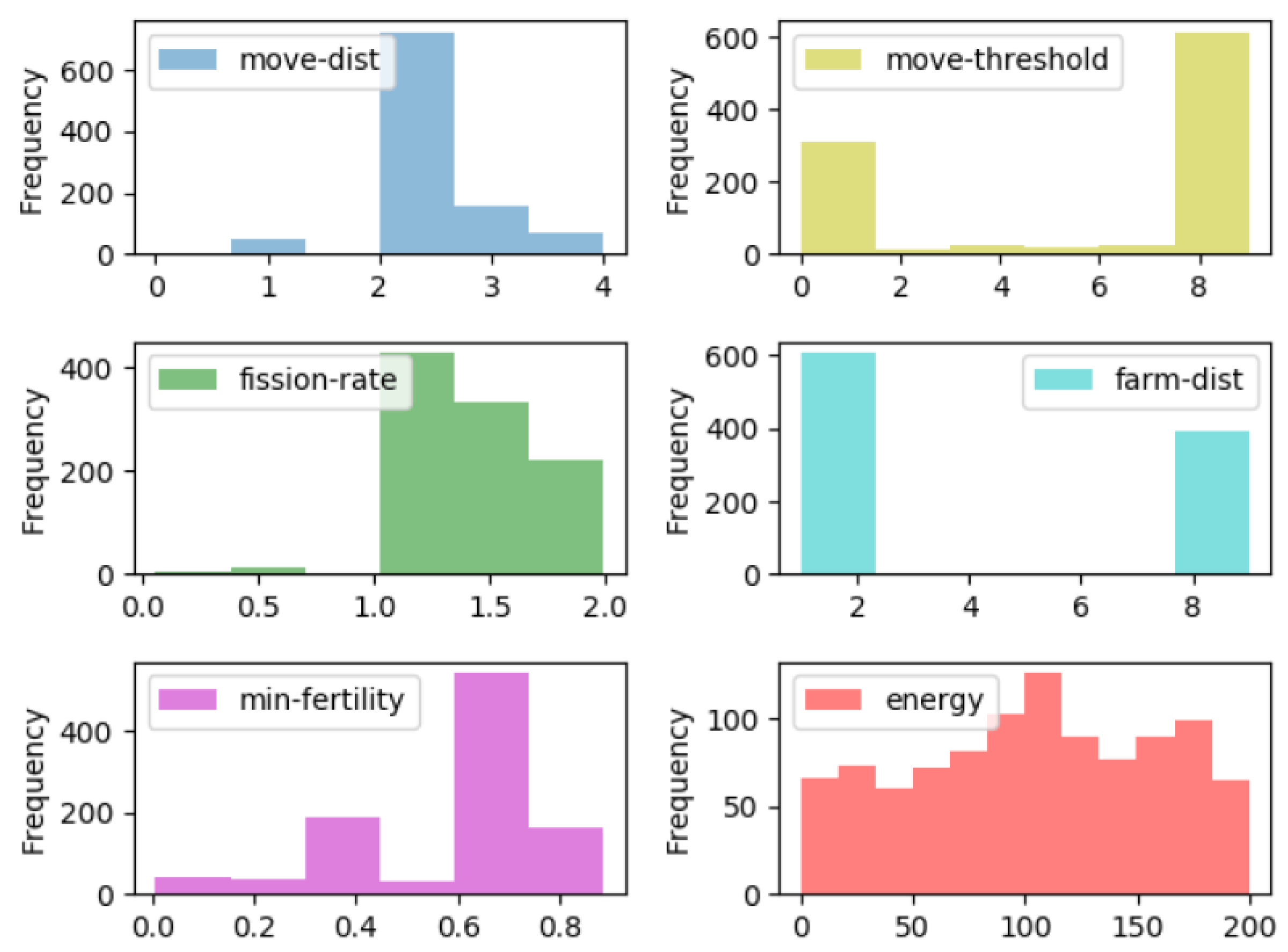
• In turn, simply counting configurations and providing frequencies as done in Figure 10 describes just a small part of the truth, since it completely neglects the actual changes including the differences between two subsequent configurations.
• We can further see that the measurement is independent of changes in the number of participating subsystems, since it just collects samples of configuration vectors no matter how many in a certain time period. This is especially important in the context of open systems, where subsystems are free to join and leave at any time (e.g., in the context of Interwoven System, see [5,60]). However, each new subsystem has a severe impact on the measure.

Besides the pure values received in the scenarios, we can see that the approach fulfils the desired characteristics: it is generic in the sense of being independent of the underlying application scenarios. Completely different parameter configurations are handled in the same way (i.e., as a vector describing a point in the input space) and the computations are just done in a unified way based on the general representation. Consequently, the approach is assumed to be applicable in cases where the system model as outlined in Section 2 is met. The main requirement here is that an external CM needs to alter a parameter vector controlling the behavior of the productive part of a system and that all the parameter vectors of the autonomous subsystems define the configuration space as basis for adaptations.

However, we can already observe some threats to the approach that need to be tackled by future work:

• The values of KL highly depend on the considered feature vector (i.e., the number, the type, and the resolution of the configuration parameters) as well as the frequency in which adaptations are done. These values are highly application-dependent. For a generalized applicability, more studies and a systematic analysis of the search space are required.
• The absolute value of KL cannot be mapped directly to a ’degree of self-adaptation’—it just gives an ordering. It remains subject to future work how this can be done (e.g., by sampling more values of KL and estimating the range of values or synthetically generating strongly deviating distributions based on the specifications of the feature space).
• The changes in the adaptation behavior are quantified as difference between distributions of configurations within measurement cycles. Considering this as novel process or abnormal behavior suggests to augment the approach with mechanisms for anomaly detection (e.g., using approaches for self-adaptive systems as outlined in [61]).
• The considered cases all come with a feasible number of parameters. It remains open how the measurement behaves in high-dimensional spaces (i.e., how the dimensionality problem manifests in this context). However, in such high-dimensional scenarios, the self-adaptation mechanism itself may reach its limits.
• The measure is meant as an approach to analyzing and observing the system behavior at runtime. The determined values will be used as indicators later—which in turn may serve as basis for steering the self-adaptation behavior later (e.g., based on identifying an appropriate level of adaptation).
• The question is still if there can be something like an ’optimal’ degree of self-adaptation. We assume that such a value will not be based on quality attributes only, i.e., those that are already considered in the utility function or in the decision mechanism. In contrast, we user acceptance or stability of the solutions are candidates to consider in such an assessment.

In conclusion, we can state that the proposed measure provides a meaningful indicator for quantification of self-adaptation processes, but it probably needs to be combined with additional information. Other dependency measures replacing $KL$ may be better suitable in the sense of allowing for qualitative statements about the specific values determined by the measure. This is subject to current and future work.

6. Conclusions

This position paper argued that a basic part of an urgently required measurement framework for SASO systems should be dedicated to determining an appropriate degree of self-adaptation. We claimed that on the one hand, too frequent changes will decrease user acceptance, and, on the other hand, more adaptation is key for achieving the underlying system utility. Consequently, one aspect assessing desired SASO behavior is to determine how much adaptation is desirable in which situation. We proposed a concept of how such a measurement can be implemented and defined the required research efforts in terms of four subsequent challenges. Based on two existing simulations, we evaluated and analyzed the behavior of the proposed metric and demonstrated the potential usefulness.

The position paper described a set of challenges for the development of an integrated measurement framework for SASO systems that is based on the initial approach presented here. Our future work is dedicated to closing the outlined research gap. In particular, we will apply the defined method to other scenarios (both other application scenarios as well as artificial models). Furthermore, we will compare the results of the method to other concepts to be developed based on, e.g., clustering techniques or correlation methods. Finally, we will shift the focus towards subsequent measures for, e.g., stability or situation-dependent variability that serves as a basis for self-explanation of SASO behavior.

References

1. Moore, G.E. Cramming more components onto integrated circuits. Electron. Mag. 1965, 38, 114–117. [Google Scholar] [CrossRef]
2. Glass, R.L. Facts and Fallacies of Software Engineering; Agile Software Development, Addison Wesley: Boston, MA, USA, 2002. [Google Scholar]
3. Müller-Schloer, C.; Tomforde, S. Organic Computing—Technical Systems for Survival in the Real World; Springer International Publishing: Cham, Switzerland, 2017. [Google Scholar]
4. Kephart, J.; Chess, D. The Vision of Autonomic Computing. IEEE Comp. 2003, 36, 41–50. [Google Scholar] [CrossRef]
5. Tomforde, S.; Hähner, J.; Sick, B. Interwoven Systems. Informatik-Spektrum 2014, 37, 483–487. [Google Scholar] [CrossRef]
6. Kounev, S.; Lewis, P.; Bellman, K.L.; Bencomo, N.; Camara, J.; Diaconescu, A.; Esterle, L.; Geihs, K.; Giese, H.; Götz, S.; et al. The Notion of Self-aware Computing. In Self-Aware Computing Systems; Springer International Publishing: Cham, Switzerland, 2017; pp. 3–16. [Google Scholar]
7. Shaw, M.; Objects, B. Software design paradigm based on process control. ACM Softw. Eng. Notes 1995, 20, 27–39. [Google Scholar] [CrossRef]
8. Prothmann, H.; Tomforde, S.; Branke, J.; Hähner, J.; Müller-Schloer, C.; Schmeck, H. Organic Traffic Control. In Organic Computing—A Paradigm Shift for Complex Systems; Birkhäuser Verlag: Basel, Switzerland, 2011; pp. 431–446. [Google Scholar]
9. Krupitzer, C.; Roth, F.M.; VanSyckel, S.; Schiele, G.; Becker, C. A survey on engineering approaches for self-adaptive systems. Pervasive Mobile Comput. 2015, 17, 184–206. [Google Scholar] [CrossRef]
10. Rudolph, S.; Tomforde, S.; Sick, B.; Hähner, J. A mutual influence detection algorithm for systems with local performance measurement. In Proceedings of the 2015 IEEE 9th International Conference on Self-Adaptive and Self-Organizing Systems, Cambridge, MA, USA, 21–25 September 2015; pp. 144–149. [Google Scholar]
11. Tomforde, S. From “Normal” to “Abnormal”: A Concept for Determining Expected Self-Adaptation Behaviour. In Proceedings of the 2019 IEEE 4th International Workshops on Foundations and Applications of Self* Systems (FAS*W), Umea, Sweden, 16–20 June 2019; pp. 1–6. [Google Scholar]
12. Tomforde, S.; Prothmann, H.; Branke, J.; Hähner, J.; Mnif, M.; Müller-Schloer, C.; Richter, U.; Schmeck, H. Observation and Control of Organic Systems. In Organic Computing—A Paradigm Shift for Complex Systems; Birkhäuser: Basel, Switzerland, 2011; pp. 325–338. [Google Scholar]
13. Kantert, J.; Edenhofer, S.; Tomforde, S.; Hähner, J.; Müller-Schloer, C. Normative Control—Controlling Open Distributed Systems with Autonomous Entities. In Trustworthy Open Self-Organising Systems; Birkäuser: Basel, Switzerland, 2016; pp. 89–126. [Google Scholar]
14. Chan, W. Interaction Metric of Emergent Behaviours in Agent Simulations. In Proceedings of the 2011 Winter Simulation Conference (WSC), Phoenix, AZ, USA, 11–14 December 2011; pp. 357–368. [Google Scholar]
15. Eberhardinger, B.; Anders, G.; Seebach, H.; Siefert, F.; Reif, W. A research overview and evaluation of performance metrics for self-organization algorithms. In Proceedings of the Self-Adaptive and Self-Organizing Systems Works (SASO-W’15), Cambridge, MA, USA, 21–25 September 2015; pp. 122–127. [Google Scholar]
16. Kaddoum, E.; Raibulet, C.; Georgé, J.P.; Picard, G.; Gleizes, M.P. Criteria for the Evaluation of Self-* Systems. In Proceedings of the ICSE Workshop on Software Engineering for Adaptive and Self-Managing Systems, Cape Town, South Africa, 3–4 May 2010; pp. 29–38. [Google Scholar]
17. Cámara, J.; Correia, P.; de Lemos, R.; Vieira, M. Empirical resilience evaluation of an architecture-based self-adaptive software system. In Proceedings of the ACM Sigsoft Conference on Quality of Software Architectures, Lille, France, 30 June– 4 July 2014; pp. 63–72. [Google Scholar]
18. Gronau, N. Determinants of an Appropriate Degree of Autonomy in a Cyber-physical Production System. Procedia CIRP 2016, 52, 1–5. [Google Scholar] [CrossRef] [Green Version]
19. Brown, D.; Goodrich, M. Limited bandwidth recognition of collective behaviours in bio-inspired swarms. In Proceedings of the International Conference on Autonomous Agents and Multi-Agent Systems, Paris, France, 5–9 May 2014; pp. 405–412. [Google Scholar]
20. O’Toole, E.; Nallur, V.; Clarke, S. Towards Decentralised Detection of Emergence in Complex Adaptive Systems. In Proceedings of the of IEEE International Conference on Self-Adaptive and Self-Organizing Systems (SASO’14), London, UK, 8–12 September 2014; pp. 60–69. [Google Scholar]
21. Deaton, J.; Allen, R. Development and application of system complexity measures for use in modeling and simulation. In Proceedings of the Conference on Summer Computer Simulation, Chicago, IL, USA, 26–29 July 2015; pp. 1–6. [Google Scholar]
22. Shalizi, C.R.; Shalizi, K.L. Quantifying Self-Organization in Cyclic Cellular Automata. In Proceedings of the SPIE Noise in Complex Systems and Stochastic Dynamics, Bellingham, WA, USA, 7 May 2003; pp. 108–117. [Google Scholar]
23. Heylighen, F. The Science of Self-Organization and Adaptivity. In Knowledge Management, Organizational Intelligence and Learning, and Complexity; Encyclopedia of Life Support Systems: Oxford, UK, 1999; pp. 253–280. [Google Scholar]
24. Wright, W.; Smith, R.E.; Danek, M.; Greenway, P. A Generalisable Measure of Self-Organisation and Emergence. In Proceedings of the International Conference on Artificial Neural Networks (ICANN’01), Vienna, Austria, 21–25 August 2001; Springer: Cham, Switzerland, 2001; pp. 857–864. [Google Scholar]
25. Gershenson, C.; Fernandez, N. Complexity and Information: Measuring Emergence, Self-organization, and Homeostasis at Multiple Scales. Complexity 2012, 18, 29–44. [Google Scholar] [CrossRef] [Green Version]
26. Schmeck, H.; Müller-Schloer, C.; Çakar, E.; Mnif, M.; Richter, U. Adaptivity and Self-organization in Organic Computing Systems. ACM Trans. Auton. Adapt. Syst. 2010, 5, 1–32. [Google Scholar] [CrossRef]
27. Kantert, J.; Tomforde, S.; Müller-Schloer, C. Measuring Self-Organisation in Distributed Systems by External Observation. In Proceedings of the 28th GI/ITG International Conference on Architecture of Computing Systems—ARCS Workshop on Self-Optimisation in Organic and Autonomic Computing Systems (SAOS15), Porto, Portugal, 24–27 March 2015; pp. 1–8. [Google Scholar]
28. Rudolph, S.; Kantert, J.; Jänen, U.; Tomforde, S.; Hähner, J.; Müller-Schloer, C. Measuring Self-Organisation Processes in Smart Camera Networks. In Proceedings of the 29th International Conference on Architecture of Computing Systems (ARCS 2016); Varbanescu, A.L., Ed.; VDE Verlag GmbH: Nuremberg, Germany, 2016; Chapter 14; pp. 1–6. [Google Scholar]
29. Tomforde, S.; Kantert, J.; Sick, B. Measuring Self-organisation at Runtime—A Quantification Method Based on Divergence Measures. In Proceedings of the 9th International Conference on Agents and Artificial Intelligence (ICAART 2017), Porto, Portugal, 24–26 February 2017; Volume 1, pp. 96–106. [Google Scholar]
30. Filieri, A.; Maggio, M.; Angelopoulos, K.; D’ippolito, N.; Gerostathopoulos, I.; Hempel, A.B.; Hoffmann, H.; Jamshidi, P.; Kalyvianaki, E.; Klein, C.; et al. Control Strategies for Self-Adaptive Software Systems. ACM Trans. Auton. Adapt. Syst. 2017, 11, 24:1–24:31. [Google Scholar] [CrossRef] [Green Version]
31. Shalizi, C.R. Causal Architecture, Complexity and Self-Organization in the Time Series and Cellular Automata. Ph.D. Thesis, University of Wisconsin–Madison, Madison, WI, USA, 2001. [Google Scholar]
32. Prokopenko, M.; Boschetti, F.; Ryan, A.J. An information-theoretic primer on complexity, self-organisation and emergence. Complexity 2007, 15, 11–28. [Google Scholar] [CrossRef]
33. Holzer, R.; de Meer, H. Methods for Approximations of Quantitative Measures in Self-Organizing Systems. In Proceedings of the 5th International Works on Self-Organizing Systems (IWSOS’11), Karlsruhe, Germany, 23–24 February 2011; pp. 1–15. [Google Scholar]
34. Mnif, M.; Müller-Schloer, C. Quantitative emergence. In Organic Computing—A Paradigm Shift for Complex Systems; Springer: Cham, Switzerland, 2011; pp. 39–52. [Google Scholar]
35. Fisch, D.; Janicke, M.; Sick, B.; Muller-Schloer, C. Quantitative Emergence—A Refined Approach Based on Divergence Measures. In Proceedings of the 2010 Fourth IEEE International Conference on Self-Adaptive and Self-Organizing Systems, Budapest, Hungary, 27 September–1 October 2010; pp. 94–103. [Google Scholar]
36. Chen, T.; Bahsoon, R.; Wang, S.; Yao, X. To adapt or not to adapt? Technical debt and learning driven self-adaptation for managing runtime performance. In Proceedings of the 2018 ACM/SPEC International Conference on Performance Engineering, Berlin, Germany, 9–13 April 2018; pp. 48–55. [Google Scholar]
37. Bishop, C. Pattern Recognition and Machine Learning, 2nd ed.; Information Science and Statistics; Springer: Cham, Switzerland, 2011. [Google Scholar]
38. Tomforde, S.; Kantert, J.; Müller-Schloer, C.; Bödelt, S.; Sick, B. Comparing the Effects of Disturbances in Self-adaptive Systems—A Generalised Approach for the Quantification of Robustness. Trans. Comput. Collect. Intell. 2018, 28, 193–220. [Google Scholar]
39. Rudolph, S.; Tomforde, S.; Hähner, J. A Mutual Influence-based Learning Algorithm. In Proceedings of the International Conference on Agents and Artificial Intelligence (ICAART16), Porto, Portugal, 24–26 February 2016; pp. 181–189. [Google Scholar]
40. Rudolph, S.; Tomforde, S.; Hähner, J. Mutual Influence-aware Runtime Learning of Self-adaptation Behavior. TAAS 2019, 14, 4:1–4:37. [Google Scholar] [CrossRef]
41. Prothmann, H.; Branke, J.; Schmeck, H.; Tomforde, S.; Rochner, F.; Hähner, J.; Müller-Schloer, C. Organic traffic light control for urban road networks. IJAACS 2009, 2, 203–225. [Google Scholar] [CrossRef]
42. Prothmann, H.; Rochner, F.; Tomforde, S.; Branke, J.; Müller-Schloer, C.; Schmeck, H. Organic Control of Traffic Lights. In Proceedings of the 5th International Conference on Autonomic and Trusted Computing (ATC-08), Oslo, Norway, 23–25 June 2008; Rong, C., Ed.; Springer: Cham, Switzerland, 2008; Volume 5060, pp. 219–233. [Google Scholar]
43. Tomforde, S.; Prothmann, H.; Rochner, F.; Branke, J.; Hähner, J.; Müller-Schloer, C.; Schmeck, H. Decentralised Progressive Signal Systems for Organic Traffic Control. In Proceedings of the 2nd IEEE International Conference on Self-Adaption and Self-Organization (SASO’08), Venice, Italy, 20–24 October 2008; pp. 413–422. [Google Scholar]
44. Sommer, M.; Tomforde, S.; Hähner, J. An Organic Computing Approach to Resilient Traffic Management. In Autonomic Road Transport Support Systems, Autonomic Systems ed.; McCluskey, T.L., Kotsialos, A., Müller, J.P., Klügl, F., Rana, O., Schumann, R., Eds.; Birkhäuser Verlag: Basel, Switzerland, 2016; pp. 113–130. [Google Scholar]
45. Barceló, J.; Casas, J. Dynamic network simulation with AIMSUN. In Simulation Approaches in Transportation Analysis; Springer: Cham, Switzerland, 2005; pp. 57–98. [Google Scholar]
46. Gabbard, J. Car-Following Models, Concise Encyclopedia of Traffic and Transportation Systems; Papageorgiou, M., Ed.; Pergamon Press: Oxford, UK, 1991. [Google Scholar]
47. Barton, C.M. Complexity, social complexity, and modeling. J. Archaeol. Method Theory 2014, 21, 306–324. [Google Scholar] [CrossRef]
48. Wilensky, U.; Rand, W. An Introduction to Agent-Based Modeling: Modeling Natural, Social, and Engineered Complex Systems with NetLogo; MIT Press: Cambridge, MA, USA, 2015. [Google Scholar]
49. Tomforde, S.; Cakar, E.; Hähner, J. Dynamic Control of Network Protocols—A new vision for future self-organised networks. In Proceedings of the 6th International Conference on Informatics in Control, Automation, and Robotics (ICINCO’09), Milan, Italy, 2–5 July 2009; Filipe, J., Cetto, J.A., Ferrier, J.L., Eds.; INSTICC: Milan, Italy, 2009; pp. 285–290. [Google Scholar]
50. Tomforde, S.; Steffen, M.; Hähner, J.; Müller-Schloer, C. Towards an Organic Network Control System. In Proceedings of the 6th International Conference on Autonomic and Trusted Computing (ATC’09), Brisbane, Australia, 7–10 July 2009; Springer: Cham, Switzerland, 2009; pp. 2–16. [Google Scholar]
51. Tomforde, S.; Hurling, B.; Hähner, J. Distributed Network Protocol Parameter Adaptation in Mobile Ad-Hoc Networks. In Informatics in Control, Automation and Robotics; Springer: Berlin/Heidelberg, Germany, 2011; Volume 89, pp. 91–104. [Google Scholar]
52. Tomforde, S.; Hurling, B.; Hähner, J. Adapting parameters of mobile ad-hoc network protocols to changing environments. In Informatics in Control, Automation and Robotics—Selected Papers from the International Conference on Informatics in Control, Automation and Robotics 2010; Andrade-Cetto, J., Ferrier, J.L., Filipe, J., Eds.; Lecture Notes in Electrical Engineering Series Number 81; Springer: Berlin/Heidelberg, Germany, 2011; pp. 91–104. [Google Scholar]
53. Tomforde, S.; Ostrovsky, A.; Hähner, J. Load-Aware Reconfiguration of LTE Antennas—Dynamic Cell-Phone Network Adapta-tion Using Organic Network Control. In Proceedings of the 11th International Conference on Informatics in Control, Automation, and Robotics (ICINCO’14), Vienna, Austria, 2–4 September 2014; pp. 243–263. [Google Scholar]
54. Hähner, J.; Streit, K.; Tomforde, S. Cellular traffic offloading through network-assisted ad-hoc routing in cellular networks. In Proceedings of the 2016 IEEE Symposium on Computers and Communication (ISCC), Messina, Italy, 27–30 June 2016; pp. 469–476. [Google Scholar]
55. Tomforde, S.; Gruhl, C.; Haehner, J. A Concept for Self-adapting and Self-learning Traffic Offloading in Cellular Networks. In Proceedings of the 30th International Conference on Architecture of Computing Systems (ARCS 2017), Vienna, Austria, 4–6 April 2017; pp. 1–8. [Google Scholar]
56. Tomforde, S.; Kantert, J.; von Mammen, S.; Hähner, J. Cooperative Self-Optimisation of Network Protocol Parameters at Runtime. In Proceedings of the ICINCO’15, Madeira, Portugal, 21–23 July 2015; pp. 123–130. [Google Scholar]
57. Kunz, T. Reliable Multicasting in MANETs. Ph.D. Thesis, Carleton University, Ottawa, ON, Canada, 2003. [Google Scholar]
58. Luke, S.; Cioffi-Revilla, C.; Panait, L.; Sullivan, K. MASON: A New Multi-Agent Simulation Toolkit. In Proceedings of the 2004 Swarmfest Workshop, Budapest, Hungary, 10–15 May 2004. [Google Scholar]
59. Fall, K. Network Emulation in the Vint/NS Simulator. In Proceedings of the 4th IEEE Symposium on Computers and Communications (ISCC’99), Red Sea, Egypt, 6–8 July 1999; p. 244. [Google Scholar]
60. Bellman, K.L.; Gruhl, C.; Landauer, C.; Tomforde, S. Self-Improving System Integration—On a Definition and Characteristics of the Challenge. In Proceedings of the IEEE 4th International Workshops on Foundations and Applications of Self* Systems (FAS*W@SASO/ICCAC 2019), Umea, Sweden, 16–20 June 2019; pp. 1–3. [Google Scholar]
61. Gruhl, C.; Sick, B.; Wacker, A.; Tomforde, S.; Hähner, J. A building block for awareness in technical systems: Online novelty detection and reaction with an application in intrusion detection. In Proceedings of the 2015 IEEE 7th International Conference on Awareness Science and Technology (iCAST), Qinhuangdao, China, 22–24 September 2015; pp. 194–200. [Google Scholar]
Figure 1. Schematic illustration of a subsystem a i . Green arrows indicate observation flows, while red arrows indicate control flows. Dashed arrows emphasize a possible path that is typically not used.
Computers 09 00021 g001
Figure 2. Estimating the stability of system adaptation after disturbances.
Computers 09 00021 g002
Figure 3. Example of a four-armed intersection.
Computers 09 00021 g003
Figure 4. Definition of phases for the individual traffic lights as a basis for the setup of the signal plan.
Computers 09 00021 g004
Figure 5. Setup of an example signal plan for the intersection of Figure 3.
Computers 09 00021 g005
Figure 6. Simulated Stadium Area at Hannover, Germany.
Computers 09 00021 g006
Figure 7. Averaged delays in the simulation for the reference solution and the OTC controlled simulation.
Computers 09 00021 g007
Figure 8. Screenshot of the simulation: Dark green background is uncleared woodland (not assigned to a household), lighter green circles are areas of uncleared woodland assigned to households, farmsteads are indicated by red house icons in the center of the lighter green circles, brown patches are currently farmed; white through light green patches represent regrowing vegetation.
Computers 09 00021 g008
Figure 9. Number of agents over the simulation period of 1000 steps.
Computers 09 00021 g009
Figure 10. Analysis of the occurrences of configurations per parameter.
Computers 09 00021 g010