Abstract
Modern Monte-Carlo-based rendering systems still suffer from the computational complexity involved in the generation of noise-free images, making it challenging to synthesize interactive previews. We present a framework suited for rendering such previews of static scenes using a caching technique that builds upon a linkless octree. Our approach allows for memory-efficient storage and constant-time lookup to cache diffuse illumination at multiple hitpoints along the traced paths. Non-diffuse surfaces are dealt with in a hybrid way in order to reconstruct view-dependent illumination while maintaining interactive frame rates. By evaluating the visual fidelity against ground truth sequences and by benchmarking, we show that our approach compares well to low-noise path-traced results, but with a greatly reduced computational complexity, allowing for interactive frame rates. This way, our caching technique provides a useful tool for global illumination previews and multi-view rendering.
1. Introduction
This article is an extension to our publication at the 37th Computer Graphics & Visual Computing Gathering 2019 [1].
Global illumination (GI) rendering based on Monte Carlo (MC) methods allows for the generation images of astonishing realism that can often hardly be distinguished from real photographs. Even though these methods have been around for a long time, their computational complexity remains a major challenge. Ray-based approaches like path tracing may require a considerable number of rays to be traced through a scene to determine an approximate solution for the Rendering Equation [2]. Because of the stochastic nature of this process, this can take anywhere from mere seconds to hours until a noise-free result emerges. While the realism gained by accounting for GI is often considerable, rendering previews in current 3D modeling software often does not result in images with the same fidelity due to the limited processing time and the usage of different rendering methods. In recent years, numerous methods have been introduced that help to increase the visual quality by filtering the noise from images rendered with low sample counts. These methods often result in visually pleasing, noise-free images. However, rendering the GI of a scene usually involves computing the light transport at a large number of points that are not directly visible in image space. When moving through the scene, reusing this information for the computation of successive frames can increase visual quality and shorten rendering times at the same time.
We introduce the HashCache, a hierarchical world-space caching method for GI rendering of static scenes, based on a linkless octree [3]. Using a hash-based approach makes it possible to perform the reconstruction of cached illumination in constant time, depending only on the actual screen resolution (assuming that the visible geometry is known). This makes it well-suited for the exploration of static scenes. Despite only caching diffuse illumination, our system explicitly supports non-diffuse materials through a hybrid reconstruction scheme. This is an approximate final gathering step similar to Photon Mapping [4,5] and is performed before the actual reconstruction. For non-diffuse materials, this step is composed in a hybrid way: Rays are traced up to the first hitpoint that is interpreted as a diffuse material, where the pre-gathered information is then queried from the cache and modulated with the path throughput. This process is described in more detail in Section 3.2, Section 3.3 and Section 3.4. Compared to precomputed radiance transfer, our preprocessing time is much shorter, as we only need to determine geometric cell occupations.
In order to reduce quantization artifacts, we employ a spatial jittering method inspired by Binder et al. [6]. To increase image quality by reducing noise, we suggest a layered filtering framework, basically projecting path-space filtering [7] to image space. In order to demonstrate the practicability of our approach, we extend a basic cross-bilateral denoising filter by integrating it into our framework and adjusting it to the kind of noise present in our system, enabling it to filter the image content per light bounce. With this method, we especially aim for improving the visual quality of non-diffuse materials, compared to filtering only at the primary hitpoint without any information about the transport paths. Arbitrary image-space filtering methods may be integrated into the suggested framework in order to improve their handling of specular or glossy material types. Finally, we present image quality comparisons, performance benchmarks, and an analysis of memory requirements, showing the practicability of our approach. While maintaining interactive frame rates, the noise in the image can be reduced significantly. We show that our approach performs comparably to much higher sampling rates in path tracing regarding relative mean square error (relMSE) and multi-scale structural similarity (MS-SSIM) metrics.
2. Related Work
Caching samples is a proven tool for several computer graphics applications. An overview of some of the relevant work from this area has been published by Scherzer et al. [8]. Currently, most methods try to exploit the temporal coherence in image space. However, caching in world space has the advantage of prolonging the validity of samples in the cases of view-dependent (dis-)occlusions and surfaces that are not directly visible. This is especially beneficial for methods that handle indirect GI. In addition to caching methods, filtering techniques have been introduced to allow for real-time rendering with low sampling rates while maintaining acceptable image quality. In the following section, we elaborate on an overview of the relevant research related to our system, including the fields of sample caching, interactive GI, and filtering, as we combine methods from these fields.
Early work by Ward et al. [9] uses an octree to cache irradiance values in world space. This approach is easy to implement when rays are cast sequentially. However, updating a data structure is challenging when data are accessed in a parallel fashion. Bala et al. [10] already presented a ray tracer suited for near-interactive scene editing in 1999. Their visualization is based on object-space radiance interpolation and a hierarchical data structure called ray segment trees. The latter is introduced for tracking the dependencies between radiance interpolations for regions in world space, and helps with illumination updates triggered by scene manipulations. The Render Cache by Walter et al. [11] is an interactive caching and reprojection technique with adaptive sampling. In order to be efficient, only samples within the view frustum are reprojected from one frame to the next. GI computations on surfaces outside the current frame’s frustum are not cached at all. Ward and Simmons [12] already worked on nondiffuse interactive global illumination in the same year, introducing their holodeck ray cache. The eponymous holodeck is a four-dimensional data structure that provides a caching mechanism for interactive walk-throughs. Sample density is varied locally, while sampling happens on-demand and is implemented in a parallel fashion. While allowing for dynamically illuminated environments, the precomputed radiance transfer system for real-time rendering presented by Sloan et al. [13] only supports low-frequency content. Spherical harmonics are used for representing illumination information for glossy and diffuse materials alike. In addition, a method is suggested for rendering soft shadows and caustics from rigidly moving objects onto dynamic receivers. Tole et al. [14] introduced a caching scheme that supports the interactive computation of global illumination in dynamic scenes. Their Shading Cache is an object-space hierarchical subdivision mesh that stores shading values at its vertices. Hardware-based interpolation and texture mapping make it possible to generate results at high frame rates, while the results are adaptively refined based on the interpolation error and camera or object motion. Images with a suitable quality are generated within tens of seconds, outperforming other systems that were available at the time.
The interactive rendering and display technique suggested by Bala et al. [15] supports complex scenes with complex shading such as global illumination. Sparsely distributed samples and analytically computed edges are combined in a way that allows for generating images of a relatively high quality by relying on a compact edge-and-point image. The presented renderer supports scene interaction such as object manipulation and achieved a performance of 8 to 14 frames per second on a desktop PC at the time. The findings of Krivànek et al. [16] are based on Ward et al.’s earlier work [9]. The authors present a method for efficient global illumination that relies on sparse sampling, caching, and interpolation. More specifically, the older irradiance caching scheme is extended so that radiance, instead of irradiance, can be cached and interpolated. In work by Christensen et al. [17], a sparse octree is suggested as a 3D Mipmap to store irradiance values. A brick structure is employed to store sparse samples for individual octree cells. Dietrich et al. [18] propose a cache that employs a hash map as the spatial index structure to store shading and illumination without the need for a preprocessing step. While our presented work shares many similarities with this approach, the hashing mechanism by Dietrich et al. cannot be easily ported to highly parallel systems such as the GPU. Moreover, they provide neither a level-of-detail mechanism nor a method to filter the results. A method for temporal radiance caching that supports glossy global illumination in animated environments is presented by Gautron et al. [19]. Their approach is built upon irradiance and radiance caching, while sparse temporal sampling and interpolation of indirect lighting are employed to reuse the computed information in succeeding frames. Lighting information is adaptively updated and flickering artifacts are strongly reduced. Their temporal interpolation approach is based on temporal gradients. According to the authors, one of the key advantages of their method is the straightforward implementation into any existing renderer. Brouillat et al. [20] introduce the combination of photon mapping and irradiance caching. More specifically, their approach computes an irradiance cache from a photon map. This means that the advantage of photon mapping being view-independent is exploited to perform view-independent irradiance caching, while the actual rendering is done using radiance cache splatting. Radiance Caching by Krivànek et al. [21] is a method for accelerating GI computation in scenes with low-frequency glossy bidirectional reflectance distribution functions (BRDFs) based on spherical harmonics. Higher-frequency content is supported in work by Omidvar et al. [22], using Equivalent Area Light Sources. However, all of the methods presented so far are offline processes for non-interactive systems.
Multi-bounce indirect lighting, glossy reflections, arbitrary specular paths, and thus even caustics are supported in Wang et al.’s work [23], which builds upon scattered data interpolation on the GPU. Interpolation is supported by k-mean clustering and a subsequent final gathering step, where the photon map is approximated using lightcuts. Using this method, it is possible for the user to manipulate the viewed scene at interactive frame rates. Hachisuka and Jensen [24] describe how to use spatial hashing for constructing photon maps on the GPU. Their method stores a single photon stochastically instead of storing lists or aggregations. This allows the approach to ignore hash collisions but limits the sample set size and expressiveness. Caching samples in world space is either computationally demanding or only worked for a limited set of samples because of memory requirements. Hence, there is a need for fast world-space sample-caching techniques that allow updating aggregated samples. Keeping GPU implementations in mind, it is crucial for these updates to be suited for parallel execution.
Crassin et al. [25] provide a technique for real-time GI based on approximate cone tracing using a sparse voxel octree. However, the appearance differs between renderings generated with their method and unbiased results. A real-time approach for approximating GI is presented by Thiedemann et al. [26]. While diffuse near-field GI is rendered at high visual fidelity, voxel-based visibility computation causes glossy reflections not to be handled well.
Ritschel et al. [27] present a comprehensive summary of the major challenges in interactive GI. Their work includes the underlying theoretical aspects, phenomena, and methods for the actual rendering task. They also provide an overview of ratings regarding various aspects like ease of implementation, also giving information about the transport paths that each method can handle. The radiance-caching method proposed by Scherzer et al. [28] uses pre-filtered cache items based on MIP-maps as a substitute for spherical harmonics. The coefficient-dependent complexity of spherical harmonics is thus replaced by a constant-time lookup per pixel, improving performance by an order of magnitude when compared to radiance caching with Phong BRDFs. Fast approximations of joint bilateral filtering (as presented by Dammertz et al. [29] and Bauszat et al. [30]) and utilizing adaptive manifolds [31] also help with increasing the image quality and reducing noise. Mara et al. [32] present a method for efficient density estimation for photon mapping on the GPU. While their work also contains information on using a hash map as their data structure, it is strictly limited to photon mapping. Our approach, however, can be used with several GI methods. An overview of filtering techniques for preview rendering is given by Schwenk [33]. Intuitively editing the appearance in complex scenes (geometry- and lighting-wise alike) poses a major challenge. Nguyen et al. [34] present a method that enables the user to freely manipulate surface light fields. Surface reflectance functions are then adapted to best fit the desired surface light field by changing shading parameters. In contrast to earlier approaches, manipulating the surface light field is possible by using a single color brush tool.
Our layered filtering approach is inspired by Keller et al.’s path-space filtering [7]. Here, the contribution of actual light transport paths is smoothed before reconstruction. While this method performs a range search in path space, our approach effectively brings this filtering to screen-space in a way that is simple to implement. The general decomposition method for filtering specific light paths presented by Zimmer et al. [35] is closely related to our approach. However, the decomposition in our algorithm is exclusively based on recursion depth, not directly taking specific material properties into account. This results in an easier, more straightforward implementation.
Munkberg et al. [36] present a method for caching illumination in texture space. While their approach avoids the issues of axis-aligned grids and strongly supports the use of material-specific filters, a global approach like ours makes it easier to account for arbitrary neighboring geometry in the filtering process. Chaitanya et al. [37] present a technique for reconstructing image sequences based on autoencoders, motivated by recent advances in image restoration with deep convolutional networks. Another method from the same field is presented by Bako et al. [38], with the focus put on high-end, production-quality renderings. The authors also provide a comparison of these two related approaches. A direct-to-indirect transport technique is described by Silvennoinen et al. [39]. It is suited for mostly static scenes with fully dynamic lighting, cameras, and diffuse materials, with the incident radiance field being reconstructed from a sparse set of radiance probes. Global illumination is then computed by factorizing the direct-to-indirect transport into two parts—global and local—sampling the global transport with the aforementioned radiance probes and using the sampled radiance field for a reconstruction filter. While the achieved visual quality is convincing, this method requires a relatively long precomputation time of around one hour for the presented scenes. Our method works magnitudes faster to preprocess the scene’s geometry and to build the hashing structure.
Schied et al. [40,41] suggest methods for generating temporally stable image sequences from GI at one sample per pixel. The effective sample count available to their approach is increased by accumulating samples temporally, while the denoising method itself is performed by using a hierarchical image-space wavelet filter. Note that Binder et al. [6] also mention a way of filtering similar to ours as a possible future solution to overcome artifacts. The main contribution of their work is a fast path-space filtering method by using jittered spatial hashing for hiding quantization artifacts. While Binder et al. do not use caching, they also utilize a hash-based approach in order to optimize neighborhood search. Their jittering method is also applicable in our case for hiding quantization artifacts introduced by the discrete scene subdivision.
Binder et al. [42] provide a massively parallel GPU implementation of path-space filtering using a hash table for searching nearby vertices. This is related to our layered filtering approach, as filtering for both does not only happen on the primary hitpoints, but vertices of paths are shared between pixels when filtering the image. In contrast to approaches like Binder et al.’s, our method projects the information available in path space to the according pixels in screen space, but puts the information from subsequent vertices to different layers, which are then filtered individually. Real-time glossy and specular reflections are improved by combining ray tracing with radiance probes and screen-space reflections in Hirvonen et al.’s work [43], while Luksch et al. [44] propose a system for incrementally updating baked global illumination solutions in order to avoid visual disturbances such as flickering or noise. Their many-light GI algorithm is combined with appropriate data structures and prioritization strategies in order to compute differential updates for illumination states. Wang et al. [45] provide some novel work regarding light-field probes. Their non-uniform placement method has the goal of correctly sampling visibility information and eliminating superfluous probes at the same time. Probe placement relies on scene skeletons and a refinement based on gradient descent. Visibility is cached in a sparse voxel octree. Yalçıner and Sahillioğlu [46] present a method for populating sparse voxel octrees in the presence of a high number of dynamic objects. Their pre-generated voxel data are transformed from model space to world space on demand, while common approaches voxelize dynamic objects per frame. An additional filtering method enables smooth transitions and reduces aliasing. The authors provide a real-world use case by implementing voxel cone tracing with their discretization method. Zhao et al. [47] introduce an approach for improving the reconstruction of glossy interreflections, while also showing performance gains when compared to previous approaches. Their view-dependent radiance caching works directly with outgoing radiance at surfaces instead of incoming radiance distributions. In a recent paper, Huo et al. [48] propose the use of quality and reconstruction networks with a large offline dataset for the adaptive sampling and reconstruction of first-bounce incident radiance fields. The reconstruction network is based on a convolutional neural network. Reconstruction happens in 4D space. At the same time, the quality network is based on deep reinforcement learning and guides the adaptive sampling process. Comparisons with state-of-the-art methods show visually convincing results.
All of the methods above greatly benefit from exploiting spatial and/or temporal coherence in image space. We argue that a world-space sample-caching technique can further improve the image quality of such filtering methods, especially in complex scenes with many occluding surfaces and arbitrary views.
3. Method
In this section, we give an overview of the employed cache structure and describe how it can be used to cache the data generated by stochastic rendering methods. Subsequently, we give more details on how samples are generated during the rendering process in order to reuse recursively generated hitpoints. Here, it is also shown how the actual cache updates are performed. Eventually, we provide information about the reconstruction process, including the support of non-diffuse materials, as well as our proposed layered filtering framework.
3.1. Cache Structure
Monte-Carlo-based (MC-based) rendering methods provide the means to solve Kajiya’s Rendering Equation [2] numerically. In our implementation, a straightforward path tracer with next-event estimation and multiple-importance sampling is used for computing the illumination data. The path-tracing process generates millions of randomly and sparsely distributed hitpoints located on the scene geometry in each iteration, which means that we are not supporting participating media to be cached. Consequently, a data structure that allows for efficient caching of such data must allow for querying of large amounts of randomly distributed keys at a high performance. The core of our HashCache system is Choi et al.’s concept of a linkless octree [3], consisting of a number of hash maps implemented with Alcantara’s Cuckoo Hashing [49]. This hashing method allows for a worst-case constant lookup time, making its choice especially suitable for real-time previews. Cuckoo hashing resolves collisions by employing an additional hash function in order to compute two candidate indices in the hash table for one key. When a collision is detected on key insertion, the already-existing entry is replaced by the new entry. Then, the old entry is inserted at its alternative position, with potential collisions handled the same way iteratively until all entries have been successfully placed. While the result may be an infinite loop, this issue can be detected and the process can then be restarted with alternative hash functions. Although it was possible to use a plain grid instead of an octree, we chose to use the hierarchical approach for its inherent level-of-detail support. When rendering a scene from an arbitrary point of view using a non-hierarchical data structure, parts of this data structure will be potentially subsampled, resulting in aliasing artifacts. With a hierarchical data structure like the HashCache, it is possible to choose the hierarchy’s level whose resolution most closely resembles the projected pixel size in object space, hiding subsampling artifacts effectively.
While the hash-based octree representation is a compact structure, there still is a trade-off between memory consumption and access time. In order to construct the compact hash map, all cells occupied with geometry have to be marked at the highest resolution available in the octree. This information is determined by testing all grid cells within each triangle’s bounding box for an intersection with the triangle, resembling typical grid construction algorithms, such as in the work by Perard-Gayot et al. [50]. Because of the large number of grid cells at high resolutions, we choose to represent each cell by a single bit in a field of 32 bit types. Each 32 bit chunk forms a block, which is subdivided spatially at a resolution of bits = 32 bits. The implementation uses CUDA’s atomic operations on the respective chunks, effectively yielding the number of occupied cells. For an illustration of our approach for determining occupied cells, see Figure 1 and Figure 2.
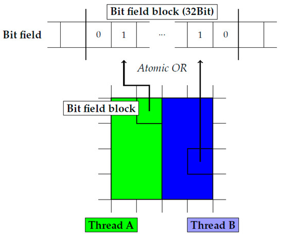
Figure 1.
Marking valid cells in a bit field by 3D rasterization of the grid cells.
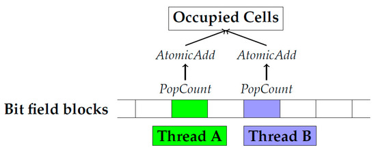
Figure 2.
Computing the total number of the occupied cells using a pop count and an atomic add operation.
During the hash map initialization, this number is used in combination with a space-usage factor to limit the actual memory requirements. We choose an initial space-usage factor of . If the hash map construction fails, another attempt is made with until construction succeeds. This construction process is performed for each octree level, with cell indices being adapted accordingly. As the utilized hash map implementation is bound to 32 bit keys and an octree’s extents are limited to powers of two, the maximum representable resolution is . Higher resolutions are represented by splitting space into multiple hash maps per octree level.
The values stored in the octree’s underlying hash maps are actual indices to global data arrays. These arrays occupy exactly the space required to store all of the information that is computed throughout the process. Note that the presented implementation relies on caching only the outgoing diffuse illumination without any directional information other than the front and back of each cache cell, where the front is determined to be the inverse orientation of the first ray that hits any geometry within a cell. While it would be possible to store information for more directions, this would negatively influence storage requirements and performance. However, storing at least two directions is necessary, since infinitesimally thin geometric primitives may be illuminated differently from both sides. To store more accurate GI information for those cases, we construct the arrays to contain the following data per cell:
- Diffuse illumination for the front and back of each cell as six half values (96 bits);
- compressed cell normal (32 bits);
- currently accumulated number of samples (32 bits);
- the frame index denoting when the cell has last been wiped (32 bits).
Thus, the total amount of memory required for the data of one cell is (12 + 4 + 4 + 4) Bytes = 24 Bytes. The reset information is required to rebuild the cache when illumination changes occur. Note that the diffuse illumination is not attenuated by the diffuse material color (albedo) at this point. Instead, this is accounted for during reconstruction, which allows for a higher-quality representation of spatial variation in the appearance of diffuse surfaces. In order to determine the front normal of each cell, which is required to discern the stored orientations of each cache cell, an atomic compare-and-swap is used to store the current normal in a cache cell if no normal is stored so far. All generated samples can then be assigned to the front or back by comparing their stored normals with the front normal.
There are no specific constraints for the number of triangles per octree cell (or, vice versa, the number of octree cells per triangle), as the required resolution largely depends on the lighting situation and the actual camera settings and position—for quick previews during modeling of individual objects, lower resolutions, such as or , may already yield satisfactory results.
3.2. Caching
While Figure 3 already gives a general overview of the process described in this section, including the general data flow and algorithmic elements, a further description is given below.
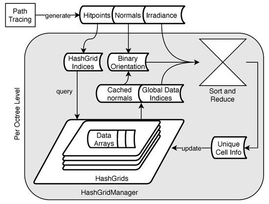
Figure 3.
An overview of the caching process. Hitpoints, normals, and irradiance samples are generated by the path-tracing process. The hitpoints’ coordinates are then used to determine the HashGrid indices for each hitpoint. Using these indices, the HashGridManager is queried for the global indices to the data arrays and the cached normals. A binary orientation for each irradiance sample, the actual irradiance sample, and the global data indices are now used to collate the data in a sort-and-reduce operation. The resulting unique information per grid cell is then merged with the current cache data.
During the caching process, rays are shot into the scene from the current camera view and traced along randomly generated paths , with being that path’s individual vertices located on scene surfaces, and being the maximal recursion depth. As we want to cache data not only for the first hitpoint (which would effectively only represent directly visible geometry), we compute illumination along subpaths with a maximum length of and store these for the first hitpoints. Thus, since all vertices of a path should account for the energy transported along the same number of consecutive vertices in order to provide consistent data, the maximum path length is , and the indirect illumination contributed to each vertex along the path has to be limited to the subpath vertices , . This is illustrated in Figure 4.
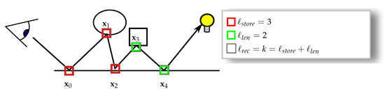
Figure 4.
Parameters for a single path. The parameter determines the maximum depth to which values are stored in the cache. After that depth, the illumination along subpaths is computed up to a maximum length of . The length of both determines the maximal recursion depth .
As soon as the local illumination and the reflected direction for the current vertex have been computed, the energy transported along the current path is updated by computing the throughput according to the locally evaluated BRDF. The first vertex along the current path that should still account for energy originating at the current vertex is at index . In order to take into account the accumulated throughput for the current subpath from vertex back to vertex , each preceding vertex is updated with the reflected local energy by computing the component-wise multiplication
Here, the diffuse material color is not accounted for in vertex . It is instead taken into account after reconstruction in order to avoid loss of spatial variation in the appearance of diffuse materials. All vertices from each path that belong to a Lambertian material are stored in the respective arrays indexed by the hash map. This includes diffuse illumination values , compressed normal vectors , the linear map index (only required if the hash map’s resolution R exceeds ), and the linear cell index , where and are necessary to store the data in our data structure correctly.
Now, the respective cells of the HashCache are updated with the newly computed light transport data. When updating the individual octree levels, the collected data are pre-accumulated before performing an update on the global data arrays in order to avoid synchronization issues. Pre-accumulation is implemented by first sorting the data using a radix sort approach and consecutively performing a reduction on the data with the global data index as the primary key and the binary orientation information (front or back) as the secondary key for both the sorting and reduction. In order to use the orientation information as the secondary key in the reduction, the individual sample’s normal vectors have to be replaced with binary front/back information: 1, if the sample lies within the front-facing hemisphere, and –1 otherwise. If storage is not an issue, more directions could be represented, which may also allow for caching glossy materials. Afterwards, the data are coarsened for the preceding octree level and the process is repeated until all levels have been updated. The full octree update is in , with n being the number of updated cache cells.
3.3. Reconstruction
As rendering scenes with Lambertian materials exclusively may cause them to appear visually dull and unrealistic, our system provides the means for handling materials with glossy or specular properties. An overview of the process described in this section is given in Figure 5, while a further description is given below.
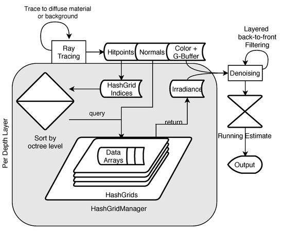
Figure 5.
An overview of the reconstruction process. A ray-tracing step is performed to find the actual hitpoints that have to be reconstructed from the cache. In order to support non-lambertian materials, this step includes tracing of rays until a diffuse surface is found, the background is hit, or a user-definable maximum recursion depth is reached. The HashGrid indices computed from the hitpoints are then sorted by the appropriate octree level, and the cache is queried for the actual data indices. Together with hitpoint-wise texture and geometry information, the acquired irradiance is filtered in a denoising step in a layered back-to-front way. This means that each recursion level is filtered individually and then combined with the next (closer) level, until the primary hitpoints are reached. The result is then combined in a running estimate to achieve higher image quality when the camera is not moving.
For the reconstruction step, primary geometry hitpoints are determined for each individual pixel, with the exception of glossy and specular materials, where the specific rays are traced further until they eventually arrive at maximum depth , a diffuse material, or hit the background. For each path, the accumulated throughput is stored for the first vertices as together with the diffuse material color, the local normal, and the appropriate octree level (selected by projecting the pixel area in object space). The reconstruction is executed per-level and accumulated in the image by selecting the correct orientation from each cell and multiplying the retrieved diffuse illumination value with .
In order to reduce the blocky appearance caused by low cache resolutions, we employ a spatial jittering method to compute the actual cell index. This jittering method is based on the hitpoint’s local tangent plane:
Here, and are the original and the jittered hitpoints, are uniformly distributed random numbers, and are the tangent and the binormal, is the actual cell size, and is the user-adjustable scale of the jittering. Finally, a basic edge-aware cross-bilateral denoiser filters remaining noise for each depth layer individually, and also tries to fill holes where cache information is not available.
Figure 6 shows the effect of jittering and denoising in two areas: While the wall in the back shows more high-frequency noise, the statue in the front reveals quantization artifacts due to the great differences between neighboring cache values. However, such artifacts are efficiently removed by the spatial jittering.
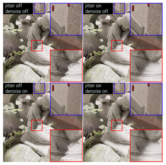
Figure 6.
Comparison of the same viewpoint rendered with all combinations of jittering and denoising. (Top left) HashCache-based reconstruction without any spatial jittering or denoising applied. (Top right) While spatial jittering cannot get rid of the high-frequency noise visible in the upper inset, it works well for hiding quantization artifacts. (Bottom left) Denoising alone does work well for fine-grained noise, but cannot remove quantization artifacts very well. (Bottom right) Combining jittering and denoising works well for both kinds of artifacts.
Note that spatial jittering may result in slight artifacts when cells are processed which do not have geometry in all neighboring cells that lie on the respective tangent plane (cf. Figure 7). This is mainly caused by the fact that our data structure does not support enhanced sparsity encoding, but rather relies on constrained access [51] to avoid further memory consumption. Two cases may appear:
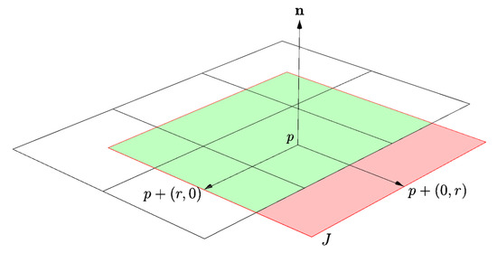
Figure 7.
Two-dimensional example of the possible issue with spatial jittering: For a hitpoint p on an arbitrary scene surface with a jitter radius of r, the sampled cell resulting from with and may not contain any scene geometry. Consequently, the according cell has no memory explicitly reserved in the hash map. The computed hash key may thus lead to empty or even plainly wrong cells. The filled area represents the set of possible jittered points J. The green area is the subset of points that result in valid keys, while the red area depicts the subset of invalid points.
- The hash key for the neighboring grid cell may belong to another cell that belongs to the scene’s geometry. In such a case, visual artifacts may occur.
- The hash key for the neighboring grid cell may yield an empty entry in the hash map. In this case, the irradiance value is set to the average of the pixel’s neighbors, i.e., invalid or unsampled pixels resulting from spatial jittering are filled in.
However, during our evaluation, we did not observe any major artifacts resulting from this. Thus, we decided not to include any way of querying a cell for its grid coordinates.
In Section 3.4, we present how we extend our system with a filtering approach that accounts for multiple bounces of glossy and specular reflections and refractions in order to improve visual quality. Note that in our implementation, caching and reconstruction are independent of each other. The caching process can be executed with an arbitrary sampling scheme at freely selectable resolutions, while the reconstruction just retrieves the stored illumination values from the data structure. Thus, the caching process may actually rely on arbitrary distributions of rays throughout the scene, which also enables strategies like randomly or adaptively sampling the scene along camera paths or creating importance-based sampling schemes. Additionally, the separate caching step can be performed with arbitrary numbers of samples. In our case, we tested the caching performance at various resolutions, as shown in Section 4.
3.4. Layered Filtering
While the plain octree reconstruction described so far may suffice in some scenarios, it is known from regular path tracing that convergence can be slow in many scenes. This makes it necessary to employ filtering methods in order to achieve noise-free images within an acceptable time frame. The kind of noise remaining in the generated images largely depends on the employed rendering method, while quantization artifacts are effectively reduced by the aforementioned spatial jittering method. However, it is important to note that the existing filtering methods developed for path tracing will not work for the kind of noise our approach exhibits, as noise scales with the distance to a surface because of the limited cache resolution. Our suggested filtering approach aims to increase visual fidelity under such circumstances, while explicitly accounting for glossy, specular, and refractive materials.
The main idea of our method is to split the traditional filtering step that is carried out on the final image into multiple steps by filtering each bounce of light in an individual layer (cf. Figure 8). With a non-layered filtering approach, the scene information available to the actual algorithm is limited to the first hitpoint, and multiple bounces between reflective and refractive materials have to be processed with the information at hand. This may result in a loss of detail or the need for more samples in order to achieve satisfactory results.
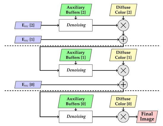
Figure 8.
Layered filtering process, illustrated for three layers. The reconstructed diffuse illumination for hitpoints that reached cached materials is added to the current result in each level. Together with the auxiliary buffers, such as the local G-buffer, it is then processed by the denoising method. Afterwards, albedo is taken into account, and the data are propagated to the next layer. This process is repeated until the first layer, formed by the primary hitpoints, is reached, and the final image is reconstructed.
At the core of our layered filtering approach is an arbitrary image-space denoising filter. In this exemplary case, this is a slightly extended cross-bilateral filter with a sparse sampling pattern based on the voxel filtering technique presented by Laine et al. [52]. In contrast to suggesting a concrete filtering method, we present a layered filtering framework, which is inherently independent of the filtering method used. This way, more recent filtering approaches could also be integrated and adapted to further improve the results. In order to provide the necessary information to this filter for each bounce of illumination, we expand upon the stored data described in Section 3.3. For each vertex belonging to the path , the following information is stored:
- Path segment length ,
- accumulated path length , serving as an extended depth buffer,
- geometric normal of the current vertex ,
- throughput for the next generated ray ,
- shininess of the current material ,
- reconstructed diffuse illumination , and
- diffuse material color (albedo) .
The edge-stopping functions we use are defined as follows:
As each bounce is filtered individually and the results are propagated, we omitted the depth index i from the description of the edge-stopping functions. The pixel indices are denoted p and q. Shininess is required to distinguish diffuse and glossy materials and apply adequate filter parameters. Albedo is required for preserving texture details, while throughput is required to apply the layered approach to non-diffuse materials properly. The parameters are user-defined scaling factors for normals, accumulated depth, local depth, color differences, and luminance differences, respectively. The color-based edge-stopping function has an additional weighting factor . The color difference is computed in L*a*b* color space. Generally, user-definable parameters have been chosen empirically by the best visual impression. The values used for the evaluation are mentioned in Section 4. Note that non-lambertian materials have a separate weighting factor for the color difference, which is not explicitly mentioned here.
All aforementioned information is available on a per-pixel, per-layer basis, which means that there is an actual image per light bounce (which we refer to as a layer). While later bounces of individual paths may arrive at different points in the scene, this is partially accounted for by using the accumulated ray depth as a filter guide. Although this yielded satisfactory results in our tests, there may be scene arrangements and material properties that cause this to be an issue. In such cases, we suggest using hitpoint world coordinates or HashGrid cell coordinates as possible additional filter guides.
Consequently, we process this data in a per-layer fashion, starting at the maximum bounce, filtering the result, and propagating it to the previous vertex of the path. Each time the filtered result is propagated from layer i to , it is multiplied with to account for the actual path throughput. The result is then added to the reconstructed diffuse illumination , and the accumulated image is filtered and propagated again until the primary hitpoints are reached. Additionally, after each layer has been filtered, it is multiplied with the local albedo in order to account for high-frequency content, as it is often contained in diffuse textures and shaders. Figure 9 shows the reconstructed diffuse illumination propagated from the third bounce to the secondary and then to the primary hitpoints.
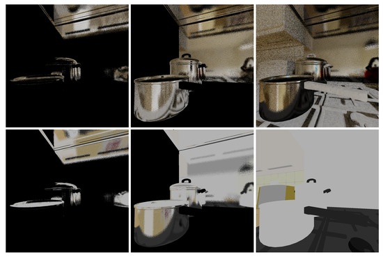
Figure 9.
Top: Unfiltered propagation of light bounces from the third hitpoint to the primary hitpoint (left to right). Bottom: The diffuse material colors (albedo) of each bounce above, multiplied after each filtering step. Note that non-diffuse materials appear white because they do not change the appearance of cached illumination values, which are strictly diffuse. The grey appearance of these materials resulted from tonemapping.
Our approach to caching, filtering, and accumulating is essentially an approximate final gathering step split into two separate steps: For diffuse materials, the illumination is approximated by integrating the energy arriving at each octree cell in the caching phase. For all non-lambertian materials, rays are traced until a diffuse material is hit in the reconstruction step. Then, the pre-gathered diffuse illumination is queried from the cache at these points. This hybrid approach is directly supported by our layered filtering method, which makes it possible to filter the illumination gathered in the octree cells separately based on local scene information, even if it is only indirectly visible in an image. Figure 10 shows a comparison between traditional and layered filtering for the first three bounces.
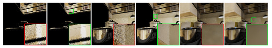
Figure 10.
Interleaved comparison between filtering the first three accumulated bounces with traditional (red insets) and layered filtering (green insets). The image has been reconstructed with one sample per pixel after filling the cache with four samples per pixel just for the illustrated viewpoint. The utilization of local geometry information through layered G-buffers shows clear improvements in image quality. Filter weights for color and luminance differences have been adjusted in comparison to the weights chosen in the evaluation measurements.
4. Results and Evaluation
In this section, we evaluate the visual quality, performance, and GPU memory requirements of the presented system. All measurements in this section were performed on a Linux system equipped with a GeForce GTX Titan X (Maxwell), a Core i7-7700 CPU, and 32 GiB of main memory. Scaling factors for the layered filtering were statically chosen to be , , , , , and . Images were rendered at a resolution of pixels.
4.1. Visual Quality
To determine the visual error, we rendered the scenes Country Kitchen (CK) and Streets of Asia (SoA) using a camera fly-through of 500 frames with different configurations of the HashCache and regular path tracing for comparison. On the one hand, standard path tracing was rendered for 1, 8, 64, 512, , and samples per pixel (spp) for both scenes and additionally for samples per pixel for Country Kitchen, as lower sample counts still revealed noise, especially in shadowed regions. The outputs with the highest sample counts are used as reference images for error computation. On the other hand, results using the HashCache system were generated with 1, 8, 64, and 512 spp with the presented reconstruction technique. The hash map resolution was chosen to be for CK and for SoA. All rendered images underwent the same tone-mapping process. The results illustrated in Figure 11 show a comparison of the visual quality measured as (top) the relative mean-square error (relMSE) and (bottom) the multi-scale structural similarity (MS-SSIM) [53] for varying sample counts. MS-SSIM mimics the multi-scale processing of the human visual system and is an important tool to judge image quality. The reuse of already-computed information in combination with a cross-bilateral filtering method already leads to the HashCache at 64 spp, yielding a quality similar to path tracing at 4,096 spp for the scene CK, even coming close to the reference image at 131,072 spp in the middle of the sequence. For SoA, the HashCache does not show an improvement in relMSE between 64 and 512 spp. At 64 spp, the relMSE is similar to path tracing at 512 spp. The scene SoA was rendered using a HashCache with a lower maximal resolution of only . As the spatial extent of the scene is high and the camera gets close to certain objects in the scene during the fly-through, quantization artifacts are likely to occur and to cause a larger difference between the reference solution and the cached irradiance. We expect even better quality at low sample densities when more advanced state-of-the-art filtering methods are integrated into our layered filtering framework. Nonetheless, they have to be adapted to the specific appearance of noise resulting from the HashCache (see Section 5).
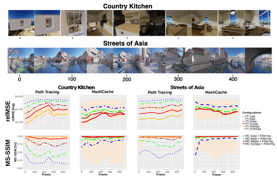
Figure 11.
Relative mean square error (relMSE, lower is better) and multi-scale structural similarity (MS-SSIM, higher is better) for the scene Country Kitchen (maximal build resolution ) and Streets of Asia (maximal build resolution ) at various sampling densities using path tracing and the HashCache system. The shaded area in the background outlines the respective relMSE and MS-SSIM ranges for the other rendering method for better comparison.
Applying a denoising method that is developed for standard path tracing is not suitable because of the visual appearance of noise in the HashCache, mainly because it appears at a scale that is larger than individual pixels. See Figure 12 for an example of noise appearance in our system. However, applying an additional denoiser on top of our filter may improve image quality even further by removing the fine-grained noise with which our method could not cope.
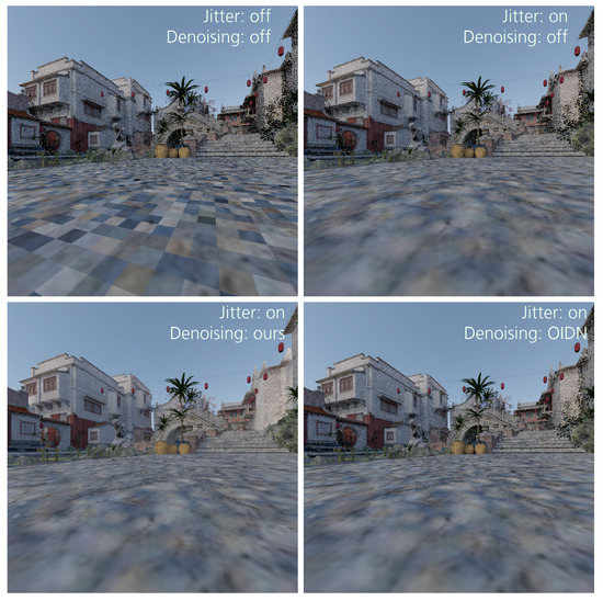
Figure 12.
The appearance of noise when using the HashCache. Without filtering and jittering, the distance-dependent scale of noise becomes clearly visible. Turning jitter on improves the visual appearance of quantization artifacts. Turning denoising on clearly improves regions with low sample counts, even filling in areas where no samples have been cached at all. The bottom right image shows the result with Intel’s Open Image Denoising (https://openimagedenoise.github.io/) instead of our denoiser. It becomes clear that the method cannot cope with the kind of noise exhibited by the HashCache.
Figure 13 shows a visual comparison of the quality improvements by increasing the hash resolution. Figure 6 shows the effectiveness of the spatial jittering method for hiding quantization artifacts. Figure 14 shows a comparison of images from three rendering modes: Pure path tracing, HashCache rendering an image sequence, and HashCache rendering an individual frame. Glossy reflections appear at a high quality early in the process, and details in such reflections are preserved very well. Figure 15 shows how well our system performs with a reflective surface. Due to the layered filtering approach, a quality similar to the reference rendering is already achieved with a fraction of the samples’ regular path-tracing needs. The effect of layered filtering for glossy and specular (refractive) materials is shown in more detail in Figure 16. Overblurring of details in refractions and reflections is avoided by the layered approach. Instead, the diffuse surface hit by the reflected and refracted rays is filtered in its own layer, and it is then propagated along the path.
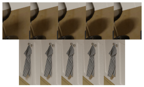
Figure 13.
The effect of adjusting the cache resolution. The rightmost pictures show the reference rendering at 131,072 spp. The rest of the images show cache resolutions from down to , decreasing by powers of two (from right to left). It can be seen that the decreased spatial resolution leads to quantization artifacts which are effectively filtered by jittering and denoising. However, fine-grained details would not be resolvable at low resolutions, and a complete loss of spatial details may occur.

Figure 14.
Comparison of images generated with pure path tracing and with the support of HashCache. (Left) The full image subdivided horizontally into areas rendered with HashCache at 1, 8, 64, and 512 spp, as well as with Path Tracing at 131,072 spp. Insets in green are magnified on the right for the various settings. (Right) Zoomed-in rendering for comparison, rendered with Path Tracing, HashCache (with three more frames in the sequence rendered before), and HashCache individual (the camera position has been rendered without filling the cache in the preceding frames). For the upper inset, the HashCache system already yields a quality at 64 spp (512 spp for individual rendering) that is on-par with the path-traced image at 131,072 spp. However, the lower inset shows more artifacts than the reference, even at 512 spp, for the HashCache rendering. The main reason for this is that we tuned the denoising filter to maintain shadows. Different denoising methods used with our layered framework should be able to resolve this well.
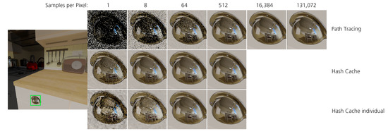
Figure 15.
Comparison of images generated with pure path tracing and with the support of HashCache. (Left) The full image rendered at the reference sample count of . The green inset is magnified on the right for the various rendering settings. (Right) Zoomed-in rendering for comparison, rendered with Path Tracing, HashCache (with four more frames in the sequence rendered before as a warm-up phase), and HashCache individual (without filling the cache in the preceding frames). For the upper inset, the HashCache system already yields a quality at 64 spp (512 spp for individual rendering) that is at least visually on-par with the path-traced image at 131,072 spp.
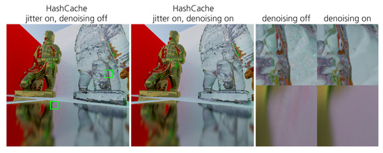
Figure 16.
The effect of layered filtering for glossy and specular materials. The cache was filled irregularly over 128 frames at 1 spp for a random fly-through. (Left) Unfiltered image at 128 reconstruction samples per pixel. (Center) Layered filtering at 128 reconstruction samples per pixel. (Right) Magnified insets. It is clearly visible how the noisy illumination from the back wall is reflected in the glossy surface on the ground when layered filtering is deactivated. With layered filtering, the noise can be filtered in a separate layer and then be accounted for in the glossy reflection. For the refractive material on the right, a similar effect is visible: Refracted rays pick up the noisy cache values from the back wall when layered filtering is deactivated. With layered filtering turned on, this noise can be effectively filtered before it is propagated to preceding vertices on the path. This allows for removing the noise locally without loss of details. An example for the individual layers being filtered is shown in Figure 10.
4.2. Performance
The rendering times and the average number of samples cached per frame for two different cache settings, and , are shown in Figure 17. The caching resolution factor (CRF) serves to adjust the number of rays cast in the caching phase. If set to 1, the number of primary rays will be the same as the chosen image resolution in the reconstruction step. While the cache construction times behave quadratically with regard to the CRF (because resolution is multiplied with the CRF both horizontally and vertically), reconstruction times do not depend on this setting. The average filtering time measured for the bilateral filter is 22 ms, while the cache query took 4.5 ms and the ray tracing phase for determining the visible geometry took around 31 ms. Thus, at a frame rate of around 17 fps, the reconstruction itself is well suited for interactive previews. The additional time taken by the caching procedure depends largely on the rendering and caching parameters. Setting low values for and causes the ray-tracing step to work not only with shorter, but also more coherent paths, which is beneficial for its performance. However, despite the top configuration delivering the fastest caching times, the number of updated cache cells on the right also shows that cache convergence should be expected to be relatively slow. Only storing the first vertex for each path also causes issues with glossy, specular, or transparent materials where the positions of subsequent vertices have not yet been seen directly by the user. Imagine a white wall reflected inside a mirror. It will only show a correctly rendered reflection if it has already been viewed before. However, this issue can be easily avoided by choosing a higher setting for , which is desirable anyway in order to cache illumination for scene parts that are not directly visible. The relatively slow cache update times for high CRF settings and high recursion and storage settings visible in Figure 17 are not a real issue for interactive exploration; in order to keep the process interactive, we modified our implementation to adjust the CRF to maintain a certain framerate while the camera is moving and only perform caching with the full resolution in the absence of movement. As shown in Figure 18, the actual reconstruction time is low enough to allow for fully interactive camera movements when the CRF is lowered. While the initial construction of the cache may take a couple of seconds depending on the set resolution, it is faster than Radiance Caching approaches [21,22]. Yet, this means that the HashCache is too slow to support fully dynamic scenes. We hope to omit the necessity of an explicit hash map construction step by using non-perfect hashing schemes in our future work.
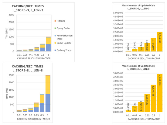
Figure 17.
Statistics for the scene Country Kitchen with different cache settings at a resolution of . (Left) Total rendering times, split into different steps. (Right) Average number of cells updated per frame of the 500 frame sequence. These numbers include the update of all octree levels. Note that the resolution factor can be adjusted dynamically to the current situation, e.g., when the user is moving.
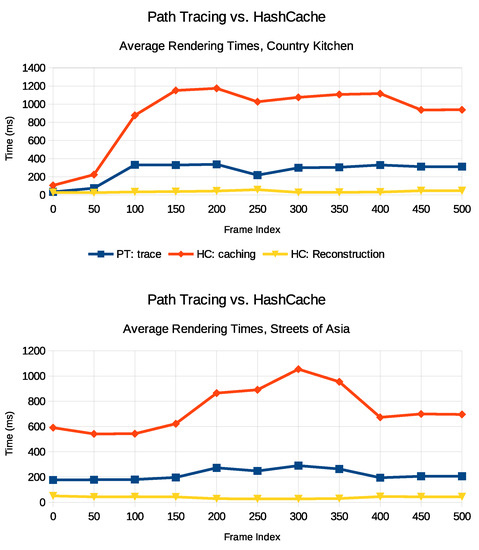
Figure 18.
Path-tracing and HashCache rendering times for Country Kitchen and Streets of Asia fly-throughs. Rendering time is given for 1 spp. PT: Trace is the time for pure path tracing at a maximum recursion depth of 8, HC: Caching is the caching part of HashCache computations which includes path tracing and cache updates, and HC: Reconstruction is the reconstruction part of the HashCache computations, which includes ray tracing, fetching the respective data from the cache, and reconstructing an image from the computed data (including filtering). While caching times are significantly higher than pure path-tracing times, data are reused between frames so that the actual caching resolution factor (CRF) can be reduced either permanently or deactivated during user input, allowing for smooth interaction.
4.3. Memory Requirements
The amount of required GPU memory for both the Country Kitchen and Streets of Asia scenes is shown in Table 1. While data density decreases by a factor of roughly 0.5 from level i to , memory requirements still increase by a factor of roughly 4 to 5. In total, the representation of Country Kitchen required an amount of 2.17 GiB for the data arrays and 406.92 MiB for the hash maps, while Streets of Asia required 691.37 MiB for the data arrays and 126.75 MiB for the hash maps at a total resolution of . One possible approach to handling the memory requirements resulting from higher resolutions is the integration of an out-of-core component into our system, dynamically loading currently required data from host memory to the GPU.

Table 1.
Data densities and memory requirements. The data density is the quotient of occupied cells and the actual number of cells for a full grid of resolution . Data memory is the amount of memory required to store the full data arrays. Hash memory is the amount of memory reserved for the hash map representation for the respective level.
4.4. Comparison to the State-of-the-Art
Methods such as the work by Schied et al. [40,41] have lower filtering run times (e.g., 4–5 ms on Titan X vs. 22 ms for the unoptimized HashCache filter) and produce a high visual quality, but cannot simply be applied to HashCache renderings because of the different appearance of noise. In addition, these techniques rely on a temporal coherence between subsequent views. In contrast, the HashCache allows for integration of GI data from arbitrary spatial locations. Thus, we are certain that all of these techniques can benefit from the knowledge from world-space caches. With the HashCache’s hybrid reconstruction method, specular materials can be supported with ease (see Figure 15). Notwithstanding, querying the world-space cache is slower than a cache in image space (4.5 ms for HashCache vs. ∼0.5–1 ms for Schied et al. [41]). Yet, in contrast to techniques such as NVIDIA’s machine learning solution [37] that needs specific training data or might produce inconsistent results, the HashCache can be filled at run time. Admittedly, the caching itself is a very costly operation (see Figure 18), but the CRF can be freely adapted. The figure also shows how the actual camera settings may influence caching and rendering times. For Country Kitchen, rendering at the beginning takes only a little time because the camera is still outside the room, which means that a lot of rays actually hit the background. As the camera gets nearer to the room, recursion depth increases because the rays are reflected between surfaces a lot more often. For the reconstruction, there is no vast difference caused by such a scenario. The only increase in recursion depth is caused by non-diffuse materials.
Once caches are filled to a certain extent, it is possible to limit the CRF largely and thus significantly reduce the cache update times. Moreover, the run time and caching behavior can be adapted dynamically to the user’s needs to stay within certain frame rate limits.
5. Conclusions and Outlook
In this paper, we presented a method for caching and reconstructing diffuse global illumination in a hash-based linkless octree to store illumination data for subsequent views. While the introduced reconstruction technique already produces images at a remarkable quality, it is possible to combine the the layered filtering framework with even more elaborate image-space filtering techniques to further enhance visual quality. We are certain that the HashCache can show its potential, especially in conjunction with methods that rely upon temporal integration in image-space, such as the work by Schied et al. [40,41], or other machine learning techniques, such as the work by Chaitanya [37]. However, the latter may require a new training set due to the more stable output produced by the HashCache and the noise appearing at different scales.
While we left out the rendering of specular-to-diffuse transport, using our system with a bidirectional path tracer would also allow for such paths to be handled more effectively. Though, when rendering high-frequency content such as caustics, the cache’s spatial resolution may be quickly exceeded. One option would be to provide a dynamic local caching mechanism that works at higher resolutions and adjusts to a scene’s light distribution. In addition, instead of storing each level of the octree in a separate hash map, we can store all levels in one hash map with occupation information. This approach avoids separate hash map queries per octree level, making it possible to compute the correct data array indices from the occupation information. However, memory requirements would increase.
Ultimately, we want to modify the caching method and employ a different hashing algorithm that allows for dynamic allocation on GPUs. This could avoid the necessity of data-structure rebuilds when geometry changes occur in a scene. In addition, we firmly believe that the HashCache can be a great tool to improve multi-view VR systems. Extending the system to support updates from multiple GPUs or even multiple machines, data quality throughout the scene could be improved in comparison to only caching illumination for the currently used perspective.
Author Contributions
Conceptualization, T.R. and P.B.; Data curation, T.R.; Investigation, T.R.; Methodology, T.R. and M.W.; Project administration, T.R.; Software, T.R. and M.W.; Supervision, P.B., A.H. and Y.L.; Validation, T.R.; Visualization, T.R.; Writing—original draft, T.R., M.W. and P.B.; Writing—review & editing, T.R. and M.W. All authors have read and agreed to the published version of the manuscript.
Funding
This work was supported by the German Federal Ministry for Economic Affairs and Energy (BMWi), funding the MoVISO ZIM-project under Grant No.: ZF4120902.
Conflicts of Interest
The authors declare no conflict of interest.
Abbreviations
The following abbreviations are used in this manuscript:
| BRDF | Bidirectional Reflectance Distribution Function |
| CK | Country Kitchen |
| CRF | Caching Resolution Factor |
| GI | Global Illumination |
| MC | Monte Carlo |
| MS-SSIM | Multi-Scale Structural Similarity |
| relMSE | Relative Mean-Square Error |
| SoA | Streets of Asia |
References
- Roth, T.; Weier, M.; Bauszat, P.; Hinkenjann, A.; Li, Y. Hash-based Hierarchical Caching for Interactive Previews in Global Illumination Rendering. Comput. Graph. Vis. Comput. 2019, 85–93. [Google Scholar] [CrossRef]
- Kajiya, J.T. The rendering equation. In Proceedings of the 13th Annual conference on Computer Graphics and Interactive Techniques, Dallas, TX, USA, 18–22 August 1986; pp. 143–150. [Google Scholar]
- Choi, M.G.; Ju, E.; Chang, J.W.; Lee, J.; Kim, Y.J. Linkless Octree Using Multi-Level Perfect Hashing. Comput. Graph. Forum 2009, 28, 1773–1780. [Google Scholar] [CrossRef][Green Version]
- Jensen, H.W. Global illumination using photon maps. In Rendering Techniques 96; Springer: Cham, Switzerland, 1996; pp. 21–30. [Google Scholar]
- Spencer, B.; Jones, M.W. Hierarchical Photon Mapping. IEEE Trans. Vis. Comput. Graph. 2009, 15, 49–61. [Google Scholar] [CrossRef] [PubMed]
- Binder, N.; Fricke, S.; Keller, A. Fast Path Space Filtering by Jittered Spatial Hashing. In ACM SIGGRAPH 2018 Talks; ACM: New York, NY, USA, 2018; pp. 71:1–71:2. [Google Scholar]
- Keller, A.; Dahm, K.; Binder, N. Path Space Filtering. In ACM SIGGRAPH 2014 Talks; ACM: New York, NY, USA, 2014; p. 66:1. [Google Scholar]
- Scherzer, D.; Yang, L.; Mattausch, O.; Nehab, D.; Sander, P.V.; Wimmer, M.; Eisemann, E. Temporal Coherence Methods in Real-Time Rendering. Comput. Graph. Forum 2012, 31, 2378–2408. [Google Scholar] [CrossRef]
- Ward, G.J.; Rubinstein, F.M.; Clear, R.D. A Ray Tracing Solution for Diffuse Interreflection. In Proceedings of the 15th Annual Conference on Computer Graphics and Interactive Techniques, Atlanta, GA, USA, 1–5 August 1988; pp. 85–92. [Google Scholar]
- Bala, K.; Dorsey, J.; Teller, S. Interactive Ray-Traced Scene Editing Using Ray Segment Trees. In Rendering Techniques’ 99; Lischinski, D., Larson, G.W., Eds.; Springer: Vienna, Austria, 1999; pp. 31–44. [Google Scholar] [CrossRef]
- Walter, B.; Drettakis, G.; Parker, S. Interactive Rendering using the Render Cache. In Rendering Techniques (Proceedings of the Eurographics Workshop on Rendering); Lischinski, D., Larson, G.W., Eds.; Springer-Verlag: Berlin, Germany, 1999; Volume 10, pp. 235–246. [Google Scholar]
- Ward, G.; Simmons, M. The holodeck ray cache: An interactive rendering system for global illumination in nondiffuse environments. ACM Trans. Graph. (TOG) 1999, 18, 361–368. [Google Scholar] [CrossRef]
- Sloan, P.P.; Kautz, J.; Snyder, J. Precomputed radiance transfer for real-time rendering in dynamic, low-frequency lighting environments. In Proceedings of the 29th Annual Conference on Computer Graphics and Interactive Techniques, San Antonio, TX, USA, 23–26 July 2002; pp. 527–536. [Google Scholar] [CrossRef]
- Tole, P.; Pellacini, F.; Walter, B.; Greenberg, D.P. Interactive global illumination in dynamic scenes. ACM Trans. Graph. (TOG) 2002, 21, 537–546. [Google Scholar] [CrossRef]
- Bala, K.; Walter, B.; Greenberg, D.P. Combining edges and points for interactive high-quality rendering. ACM Trans. Graph. (TOG) 2003, 22, 631–640. [Google Scholar] [CrossRef]
- Krivánek, J.; Gautron, P.; Pattanaik, S.; Bouatouch, K. Radiance Caching for Efficient Global Illumination Computation; INRIA: Rocquencourt, France, 2004. [Google Scholar]
- Christensen, P.H.; Batali, D. An Irradiance Atlas for Global Illumination in Complex Production Scenes. In Proceedings of the Fifteenth Eurographics Conference on Rendering Techniques, Grenoble, France, 21–23 June 2004; pp. 133–141. [Google Scholar]
- Dietrich, A.; Schmittler, J.; Slusallek, P. World-Space Sample Caching for Efficient Ray Tracing of Highly Complex Scenes; Technical Report; Computer Graphics Group, Saarland University: Saarbrücken, Germany, 2006. [Google Scholar]
- Gautron, P.; Bouatouch, K.; Pattanaik, S. Temporal Radiance Caching. IEEE Trans. Vis. Comput. Graph. 2007, 13, 891–901. [Google Scholar] [CrossRef] [PubMed]
- Brouillat, J.; Gautron, P.; Bouatouch, K. Photon-driven Irradiance Cache. Comput. Graph. Forum 2008, 27, 1971–1978. [Google Scholar] [CrossRef]
- Křivánek, J.; Gautron, P.; Pattanaik, S.; Bouatouch, K. Radiance Caching for Efficient Global Illumination Computation. IEEE Trans. Vis. Comput. Graph. 2005, 11, 550–561. [Google Scholar] [CrossRef]
- Omidvar, M.; Ribardière, M.; Carré, S.; Méneveaux, D.; Bouatouch, K. A radiance cache method for highly glossy surfaces. Vis. Comput. 2016, 32, 1239–1250. [Google Scholar] [CrossRef]
- Wang, R.; Wang, R.; Zhou, K.; Pan, M.; Bao, H. An Efficient GPU-Based Approach for Interactive Global Illumination; Association for Computing Machinery: New Orleans, LA, USA, 2009; pp. 1–8. [Google Scholar] [CrossRef]
- Hachisuka, T.; Jensen, H.W. Parallel Progressive Photon Mapping on GPUs; ACM: New York, NY, USA, 2010; p. 1. [Google Scholar]
- Crassin, C.; Neyret, F.; Sainz, M.; Green, S.; Eisemann, E. Interactive Indirect Illumination Using Voxel-Based Cone Tracing: An Insight; ACM: New York, NY, USA, 2011; p. 1. [Google Scholar]
- Thiedemann, S.; Henrich, N.; Grosch, T.; Müller, S. Voxel-based Global Illumination. In Symposium on Interactive 3D Graphics and Games; ACM: New York, NY, USA, 2011; pp. 103–110. [Google Scholar]
- Ritschel, T.; Dachsbacher, C.; Grosch, T.; Kautz, J. The State of the Art in Interactive Global Illumination. Comput. Graph. Forum 2012, 31, 160–188. [Google Scholar] [CrossRef]
- Scherzer, D.; Nguyen, C.H.; Ritschel, T.; Seidel, H.P. Pre-convolved Radiance Caching. Comput. Graph. Forum 2012, 31, 1391–1397. [Google Scholar] [CrossRef]
- Dammertz, H.; Sewtz, D.; Hanika, J.; Lensch, H. Edge-Avoiding A-Trous Wavelet Transform for fast Global Illumination Filtering. In Proceedings of the Conference on High Performance Graphics, Saarbrücken, Germany, 25–27 June 2010; pp. 67–75. [Google Scholar]
- Bauszat, P.; Eisemann, M.; Magnor, M.; Ahmed, N. Guided Image Filtering for Interactive High-quality Global Illumination. Comput. Graph. Forum 2011, 30, 1361–1368. [Google Scholar] [CrossRef]
- Gastal, E.S.L.; Oliveira, M.M. Adaptive Manifolds for Real-Time High-Dimensional Filtering. ACM Trans. Graph. (TOG) 2012, 31, 1–13. [Google Scholar] [CrossRef]
- Mara, M.; Luebke, D.; McGuire, M. Toward Practical Real-time Photon Mapping: Efficient GPU Density Estimation. In Proceedings of the ACM SIGGRAPH Symposium on Interactive 3D Graphics and Games, Orlando, FL, USA, 21–23 March 2013; pp. 71–78. [Google Scholar]
- Schwenk, K. Filtering Techniques for Low-Noise Previews of Interactive Stochastic Ray Tracing; Technische Universität Darmstadt: Darmstadt, Germany, 2013. [Google Scholar]
- Nguyen, C.H.; Scherzer, D.; Ritschel, T.; Seidel, H.P. Material Editing in Complex Scenes by Surface Light Field Manipulation and Reflectance Optimization. Comput. Graph. Forum 2013, 32, 185–194. [Google Scholar] [CrossRef]
- Zimmer, H.; Rousselle, F.; Jakob, W.; Wang, O.; Adler, D.; Jarosz, W.; Sorkine-Hornung, O.; Sorkine-Hornung, A. Path-space Motion Estimation and Decomposition for Robust Animation Filtering. Comput. Graph. Forum 2015, 34, 131–142. [Google Scholar]
- Munkberg, J.; Hasselgren, J.; Clarberg, P.; Andersson, M.; Akenine-Möller, T. Texture Space Caching and Reconstruction for Ray Tracing. ACM Trans. Graph. (TOG) 2016, 35, 249:1–249:13. [Google Scholar] [CrossRef]
- Chaitanya, C.R.A.; Kaplanyan, A.S.; Schied, C.; Salvi, M.; Lefohn, A.; Nowrouzezahrai, D.; Aila, T. Interactive Reconstruction of Monte Carlo Image Sequences Using a Recurrent Denoising Autoencoder. ACM Trans. Graph. (TOG) 2017, 36, 98:1–98:12. [Google Scholar] [CrossRef]
- Bako, S.; Vogels, T.; Mcwilliams, B.; Meyer, M.; NováK, J.; Harvill, A.; Sen, P.; Derose, T.; Rousselle, F. Kernel-predicting Convolutional Networks for Denoising Monte Carlo Renderings. ACM Trans. Graph. (TOG) 2017, 36, 1–14. [Google Scholar] [CrossRef]
- Silvennoinen, A.; Lehtinen, J. Real-time global illumination by precomputed local reconstruction from sparse radiance probes. ACM Trans. Graph. (TOG) 2017, 36, 1–13. [Google Scholar] [CrossRef]
- Schied, C.; Kaplanyan, A.; Wyman, C.; Patney, A.; Chaitanya, C.R.A.; Burgess, J.; Liu, S.; Dachsbacher, C.; Lefohn, A.; Salvi, M. Spatiotemporal Variance-guided Filtering: Real-time Reconstruction for Path-traced Global Illumination. In Proceedings of the High Performance Graphics, Los Angeles, CA, USA, 28–30 July 2017; pp. 2:1–2:12. [Google Scholar]
- Schied, C.; Peters, C.; Dachsbacher, C. Gradient Estimation for Real-time Adaptive Temporal Filtering. Proc. ACM Comput. Graph. Interact. Tech. 2018, 1, 24:1–24:16. [Google Scholar] [CrossRef]
- Binder, N.; Fricke, S.; Keller, A. Massively Parallel Path Space Filtering. arXiv 2019, arXiv:1902.05942. Available online: https://arxiv.org/abs/1902.05942 (accessed on 14 February 2020).
- Hirvonen, A.; Seppälä, A.; Aizenshtein, M.; Smal, N. Accurate Real-Time Specular Reflections with Radiance Caching. In Ray Tracing Gems: High-Quality and Real-Time Rendering with DXR and Other APIs; Haines, E., Akenine-Möller, T., Eds.; Apress: Berkeley, CA, USA, 2019; pp. 571–607. [Google Scholar] [CrossRef]
- Luksch, C.; Wimmer, M.; Schwärzler, M. Incrementally baked global illumination. In Proceedings of the ACM SIGGRAPH Symposium on Interactive 3D Graphics and Games, Montreal, QC, Canada, 21–23 May 2019; pp. 1–10. [Google Scholar] [CrossRef]
- Wang, Y.; Khiat, S.; Kry, P.G.; Nowrouzezahrai, D. Fast non-uniform radiance probe placement and tracing. In Proceedings of the ACM SIGGRAPH Symposium on Interactive 3D Graphics and Games, Montreal, QC, Canada, 21–23 May 2019; pp. 1–9. [Google Scholar] [CrossRef]
- Yalçıner, B.; Sahillioğlu, Y. Voxel transformation: Scalable scene geometry discretization for global illumination. J. Real-Time Image Process. 2019. [Google Scholar] [CrossRef]
- Zhao, Y.; Belcour, L.; Nowrouzezahrai, D. View-dependent Radiance Caching. In Proceedings of the 45th Graphics Interface Conference on Proceedings of Graphics Interface 2019, Kingston, ON, Canada, 28–31 May 2019; Canadian Human-Computer Communications Society: Kingston, ON, Canada; pp. 1–9. [Google Scholar] [CrossRef]
- Huo, Y.; Wang, R.; Zheng, R.; Xu, H.; Bao, H.; Yoon, S.E. Adaptive Incident Radiance Field Sampling and Reconstruction Using Deep Reinforcement Learning. ACM Trans. Graph. (TOG) 2020, 39, 6:1–6:17. [Google Scholar] [CrossRef]
- Alcantara, D.A.F. Efficient Hash Tables on the GPU. Ph.D. Thesis, University of California, Davis, Davis, CA, USA, 2011. [Google Scholar]
- Pérard-Gayot, A.; Kalojanov, J.; Slusallek, P. GPU Ray Tracing Using Irregular Grids. Comput. Graph. Forum 2017, 36, 477–486. [Google Scholar] [CrossRef]
- Lefebvre, S.; Hoppe, H. Perfect Spatial Hashing. ACM Trans. Graph. (TOG) 2006, 25, 579–588. [Google Scholar] [CrossRef]
- Laine, S.; Karras, T. Efficient Sparse Voxel Octrees. IEEE Trans. Vis. Comput. Graph. 2011, 17, 1048–1059. [Google Scholar] [CrossRef]
- Wang, Z.; Simoncelli, E.P.; Bovik, A.C. Multiscale structural similarity for image quality assessment. In Proceedings of the Thirty-Seventh Asilomar Conference on Signals, Systems & Computers, Pacific Grove, CA, USA, 9–12 November 2003; pp. 1398–1402. [Google Scholar]
© 2020 by the authors. Licensee MDPI, Basel, Switzerland. This article is an open access article distributed under the terms and conditions of the Creative Commons Attribution (CC BY) license (http://creativecommons.org/licenses/by/4.0/).