Abstract
The Sensing as a Service is emerging as a new Internet of Things (IoT) business model for sensors and data sharing in the cloud. Under this paradigm, a resource allocation model for the assignment of both sensors and cloud resources to clients/applications is proposed. This model, contrarily to previous approaches, is adequate for emerging IoT Sensing as a Service business models supporting multi-sensing applications and mashups of Things in the cloud. A heuristic algorithm is also proposed having this model as a basis. Results show that the approach is able to incorporate strategies that lead to the allocation of fewer devices, while selecting the most adequate ones for application needs.
1. Introduction
For the Internet of Things (IoT) not to become just a collection of Things, unable to be discovered, a move towards the Web of Things (WoT) is required. The WoT aims to bring real-world objects into the World Wide Web and is envisaged as the key for an efficient resource discovery, access and management [1,2]. This way, objects become accessible to a large pool of developers and mashups combining physical Things with virtual Web resources can be created. However, as more and more physical Things become available in the IoT world, and mashups are built, large amounts of data with processing needs will emerge, meaning that new challenges arise in terms of storage and processing. The Sensing as a Service (Se-aaS) model, relying on cloud infrastructures for storage and processing, emerges from this reality [3,4].
The Se-aaS is a cloud-based service model for sensors/data to be shared, allowing for a multi-client access to sensor resources, and multi-supplier deployment of sensors [3]. This way, everyone can benefit from the IoT ecosystem, while benefiting from cloud’s storage and processing capabilities. When incorporating Se-aaS platforms in the application architecture, software components usually have bindings to virtual sensors managed in the cloud. Any workflow, wiring together virtual sensors, actuators and services from various Web sources, is managed on the client side. Managing these mashups at the client side brings, however, significant delays because there will be multiple travelings of data to the client. The proposal in this article is for software components to be able to have bindings to mashups managed in the cloud. The cloud would ensure that events are processed and actuations are triggered, according to the predefined workflow of the mashup, delivering just the final data of interest to the consumer/client application. The whole mashup, or parts of it, may also be consumed by multiple applications. Managing mashups in the cloud brings new challenges when assigning resources (devices and cloud) to consumer needs, as discussed in the following sections. The main contributions of this article are the following:
- Resource allocation model for sensor clouds under the Se-aaS paradigm, assuming that applications have bindings to mashups managed in the cloud;
- Heuristic algorithm having the just mentioned model as a basis.
The proposed model is adequate for many emerging IoT Se-aaS business models, like the ones supporting multi-sensing applications, mashups of Things, and/or integration of data from multiple domains, allowing for a more efficient orchestration of both sensor and cloud resources to face client requests.
The remainder of this article is organized as follows. In Section 2, cloud-based Se-aaS architectures and system functionalities are discussed. Section 3 discusses work related with the Se-aaS paradigm. Section 4 presents the resource allocation model, and a heuristic algorithm is proposed. Results are analysed in Section 5 and Section 6 concludes the article.
2. Cloud-Based Sensing-as-a-Service
Many cloud-based “as a service” models have emerged over the last several years. The most relevant are: (i) Infrastructure as a Service (IaaS), providing computing resources (e.g., virtual machines); (ii) Platform as a Service (PaaS), providing computing platforms that may include operating system, database, Web server, and others; and (iii) Software as a Service (SaaS), where the cloud takes over the infrastructure and platform while scaling automatically [5]. All of these models promote the “pay only for what you use”. The Se-aaS model emerged more recently and the idea is for sensing devices, and their data, to be shared in the cloud, so that many parties can use them. This means that there is a multi-supplier deployment of sensors, and multi-client access to sensor resources. Se-aaS platforms may provide storage, visualization and management facilities [6]. Naturally, cloud service providers must compensate the device owners for their contribution, or find some incentive mechanism for them to participate [7,8]. Secure user-centric service provisioning is also a critical issue [9].
2.1. Architecture
Similarly to other cloud-based “as a service” models, the resources in Se-aaS should be dynamically provisioned and de-provisioned on demand. Since sensors (or data) are to be accessed by multiple users/applications in real time, through service subscription, the costs associated with owing, programming and maintaining sensors and/or sensor networks will scale down [9]. Figure 1 shows the service architecture of a Se-aaS system. The challenges when planning and designing such systems are:
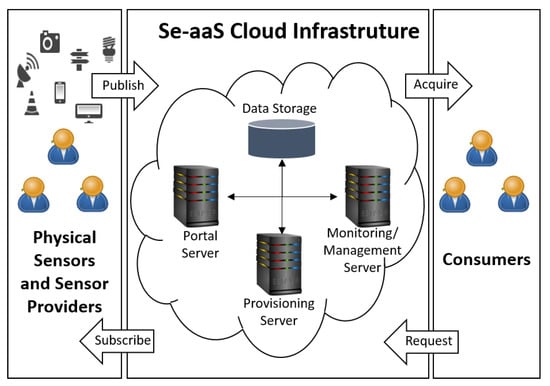
Figure 1.
Se-aaS architecture.
- Underlying complexity should be hidden, so that services and applications can be launched without much overhead;
- Scalability, ensuring a low cost-of-service per consumer while avoiding infrastructure upgrade;
- Dynamic service provisioning for pools of resources to be efficiently used by consumers.
2.2. System Functionalities
Besides registration capabilities for consumers and providers, IoT Se-aaS systems end up having one or more of the following functionalities [4]:
- Virtualization: Sensor virtualization is used to enable the management and customization of devices by clients/applications/consumers, allowing a single device to be linked to one or multiple consumers. Groups of virtual sensors can be made available for specific purposes. Virtualization is illustrated in Figure 2.
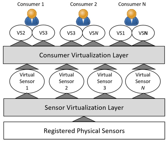 Figure 2. Virtualization layers in Se-aaS.
 - Dynamic Provisioning: This allows consumers to leverage the vast pool of resources on demand. A virtual workspace (e.g., virtual machine) is usually created for the provisioning of virtual sensors, which can be under the control of one or more consumers. Virtual workspace instances are provisioned on demand, and should be as close as possible to the consumer’s zone.
- Multi-Tenancy: A high degree of multi-tenancy in architectures allows sharing of sensors and data by consumers, and dedicated instances for each sensor provider. Issues like scaling according to policies, load balancing and security need to be considered.
2.3. Embedding Mashups into the Cloud
The virtualization approach shown in Figure 2 allows sensors/data to be accessed and mashups to be built at the client side. As an example, an application may use data from VS1 and VS3 to decide on some actuation. However, if such workflows (wiring together VSs, actuators and services from various Web sources) were implemented in the cloud, some of the data would not have to travel to the client side. The cloud would ensure that events are processed and actuations are triggered, according to the predefined workflow of mashups, delivering just the final data of interest to the consumer/client application. The whole mashup, or parts of it, may also be consumed by multiple applications. This additional system functionality results in an additional mashup virtualization layer, as illustrated in Figure 3.
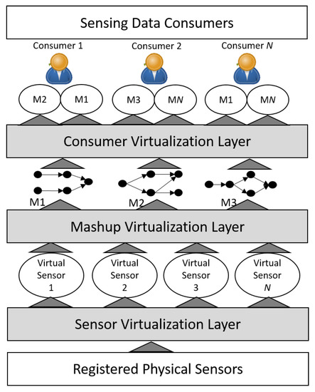
Figure 3.
Virtualization layers in Se-aaS architectures having mashups embedded into the cloud.
Managing mashups in the cloud brings new challenges when assigning resources (devices and cloud) to consumer needs. More specifically, mashups end up defining flow dependencies (see Figure 3), which will influence:
- Mapping between one or more mashup elements (defined by consumers) and a virtual Thing, for resource optimization.
- Mapping between virtual Things and physical Things (materialization onto devices).
- Placement of virtual Thing workspaces in the cloud.
Thus, after mapping a virtual Thing to one or more mashup elements, such virtual Thing ends up participating in multiple mashups. The just mentioned mappings should be done having some criteria in mind, like an efficient use of physical Things and cloud resources, a reduction of flows or delay between virtual Thing workspaces (imposed by mashups), which improves user’s quality of experience and scalability. This approach fits many emerging IoT Se-aaS business models, like the ones supporting multi-sensing applications, mashups of Things, and/or integration of data from multiple domains. Note that the approach in Figure 2 will be a particular case of Figure 3 where mashups have a single element.
3. Related Work
The Se-aaS concept was initially introduced by [7,10], where cloud-based sensing services using mobile phones (crowd sensing) are discussed. The authors identify the challenges of designing and implementing such systems. The general idea of these proposals is to use the sensors of mobile devices to fulfil some need/request. In the context of smart cities, Se-aaS is discussed in [3,11]. The first addresses technological, economical and social perspectives, while the last proposes the abstraction of physical Things through semantics, so that these can be integrated by neglecting their underlying architecture. In [12,13], the semantic selection of sensors is also addressed. Multimedia Se-aaS have been explored in [14,15,16,17]. These mainly focus on real-type communication requirements of audio/video data, and Wang et al. [16] explores cloud edges and fogs.
Regarding virtualization of devices, several proposals have appeared in the literature. When virtualizing Wireless Sensor Networks (WSNs), the general idea is that the cloud should abstract different physical device platforms in order to give the impression of a homogeneous network, enhancing user experience when configuring devices. In [6,18,19], data storage and/or device assignment to tasks is discussed, allowing for a uniform and widespread use of WSNs. In [6], a WSN virtualization model is discussed. Service-centric models in [20,21,22] focus on the services provided by a WSN acting as a service provider.
In IoT Se-aaS business models, the general idea is to virtualize sensing services provided by devices. A virtual sensor ends up being responsible for passing user’s specifications to device(s) and for processing of the sensed data before delivering it to users. In [23,24], the physical resources are abstracted, virtualized, and presented as a service to the end users. This way, the access and interaction with physical Things becomes uniform and in compliance with IoT/WoT goals. Specific platforms providing efficient sharing mechanisms for data (among multiple applications) have been proposed in [4,25,26]. In [4], the extra challenge is multitenancy considering both sensor providers and consumers, and on-demand big data sensing service. In [25], the focus is on how to ensure an ecosystem that is interoperable at multiple layers, for the Fog and Edge Computing paradigms to be explored. Such paradigms are suitable when latency, bandwidth utilization and energy consumption need to be reduced, but, for high-demanding processing tasks and integration of data from multiple sources, the use of the cloud is inevitable [27].
In this article, and contrarily to other works, consumer/client applications have bindings to mashups managed in the cloud, each mashup combining one or more Things through some workflow. This approach avoids the delay that exists when mashups are managed at the client side because the traveling of data to the client is significantly reduced. As far as is known, mashups have not been considered in previous Se-aaS cloud works.
4. Resource Allocation Model
4.1. Definitions and Assumptions
Definition 1 (Physical Thing).
A sensor detecting events/changes, or an actuator receiving commands for the control of a mechanism. The model of a physical Thing i includes all properties necessary to describe it, denoted by , and all its functionalities, denoted by . That is, and , where is the overall set of properties (e.g., sensing range, communication facility, energy consumption, location), and the overall set of functionalities (e.g., image sensor), from all devices registered in the cloud.
It is assumed that properties and functionalities, at and , are semantic-based. That is, specific vocabularies are used when naming properties and functionalities (see [28]). In addition, each property will have a “subject/predicate/object” description (A Resource Description Framework (RDF) triple. See https://www.w3.org/standards/semanticweb/) associated with it (e.g., cameraResolution hasValue 12.1 MP) denoted by . The set of all registered physical Things is denoted by , and it is assumed that providers voluntarily register/deregister physical Things to/from the cloud.
Definition 2 (Virtual Thing).
Entity used for the mapping of multiple mashup elements (consumers) to physical Things, having a virtual workspace associated it. A virtual Thing j can be materialized through one or more concerted physical Things, denoted by , . Therefore (the symbol ≜ means equal by definition, in our case logically/semantically equivalent), and . A virtual Thing materialization must fulfill the requirements of all its consumers.
Thus, a virtual Thing can have in background one or multiple physical Things working together to provide the requested functionality, producing data that reaches the cloud using standard communication. The set of virtual Things created by the cloud is denoted by .
The set of all consumer applications is denoted by , and these are assumed to be outside the cloud. An application can have one or more independent components, denoted by , and each component has a binding to a mashup in the cloud.
Definition 3 (Mashup).
Workflow wiring together a set of elements/nodes. Each element n included in a mashup has a functionality requirement and a set of property conditions, denoted by and , respectively.
That is, it is assumed that user application components have bindings to mashups stored in the cloud, each mashup including elements connected by a workflow (Web templates can be used to draw mashups). The output of a mashup element can be input to another, while final mashup output data is sent to the corresponding application component. The functionality requested by a mashup element, and property conditions, are also semantic-based and each has a “subject/predicate/object” description of the condition that is being defined (e.g., cameraResolution greaterThan 12.1 MP; frequencySampling equalTo 10 s), denoted by . Thus, mashup elements are not physical Things, but, instead, nodes that specify requirements. The overall population of mashup elements (from all applications) is denoted by .
Virtual Things, to be created in the cloud, are the ones to be materialized into physical Things. Then, each mashup element must be mapped to a single virtual Thing, while a virtual Thing can be mapped to multiple mashup elements (with same functionality and compatible property requirements). With such approach, data generated by a virtual Thing can be consumed by multiple application mashup elements, reducing data collection/storage and increasing the usefulness of data. The right set of virtual Things to be created in the cloud, their mapping to mashup elements and their materialization onto physical Things should be determined while using resources efficiently, which is discussed in the following section.
The goal of cloud virtualization is for users to remain unaware of physical devices involved in the process. This way, physical Things can be dynamically allocated to virtual Things used by applications. The client ends up having no deployment and maintenance costs, while having an on-demand fault tolerant service because virtual Things can always use other available physical Things. Clients would not be aware of such change due to virtualization.
4.2. Formalization
Let us assume a particular partition of (population of mashup elements), denoted by , where all elements in a have the same functionality requirement. A virtual Thing mapped to must provide the requested functionality, which is the same for all mashup elements in . The following allocation function can be defined:
One or more physical Things materialize one virtual Thing. Assuming to be a specific partition of , each making sense from a functional point of view, the function is defined for virtual Thing materialization:
This states that a virtual Thing is materialized by , including one or more physical Things, if they are functionally similar.
Different partitions, and allocations done by f and g, have different impacts on the use of resources (cloud and physical Things) and provide different accomplishment levels for property requirements (more or less tight). Therefore, the best partitions should be determined. Let us assumed that is the universe set including all feasible partitions of mashup elements, . That is, and , . Also assume that is the universe set including all feasible partitions of physical Things, . That is, and , . The impact of f and g allocations, regarding the gap between requirements and properties of physical Things, can be described by the following cost function :
where includes all properties, having conditions, from mashup elements in . For each property , the is used to capture the lowest gap between requirements and physical Things regarding property p (e.g., if two elements in request for 12.1 MP and 24.2 MP camera resolutions, respectively, and the materialization of ’s virtual Thing is a physical Thing providing 48.4 MP, then the 24.2 to 48.4 MP gap is the request-supply gap to be considered; the other request is considered to be fulfilled). Note that returns the virtual Thing assigned to . Since multiple physical Things can be associated with a virtual Thing materialization, the at Equation (3) must be defined by:
where provides the gap between the property requirement and property value at one of the physical Things enrolled in materialization. Multiple physical Things may include a property and, therefore, is used to capture the highest gap value, in order to avoid virtual Thing materializations from having physical Things with property values far above the requirements. All the just mentioned gaps can be determined using SPARQL semantic query language (See https://www.w3.org/TR/rdf-sparql-query/) [29,30]. Having the previous definitions in mind, the best partitioning for and , determining which virtual Things should be built and their materialization, could be given by . This would provide scalable solutions because the number of required virtual Things (and virtual workspaces) ends up being minimized (see Equation (3)). However, mashups define flows between their elements. This means that, after mapping partitions of (mashup elements) into virtual Things, there will be flows between virtual workspaces of virtual Things. These flows must be taken into account so that scalability and QoE are not jeopardized due to overhead and delay in the cloud. Therefore, an additional cost function is defined as:
where:
- is a physical-to-virtual (P2V) transfer cost associated with the flow of data from physical Things to virtual Thing’s workspace in the cloud. This is zero if , meaning that is not used in the materialization of ’s virtual Thing;
- is a virtual-to-virtual (V2V) transfer cost associated with the flow of data between virtual Things’ workspaces of partitions and . This is zero if no flow between workspaces is required;
- is a virtual-to-application (V2A) transfer cost associated with flow of data from virtual Things’ workspaces to user applications. This is zero if the application is supposed to consume such data.
Transfer costs may reflect the number of hops and/or processing needs at these hops, meaning that it is dependent on the placement of virtual workspaces in the cloud. A Cloud Service Provider (CSP), which will be denoted by , often includes a set of distributed networks, that interconnect to provide services, and are usually organized in order to better serve certain regions. Therefore, a CSP is defined by , where includes a set of computing resources that can host virtual workspaces.
Finally, the best resource allocation, or partitioning for and , is defined by:
where and are weights, , defining the relative importance of normalized (Normalization formula: ) costs, and .
4.3. Resource Allocation Algorithm
Based on the previous model, a resource allocation algorithm is proposed next. It is assumed that:
- As physical Things are registered in the cloud, a pool of possible materializations is computed for each functionality, denoted by , using SPARQL. A materialization may involve one or more registered physical Things, and a physical Thing may be at multiple pools.
- As application mashups are inserted in the cloud, an auxiliary graph is updated. The includes all mashup elements, are the links denoting a flow between two elements of a mashup, and are compatibility links between two elements from any mashup. That is, a link between and exists in if: (i) nodes have the same functionality requirement; and (ii) property requirements are compatible (SPARQL is used to determine compatibility).
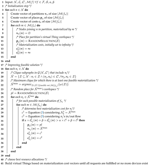
The resource allocation algorithm is described in Algorithm 1. The initialization step builds a partition for each mashup element, generates random places in CSP resources for them, and assigns an infinite cost. This has to be done in a per materization basis because different materializations involve different physical Things, generating different costs, and some materializations may not even be feasible due to mashup element property conditions. For random placement of partition’s virtual Thing workspace, a uniform distribution is used for load balancing to be obtained in the long term. The second step improves this initial solution by analysing cliques in auxiliary graph , and materialization possibilities.
For the last step, different selection criteria have been compared: (i) cheapest materialization cost (CMC) first; (ii) cheapest materialization, of mashup element (node in graph in ) with fewer materialization choices (LMC), first; (iii) cheapest materialization, of mashup element with highest cost variance (HCV), first. The reasoning behind LMC is that more materializations might be possible if critical mashup elements are processed first. Regarding HCV, the reasoning is that a late selection of mashup elements with highest cost variance might result in materializations with higher cost.
| Algorithm 1: Resource allocation heuristic |
 |
5. Performance Analysis
5.1. Scenario Setup
To carry out evaluation, a pool of functionalities was created together with a pool of properties for each functionality. Based on these, physical Things and mashup elements were created as follows:
- Mashups were randomly generated using the algorithm in [31], which is suitable for the generation of sparse sensor-actuator networks. An average of 10 elements per mashup is defined.
- The functionality required by each mashup element is randomly selected from the pool of functionalities, together with 50% of its properties. Each pair sharing the same functionality requirement is assumed to be compatible with probability .
- A physical Thing has a functionality assigned to it, together with 50% of its properties (randomly extrated from corresponding pool).
- The gap between a property condition and device property is randomly selected from , where is the lowest cost and is the highest (moderate and extreme levels).
This information is used to generate random scenarios, from which results are extracted. Regarding the CSP network graph, this was randomly generated assuming (number of places with computing resources that can host virtual workspaces) and a network density (Network density is measured using , where L is the number of links and N is the number of nodes) of 0.25. Tests include and values equal to 0.25 or 0.75, , so that the impact of component costs in (6) can be evaluated. Table 1 summarizes the adopted parameter values. All simulations were performed using C++ programming language.

Table 1.
Adopted parameter values.
5.2. Results
5.2.1. Materializations and Fulfilled Mashup Elements
The plots in Figure 4, Figure 5 and Figure 6 show how CMC, LMC and HCV strategies perform regarding the number of materializations (number of virtual Things materialized into physical devices), number of elements from mashups that have been fulfilled (mapped to a virtual Thing and, therefore, materialized into a physical device) and the average number of mashup elements per virtual Thing (average size of clique at Algorithm 1). From such plots, it is possible to observe that the worst strategy is LMC that reaches the total number of available devices more quickly while fulfilling fewer mashup elements than the other strategies. This is confirmed by the relatively low average number of mashup elements mapped to virtual Things (low aggregation level). The approach of LMC is to choose the cheapest materialization from mashup elements with fewer materialization choices, based on the assumption that more materializations would be possible if critical mashup elements were processed first. However, such mashup elements end up being the ones with more incompatible requirements (reason behide having fewer materialization choices), leading to a less efficient use of physical devices. That is, for a specific number of mashups, more devices are used for materialization of virtual Things having a low level of aggregation.
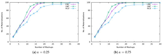
Figure 4.
Number of virtual Things materialized into physical Devices.
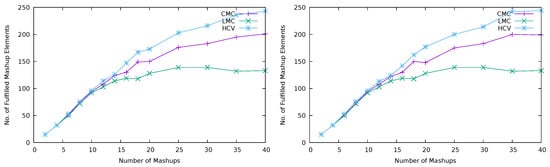
Figure 5.
Number of fulfilled mashup elements.
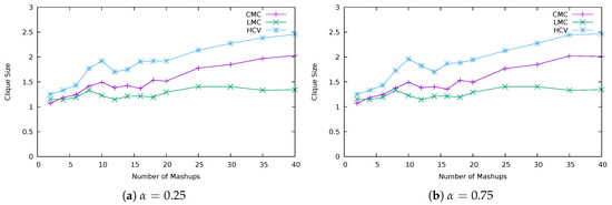
Figure 6.
Average number of mashup elements per virtual Thing.
The best strategy is HCV that presents a higher average number of mashup elements mapped to virtual Things, when compared with the other strategies, and more fulfilled mashup elements. Such highest aggregation level leads to a more controlled use of available devices, which are not wasted with materialization of virtual Things having a low level of aggregation. The approach of HCV is to pick the cheapest materialization from mashup elements with highest cost variance. This is based on the assumption that their late selection could result in a materialization with high cost. It happens that a mashup element having high cost variance also means that such mashup element has more requirements that are compatible with others, leading to a higher level of aggregation. For this reason, HCV presents better results.
Note that, for a relatively low number of mashups, the difference between strategies, regarding the number of virtual Things materialized into devices and fulfilled mashup elements, is very low. This is because the population of mashup elements is small, not allowing a high level of aggregation. That is, it is more difficult to find mashup elements with compatible requirements, for these to be linked to the same virtual Thing.
Regarding the impact of changing , which is the importance given to the cost associated with the gaps between the mashup element’s properties and physical Thing’s properties, it looks like this does not influence the number of virtual Things materialized into devices and fulfilled mashup elements.
5.2.2. Cost
The plots in Figure 7 show the overall materialization cost resulting from CMC, LMC and HCV strategies, together with the two cost components associated with Equations (3) and (5), and in Algorithm 1, respectively. Plots show that, when the number of devices in use is not close to the limit, the highest cost is the one given by LMC because of its low aggregation level (low average number of mashup elements mapped to virtual Things). HCV ends up providing the best cost values because it makes more aggregations. More specifically, the in Equation (3) captures the lowest gap between requirements of mashup elements (linked to a virtual Thing) and physical Things, reducing the overall cost.
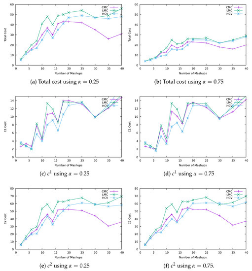
Figure 7.
Materialization cost.
After all the devices are in use; however, CMC is the one able to reduce the overall cost because it has the freedom to search for the cheapest cost, while the other strategies are conditioned in the search. LMC must pick the cheapest cost from mashup elements with fewer materialization choices, while HCV must pick the cheapest cost from mashup elements with highest cost variance. Although the population of mashup elements is greater, CMC does not improve its overall cost thanks to component (related with gaps between the mashup element’s properties and physical Thing’s properties) because this strategy has a low aggregation level. Instead, the reduction is achieved thanks to component, meaning that better placements for virtual Things, reducing the number of hops between workspaces, were found. LMC and HCV strategies were not able to reduce because these strategies are conditioned in their search for the cheapest materialization, as just mentioned.
Regarding the impact of , it is possible to conclude that strategies present more similar costs when has more importance than () because of the just mentioned improvement of by CMC. Note that HCV presents the best results on , when compared with the other strategies, being able to make more aggregations without increasing the materialization cost. This strategy may, however, be improved in the future for better virtual Thing placements to be found, as its does not reduce as in CMC.
5.2.3. Number of Flows
From the number of flows between virtual Thing workspaces, plotted in Figure 8, it is possible to conclude that the strategies with higher aggregation level are able to bind additional mashup elements to virtual Things, after all the devices are in use, without much impact on the number of flows. Although more mashup elements are being fulfilled, the aggregations do not increase the number of flows because virtual Things are the ones exchanging flows, and not individual mashup elements.
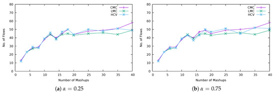
Figure 8.
Number of flows.
Note that, if mashups were outside the cloud, then more flows, between application components and the cloud in this case, would exist. The number of flows would be (see Figure 5). These values are not shown in order not to disturb the visualization of results from strategies. Flows would also have higher transfer delays, as these are not confined to internal transfers inside the cloud.
6. Conclusions
In this article, a resource allocation model for Se-aaS business models was addressed. The model fits multiple emerging IoT Se-aaS business models, including the ones where client applications have bindings to mashups in the cloud, each mashup combining one or more devices. This way, applications can share devices registered in the cloud, for their mashups to operate, using cloud and device resources more effectively. The advantage of managing mashups in the cloud, instead of managing them at the client side, is that delays associated with multiple traveling sessions of data to the client are avoided. A heuristic was also proposed, having the resource allocation model as a basis that allows for the implementation of strategies leading to an efficient allocation of resources. The strategy with the best performance is HCV because devices are used for the materialization of virtual Things with more mashup elements mapped to it, while fulfilling more mashup elements. HCV picks the cheapest materialization from mashup elements with highest cost variance, based on the assumption that their late selection could significantly increase the overall cost. However, mashup elements having high cost variance end up being the ones with more compatible requirements, leading to a higher level of aggregation. This strategy may, however, be improved in the future in order to place virtual Thing’s workspace more efficiently. The heuristic framework may also be improved for other clique subgraphs (rather than just the maximum) to be explored.
Author Contributions
Conceptualization, methodology, formal analysis, and writing: J.G. and N.C.; Software, validation: J.G. and L.R.; Investigation: J.G.; Supervision and funding acquisition: N.C.
Funding
This work was supported by FCT (Foundation for Science and Technology) from Portugal within CEOT (Center for Electronic, Optoelectronic and Telecommunications) and UID/MULTI/00631/2019 project.
Conflicts of Interest
The authors declare no conflict of interest.
References
- Fortino, G.; Russo, W.; Savaglio, C.; Viroli, M.; Zhou, M. Modeling Opportunistic IoT Services in Open IoT Ecosystems. In Proceedings of the 18th Workshop “From Objects to Agents”, Calabria, Italy, 15–16 June 2017. [Google Scholar]
- Guinard, D.; Trifa, V. Building the Web of Things; Manning Publications: Shelter Island, NY, USA, 2016. [Google Scholar]
- Perera, C.; Zaslavsky, A.; Christen, P.; Georgakopoulos, D. Sensing as a Service Model for Smart Cities Supported by Internet of Things. Trans. Emerg. Telecommun. Technol. 2014, 25, 81–93. [Google Scholar] [CrossRef]
- Kim, M.; Asthana, M.; Bhargava, S.; Iyyer, K.K.; Tangadpalliwar, R.; Gao, J. Developing an On-Demand Cloud-Based Sensing-as-a-Service System for Internet of Things. J. Comput. Netw. Commun. 2016, 2016, 3292783. [Google Scholar] [CrossRef]
- Duan, Y.; Fu, G.; Zhou, N.; Sun, X.; Narendra, N.C.; Hu, B. Everything as a Service(XaaS) on the Cloud: Origins, Current and Future Trends. In Proceedings of the IEEE 8th International Conference on Cloud Computing, New York, NY, USA, 7 June–2 July 2015. [Google Scholar]
- Misra, S.; Chatterjee, S.; Obaidat, M.S. On Theoretical Modeling of Sensor Cloud: A Paradigm Shift From Wireless Sensor Network. IEEE Syst. J. 2017, 11, 1084–1093. [Google Scholar] [CrossRef]
- Sheng, X.; Tang, J.; Xiao, X.; Xue, G. Sensing as a Service: Challenges, Solutions and Future Directions. IEEE Sens. J. 2013, 13, 3733–3741. [Google Scholar] [CrossRef]
- Pouryazdan, M.; Kantarci, B.; Soyata, T.; Foschini, L.; Song, H. Quantifying User Reputation Scores, Data Trustworthiness, and User Incentives in Mobile Crowd-Sensing. IEEE Access 2017, 5, 1382–1397. [Google Scholar] [CrossRef]
- Madria, S. Sensor Cloud: Sensing-as-Service Paradigm. In Proceedings of the IEEE International Conference on Mobile Data Management, Aalborg, Denmark, 25–28 June 2018. [Google Scholar]
- Al-Fagih, M.A.E.; Al-Turjman, F.M.; Alsalih, W.M.; Hassanein, H.S. Priced Public Sensing Framework for Heterogeneous IoT Architectures. IEEE Trans. Emerg. Top. Comput. 2013, 1, 133–147. [Google Scholar] [CrossRef]
- Petrolo, R.; Loscrì, V.; Mitton, N. Towards a Smart City Based on Cloud of Things, a Survey on the Smart City Vision and Paradigms. Trans. Emerg. Telecommun. Technol. 2017, 28, e2931. [Google Scholar] [CrossRef]
- Misra, S.; Bera, S.; Mondal, A.; Tirkey, R.; Chao, H.; Chattopadhyay, S. Optimal Gateway Selection in Sensor-Cloud Framework for Health Monitoring. IET Wirel. Sens. Syst. 2014, 4, 61–68. [Google Scholar] [CrossRef]
- Hsu, Y.-C.; Lin, C.-H.; Chen, W.-T. Design of a Sensing Service Architecture for Internet of Things with Semantic Sensor Selection. In Proceedings of the International Conference UTC-ATC-ScalCom, Bali, Indonesia, 9–12 December 2014. [Google Scholar]
- Lai, C.-C.; Chao, H.-C.; Lai, Y.; Wan, J. Cloud-Assisted Real-Time Transrating for HTTP Live Streaming. IEEE Wirel. Commun. 2013, 20, 62–70. [Google Scholar]
- Lai, C.-F.; Wang, H.; Chao, H.-C.; Nan, G. A Network and Device Aware QoS Approach for Cloud-Based Mobile Streaming. IEEE Trans. Multimed. 2013, 15, 747–757. [Google Scholar] [CrossRef]
- Wang, W.; Wang, Q.; Sohraby, K. Multimedia Sensing as a Service (MSaaS): Exploring Resource Saving Potentials of at Cloud-Edge IoTs and Fogs. IEEE Internet Things J. 2017, 4, 487–495. [Google Scholar] [CrossRef]
- Xu, Y.; Mao, S. A Survey of Mobile Cloud Computing for Rich Media Applications. IEEE Wirel. Commun. 2013, 20, 46–53. [Google Scholar] [CrossRef]
- Zhu, C.; Li, X.; Ji, H.; Leung, V.C.M. Towards Integration of Wireless Sensor Networks and Cloud Computing. In Proceedings of the International Conference CloudCom, Vancouver, BC, Canada, 30 November–3 December 2015. [Google Scholar]
- Kumar, L.P.D.; Grace, S.S.; Krishnan, A.; Manikandan, V.M.; Chinraj, R.; Sumalat, M.R. Data Filtering in Wireless Sensor Networks using Neural Networks for Storage in Cloud. In Proceedings of the International Conference ICRTIT, Chennai, Tamil Nadu, India, 19–21 April 2012. [Google Scholar]
- Zaslavsky, A.; Perera, C.; Georgakopoulos, D. Sensing as a Service and Big Data. In Proceedings of the International Conference on Advances in Cloud Computing, Bangalore, India, 4–6 July 2012. [Google Scholar]
- Distefano, S.; Merlino, G.; Puliafito, A. Sensing and Actuation as a Service: a New Development for Clouds. In Proceedings of the IEEE 11th International Symposium on Network Computing and Applications, Cambridge, MA, USA, 23–25 August 2012. [Google Scholar]
- Deshwal, A.; Kohli, S.; Chethan, K.P. Information as a Service based Architectural Solution for WSN. In Proceedings of the IEEE International Conference on Communications in China (ICCC ’12), Beijing, China, 15–17 August 2012. [Google Scholar]
- Dinh, T.; Kim, Y. An efficient Sensor-Cloud Interactive Model for On-Demand Latency Requirement Guarantee. In Proceedings of the IEEE International Conference on Communications (ICC), Paris, France, 21–25 May 2017. [Google Scholar]
- Distefano, S.; Merlino, G.; Puliafito, A. A Utility Paradigm for IoT: The Sensing Cloud. Pervasive Mob. Comput. 2015, 20, 127–144. [Google Scholar] [CrossRef]
- Fortino, G.; Savaglio, C.; Palau, C.E.; de PugaM, J.S.; Ganzha, A.; Paprzycki, M.; Montesinos, M.; Liotta, A.; Llop, M. Towards multi-layer interoperability of heterogeneous IoT platforms: The INTER-IoT approach. In Integration, Interconnection, and Interoperability of IoT Systems; Springer: Cham, Switzerland, 2018. [Google Scholar]
- Ishi, Y.; Kawakami, T.; Yoshihisa, T.; Teranishi, Y.; Nakauchi, K.; Nishinaga, N. Design and Implementation of Sensor Data Sharing Platform for Virtualized Wide Area Sensor Networks. In Proceedings of the International Conference on P2P, Parallel, Grid, Cloud and Internet Computing, Victoria, BC, Canada, 12–14 November 2012. [Google Scholar]
- Casadei, R.; Fortino, G.; Pianini, D.; Russo, W.; Savaglio, C.; Viroli, M. Modelling and simulation of Opportunistic IoT Services with Aggregate Computing. Future Gener. Comput. Syst. 2019, 91, 252–262. [Google Scholar] [CrossRef]
- Compton, M.; Barnaghi, P.; Bermudez, L.; García-Castro, R.; Corcho, O.; Cox, S.; Graybeal, J.; Hauswirth, M.; Henson, C.; Herzog, A.; et al. The SSN Ontology of the W3C Semantic Sensor Network Incubator Group. Web Semant. Sci. Serv. Agents World Wide Web 2012, 17, 25–32. [Google Scholar] [CrossRef]
- Blackstock, M.; Lea, R. IoT mashups with the WoTKit. In Proceedings of the IEEE International Conference on the Internet of Things (IOT), Wuxi, China, 24–26 October 2012. [Google Scholar]
- Barnaghi, P.; Wang, W.; Taylor, C.H.A.K. Semantics for the Internet of Things: Early progress and back to the future. Int. J. Semant. Web Inf. Syst. 2012, 8, 1–21. [Google Scholar] [CrossRef]
- Onat, F.A.; Stojmenovic, I. Generating Random Graphs for Wireless Actuator Networks. In Proceedings of the IEEE International Symposium on a World of Wireless, Mobile and Multimedia Networks, Espoo, Finland, 18–21 June 2007. [Google Scholar]
© 2019 by the authors. Licensee MDPI, Basel, Switzerland. This article is an open access article distributed under the terms and conditions of the Creative Commons Attribution (CC BY) license (http://creativecommons.org/licenses/by/4.0/).